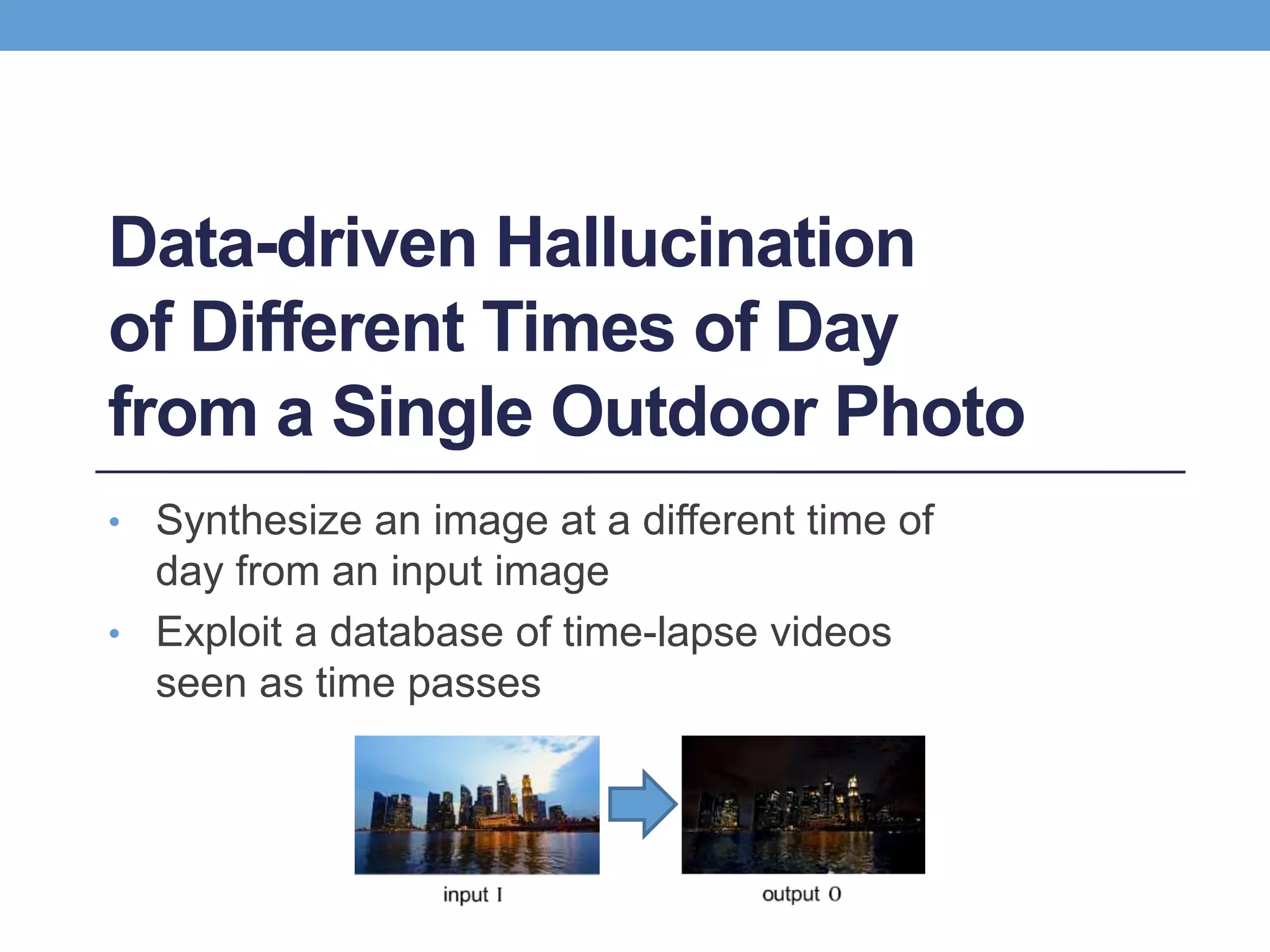
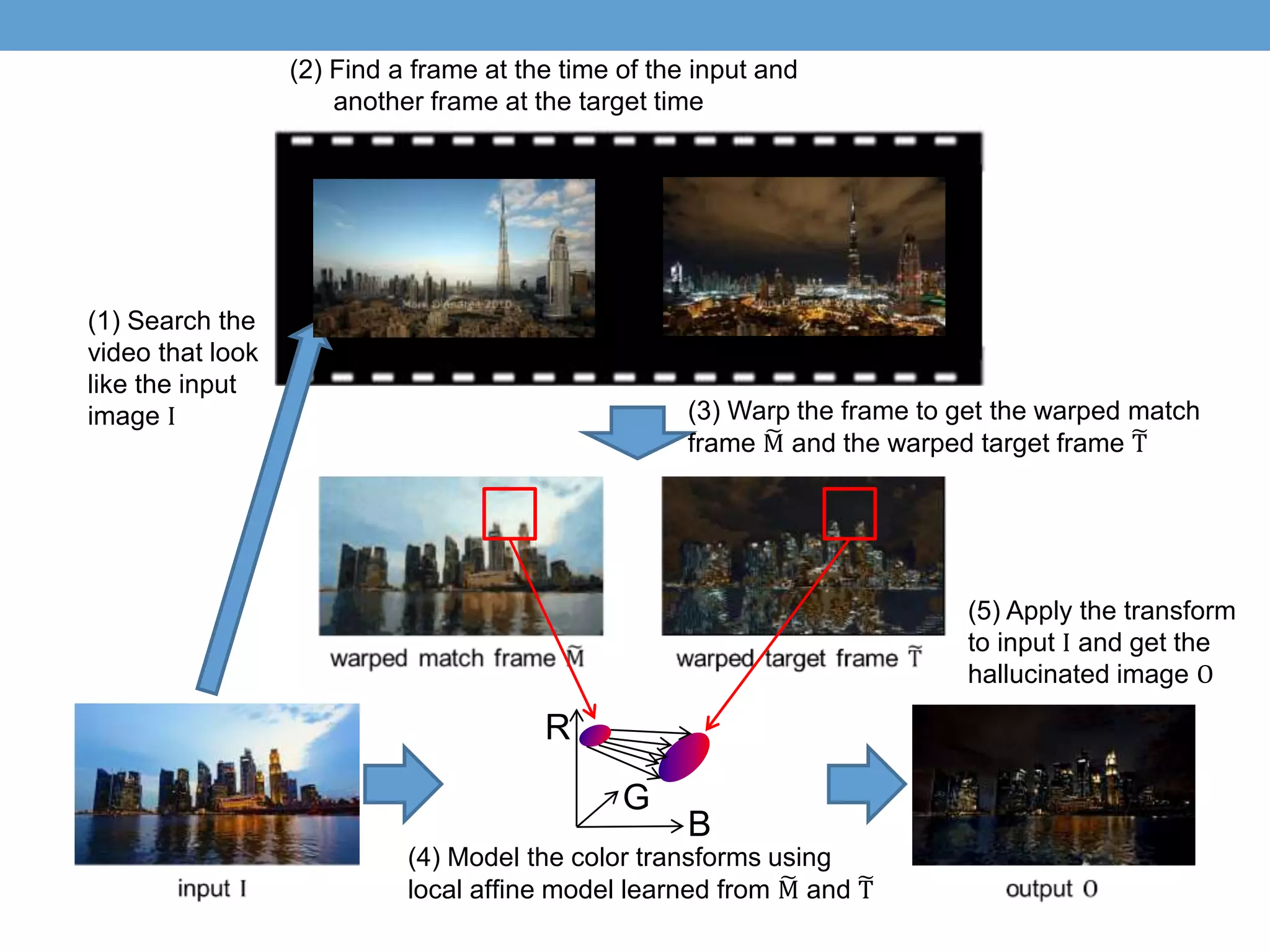
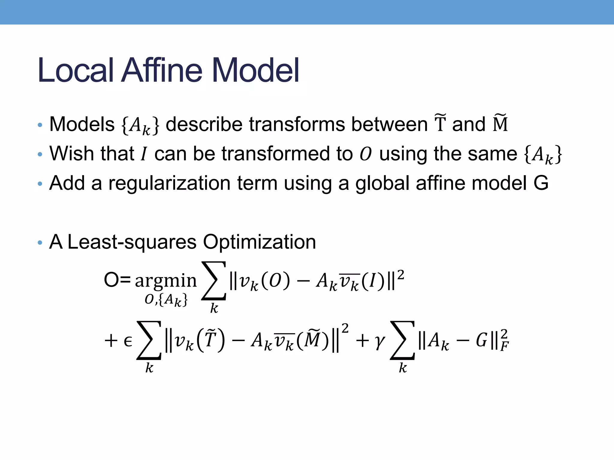
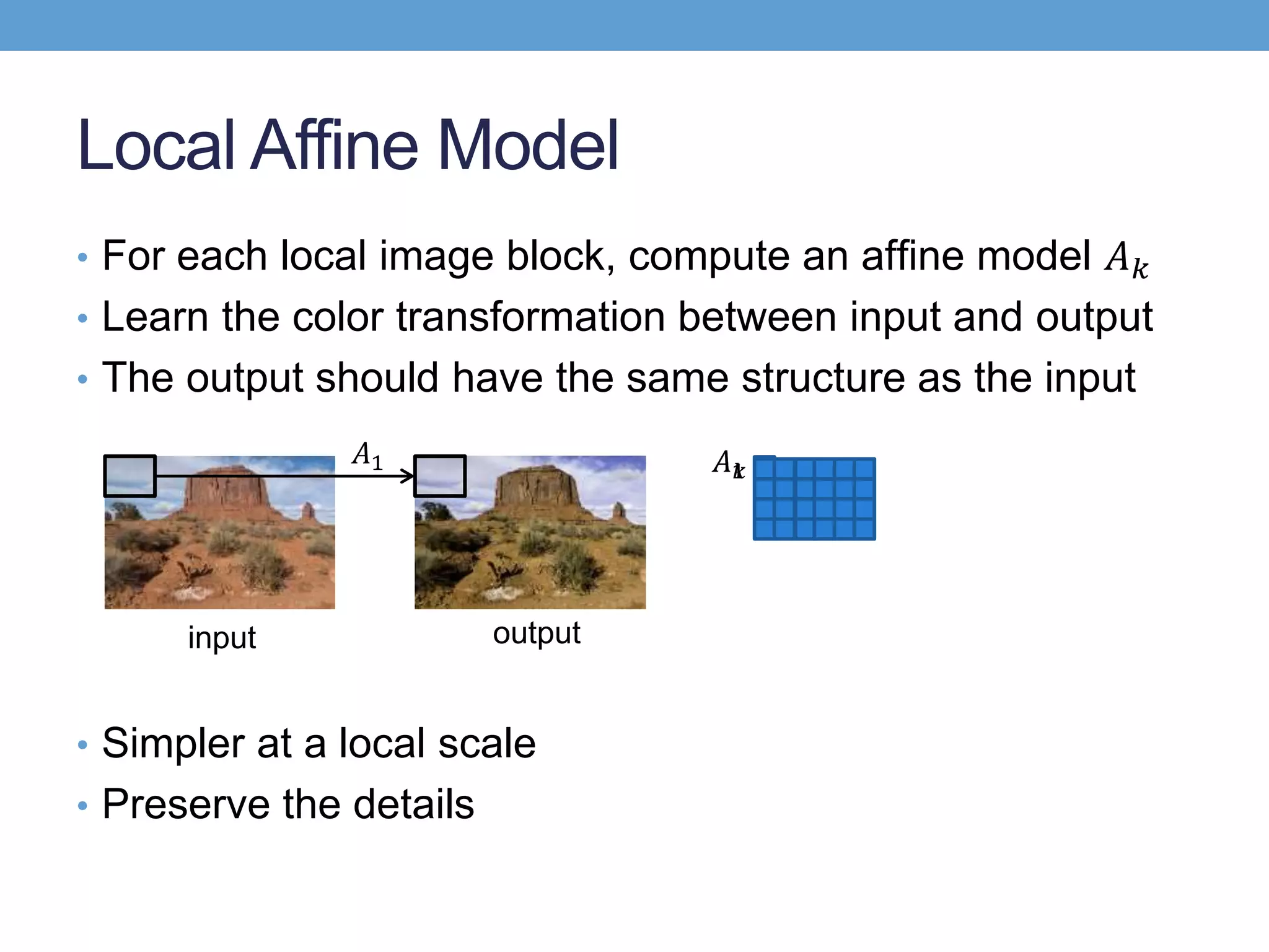
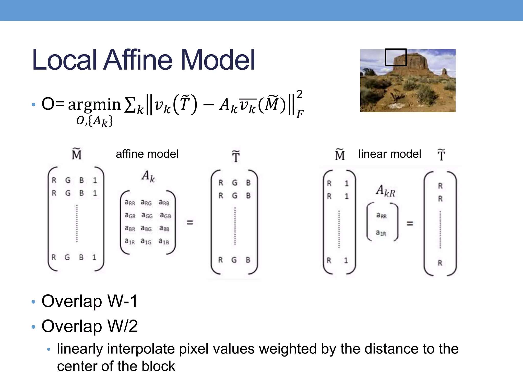
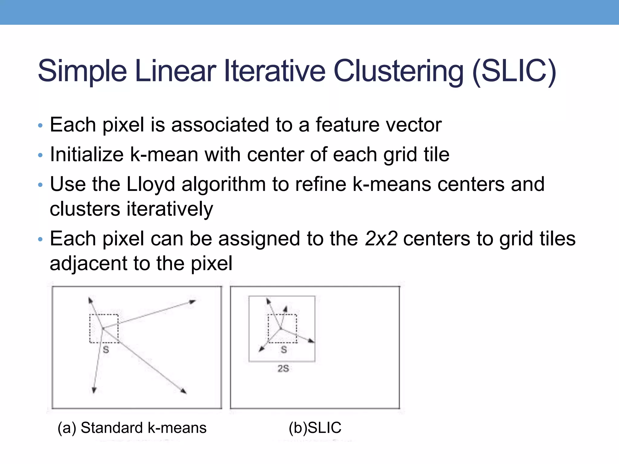
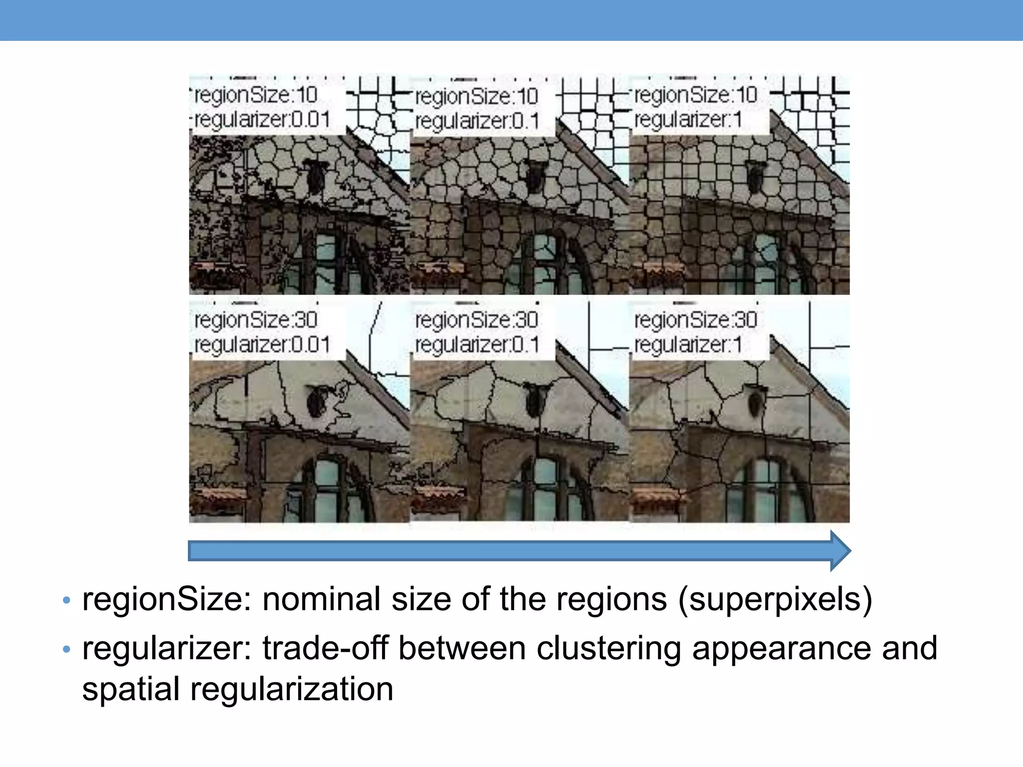
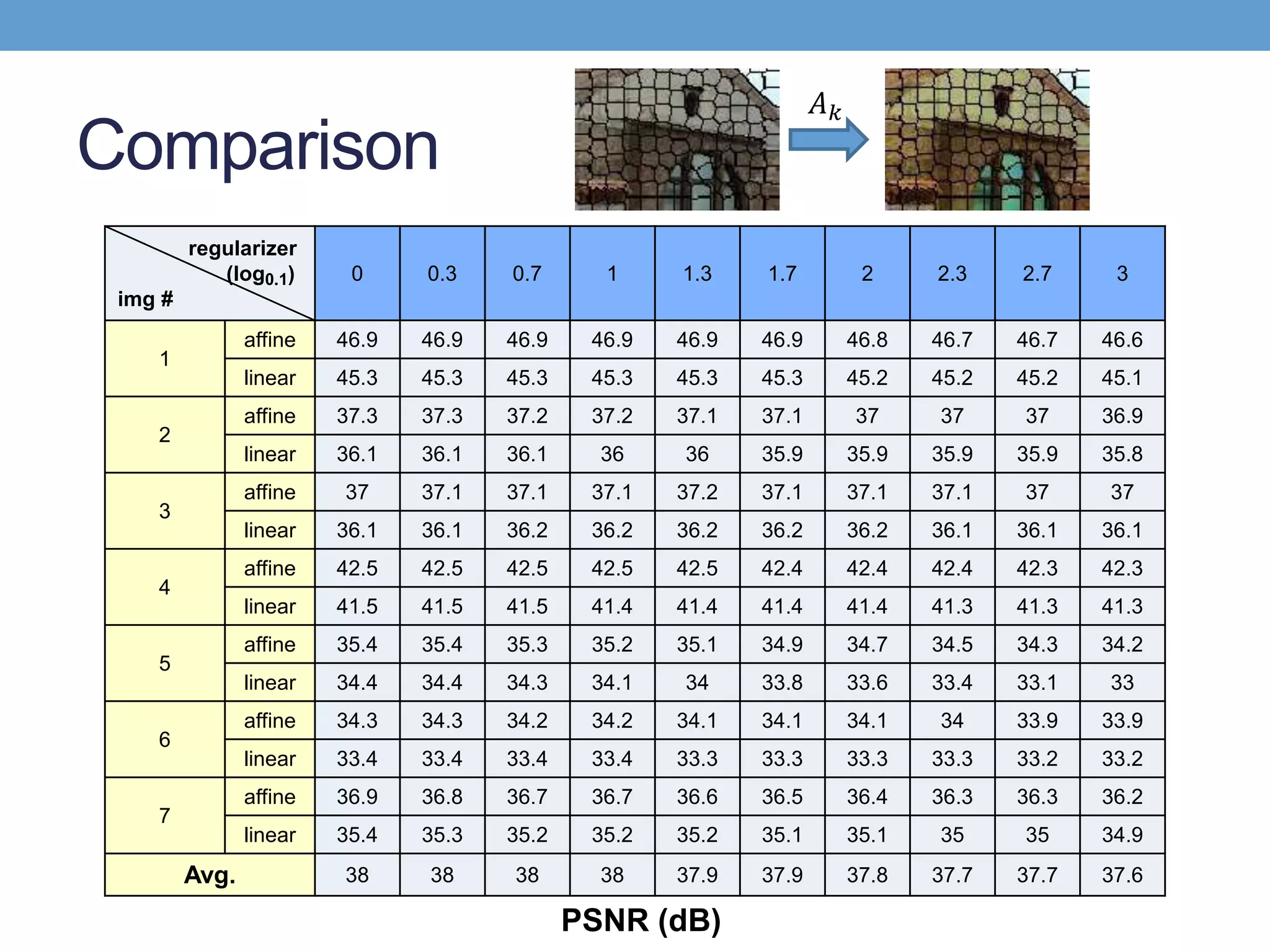
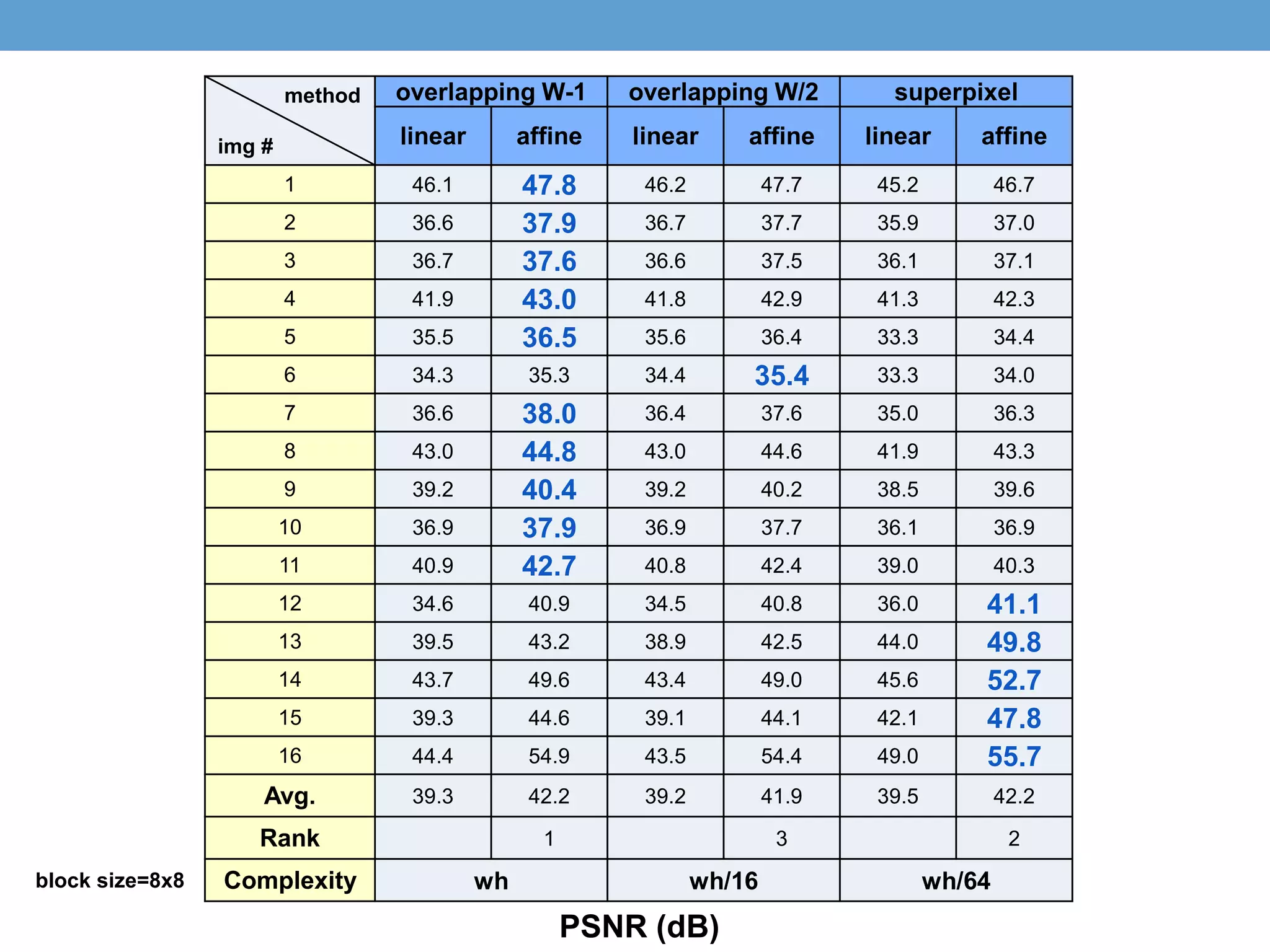
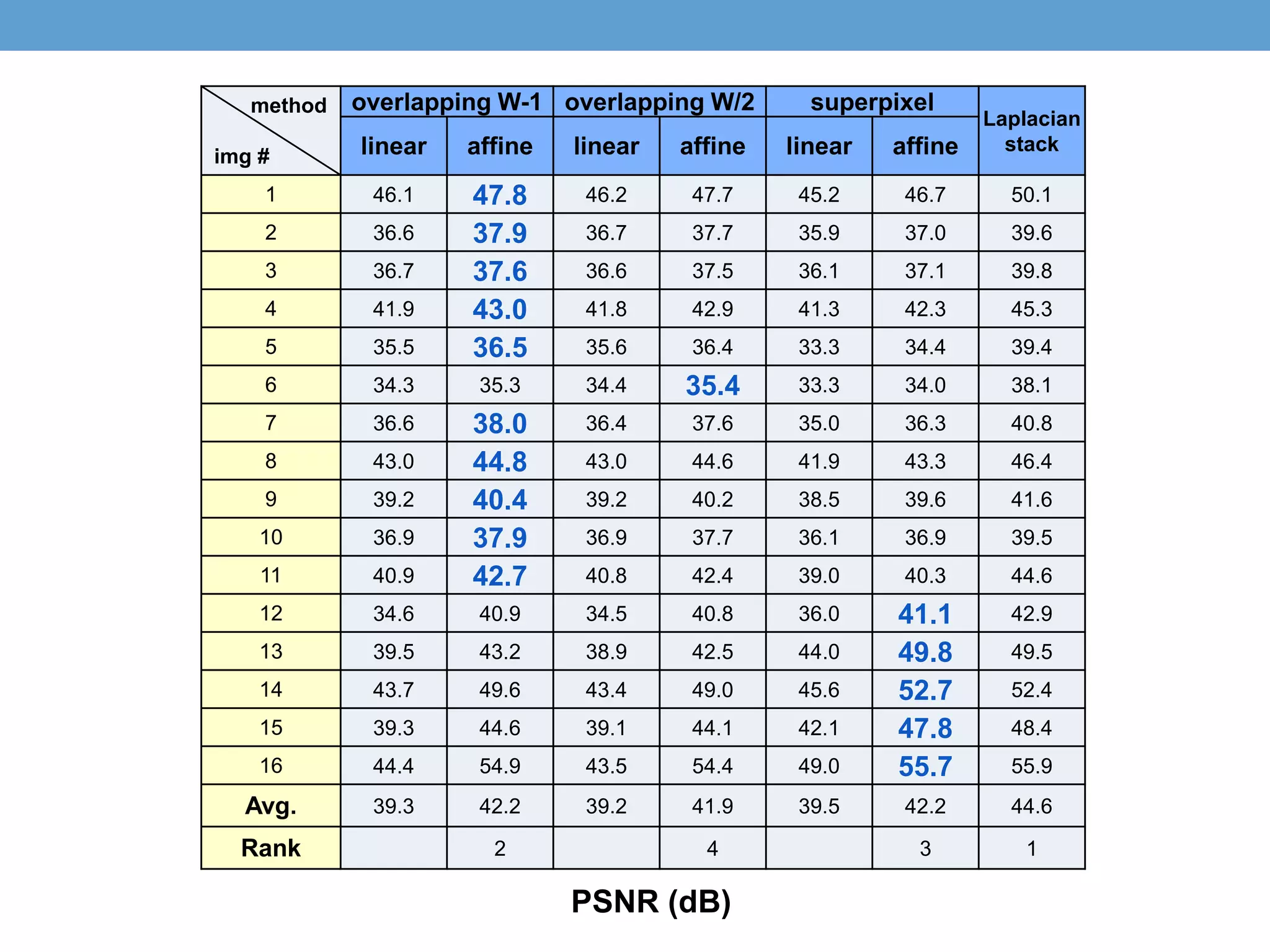
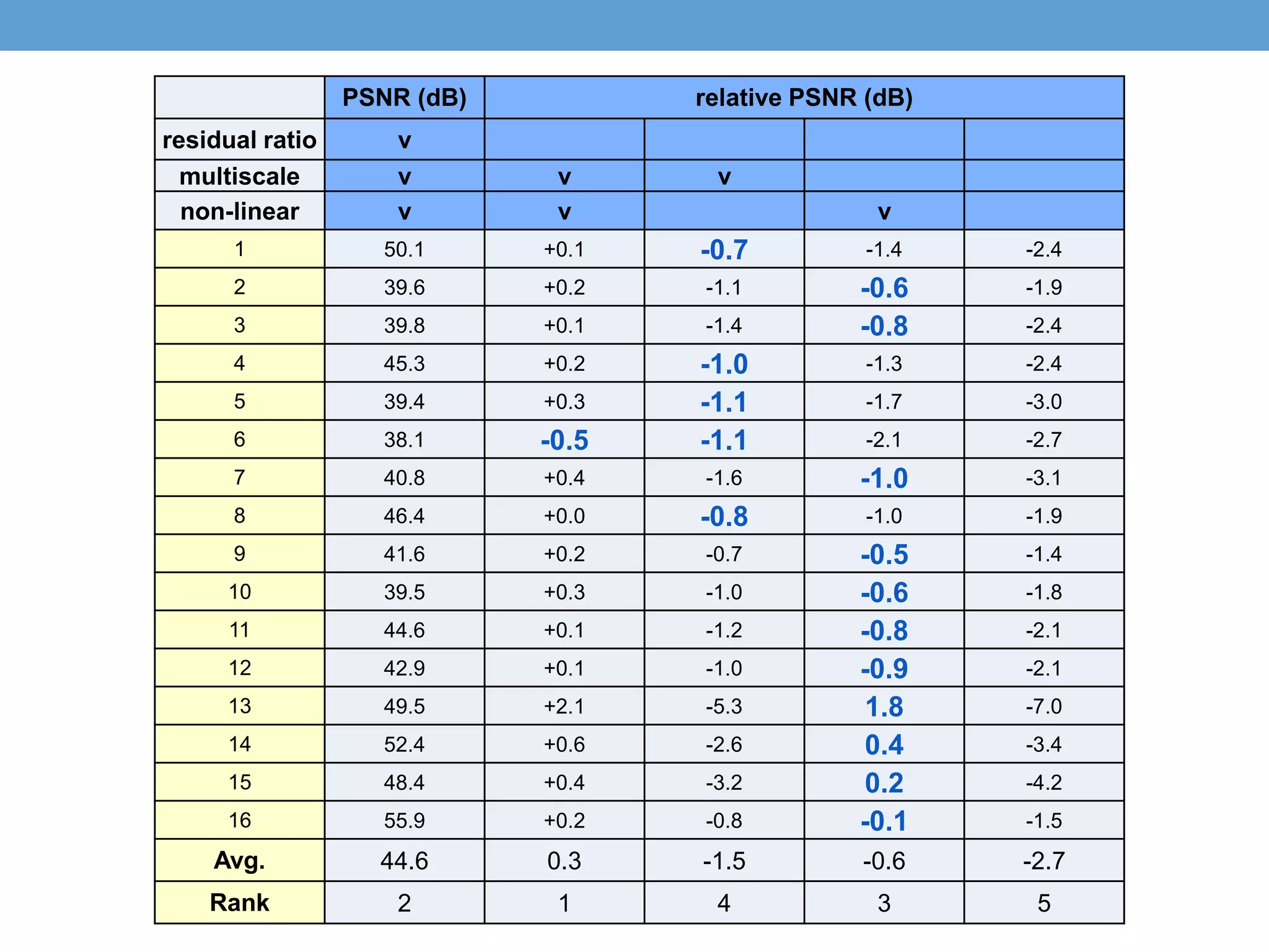
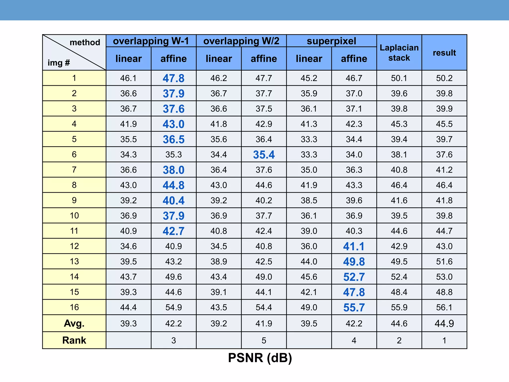
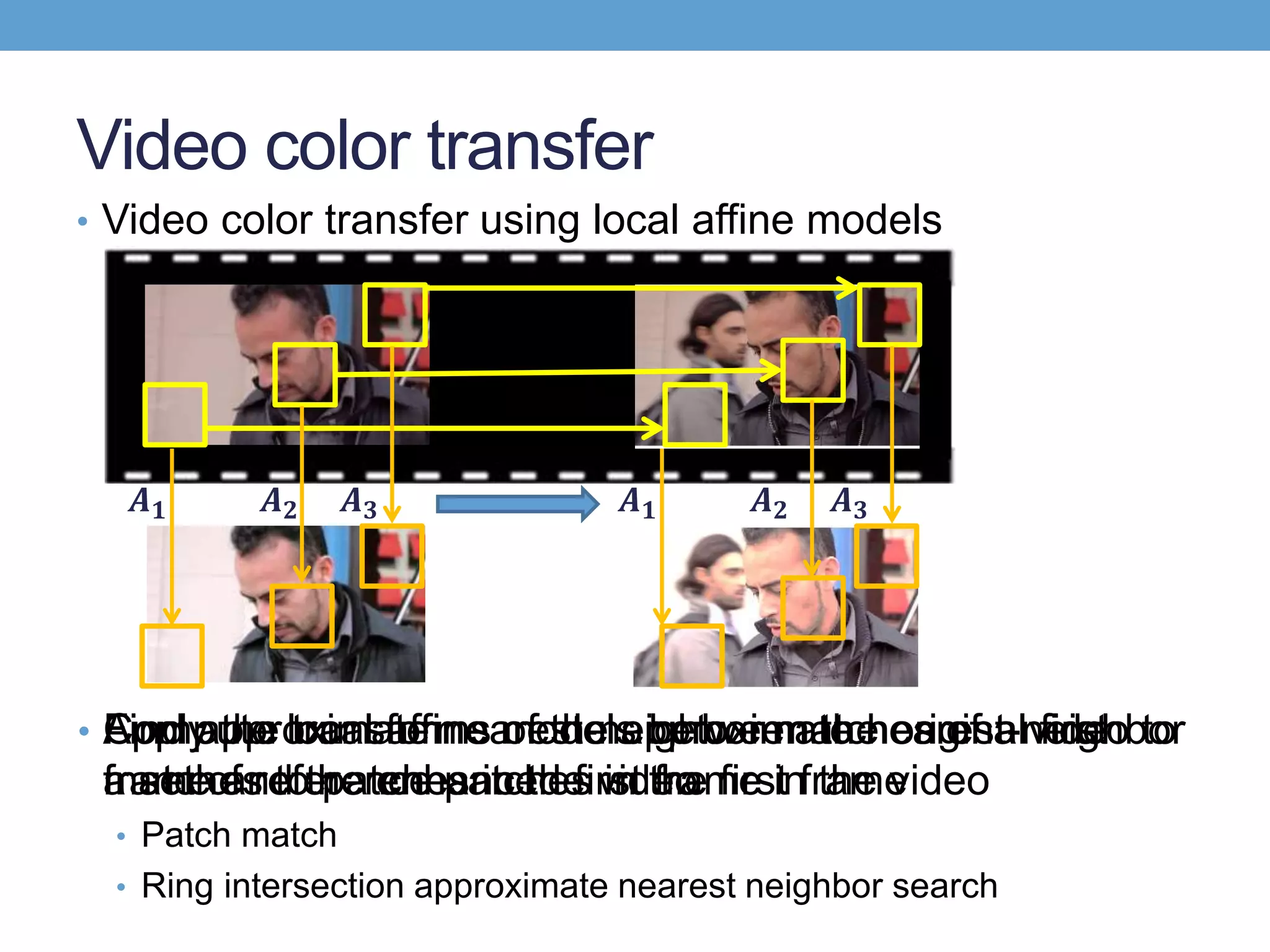
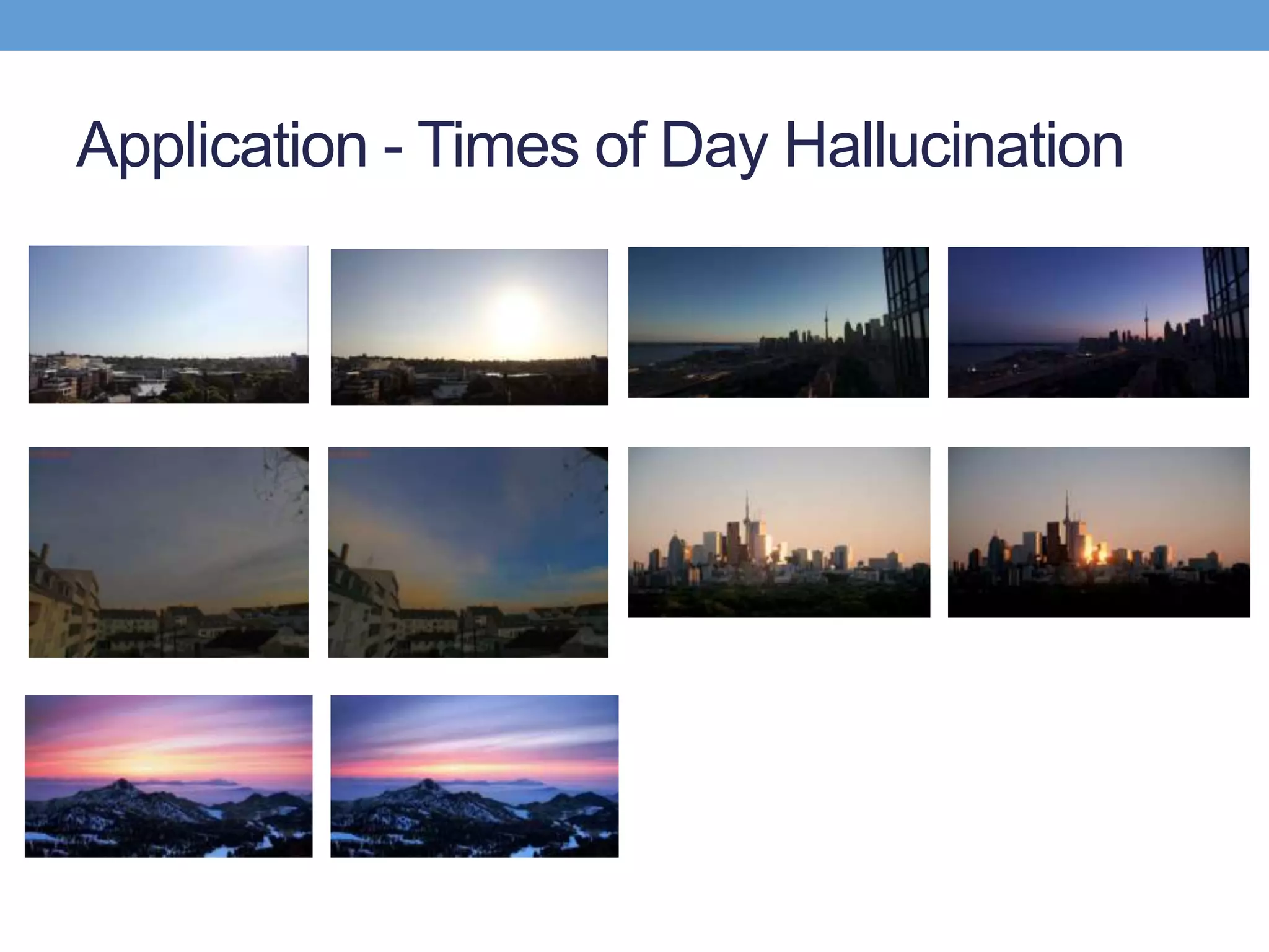
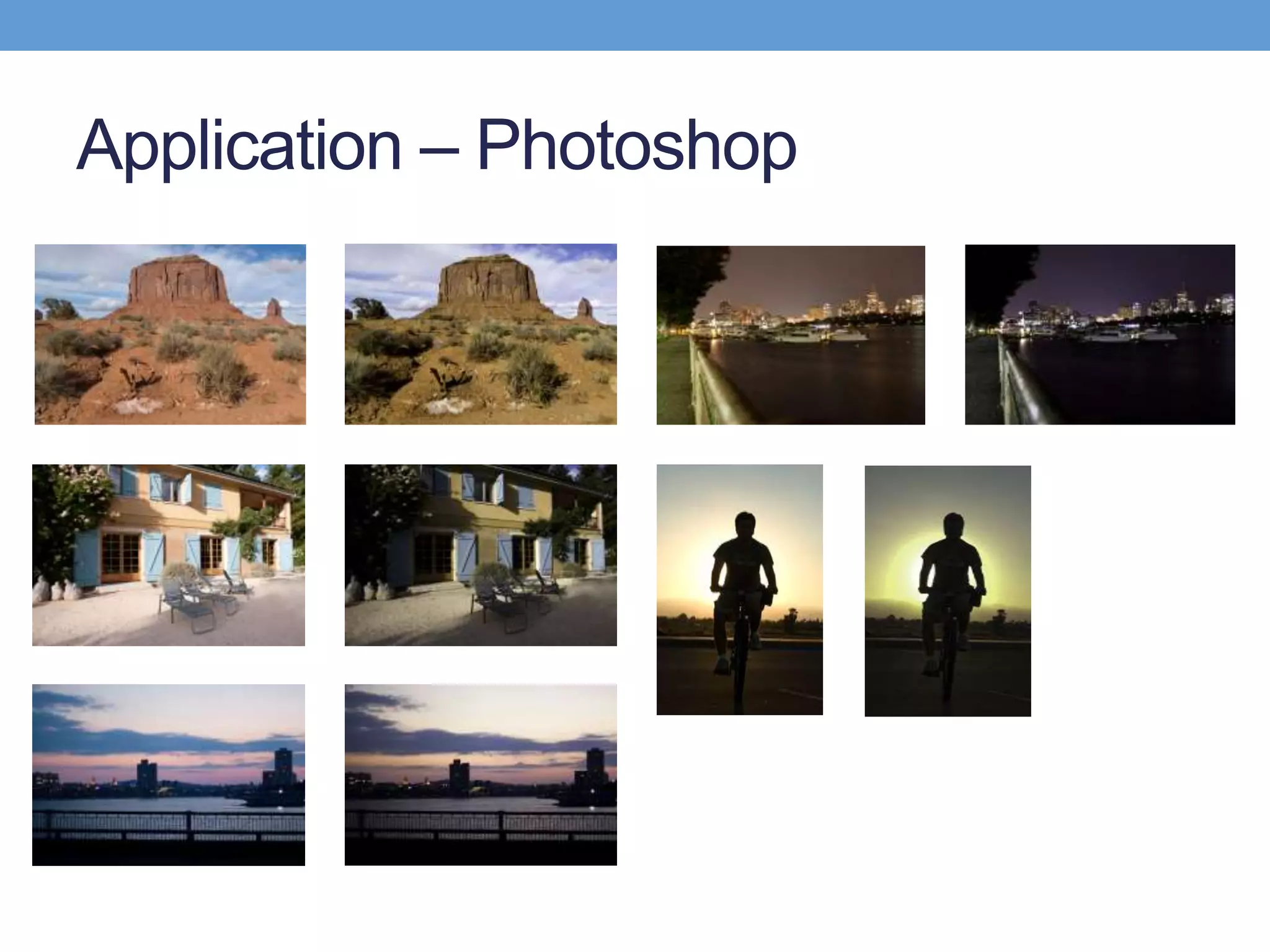
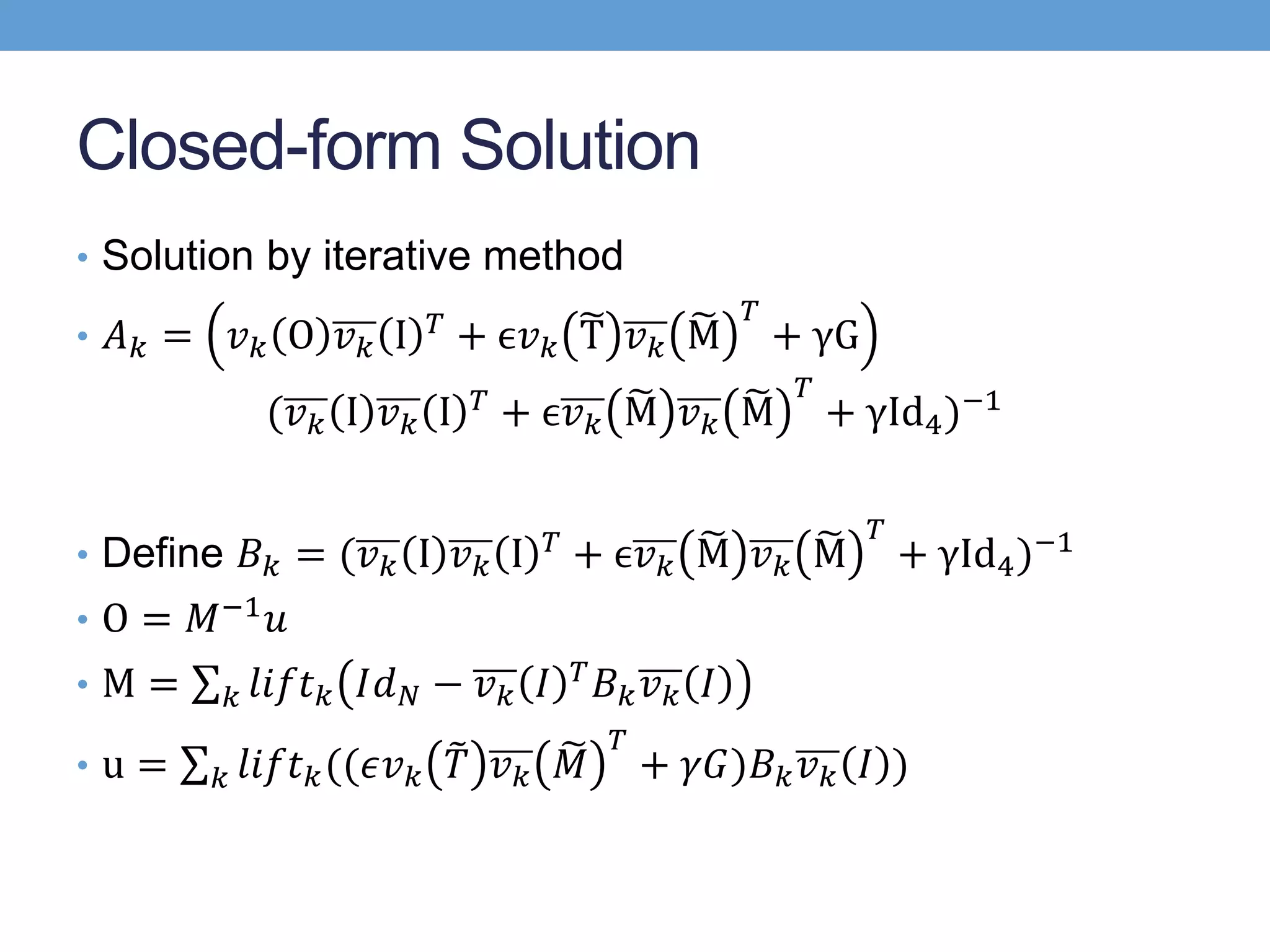
The document discusses several techniques for data-driven hallucination of different times of day from a single outdoor photo. It proposes using a local affine model to learn color transformations between frames from a matched video clip. The model is optimized using a least squares approach with regularization. It also discusses using superpixel segmentation and comparing performance of the local affine model versus a linear model.

1. Analysis of
Local Affine Model
電機三 黃馨平

2. Color Transfer
Times of day hallucination
Photoshop

3. Video Color Transfer
• Per-frame color transfer
• Computationally intensive
• Times of day hallucination for a 3-min video
• 180 sec x 25 frame/sec x 50 sec/frame = 5 hours
• Lack of temporal consistency
• Use local affine models

4. Data-driven Hallucination
of Different Times of Day
from a Single Outdoor Photo
• Synthesize an image at a different time of
day from an input image
• Exploit a database of time-lapse videos
seen as time passes

5. R
G
B
(1) Search the
video that look
like the input
image I
(2) Find a frame at the time of the input and
another frame at the target time
(3) Warp the frame to get the warped match
frame M and the warped target frame T
(4) Model the color transforms using
local affine model learned from M and T
(5) Apply the transform
to input I and get the
hallucinated image O

6. Local Affine Model
• Models {𝐴 𝑘} describe transforms between T and M
• Wish that 𝐼 can be transformed to 𝑂 using the same 𝐴 𝑘
• Add a regularization term using a global affine model G
• A Least-squares Optimization
Ο= argmin
𝑂,{𝐴 𝑘}
𝑘
𝑣 𝑘 𝑂 − 𝐴 𝑘 𝑣 𝑘(𝐼) 2
+ ϵ
𝑘
𝑣 𝑘 𝑇 − 𝐴 𝑘 𝑣 𝑘( 𝑀)
2
+ 𝛾
𝑘
𝐴 𝑘 − 𝐺 𝐹
2

7. • For each local image block, compute an affine model 𝐴 𝑘
• Learn the color transformation between input and output
• The output should have the same structure as the input
• Simpler at a local scale
• Preserve the details
Local Affine Model
input output
𝐴1 𝐴1𝐴 𝑘

8. Local Affine Model
• Ο= argmin
𝑂,{𝐴 𝑘}
𝑘 𝑣 𝑘 𝑇 − 𝐴 𝑘 𝑣 𝑘( 𝑀) 𝐹
2
affine model linear model
• Overlap W-1
• Overlap W/2
• linearly interpolate pixel values weighted by the distance to the
center of the block

9. SLIC Super-pixels
• Partition an image into multiple segments
• Pixels with the same label share certain
characteristics
• A spatially localized version of k-means
clustering

10. Simple Linear Iterative Clustering (SLIC)
• Each pixel is associated to a feature vector
• Initialize k-mean with center of each grid tile
• Use the Lloyd algorithm to refine k-means centers and
clusters iteratively
• Each pixel can be assigned to the 2x2 centers to grid tiles
adjacent to the pixel
(a) Standard k-means (b)SLIC

11. • regionSize: nominal size of the regions (superpixels)
• regularizer: trade-off between clustering appearance and
spatial regularization

12. Comparison
regularizer
(log0.1)
img #
0 0.3 0.7 1 1.3 1.7 2 2.3 2.7 3
1
affine 46.9 46.9 46.9 46.9 46.9 46.9 46.8 46.7 46.7 46.6
linear 45.3 45.3 45.3 45.3 45.3 45.3 45.2 45.2 45.2 45.1
2
affine 37.3 37.3 37.2 37.2 37.1 37.1 37 37 37 36.9
linear 36.1 36.1 36.1 36 36 35.9 35.9 35.9 35.9 35.8
3
affine 37 37.1 37.1 37.1 37.2 37.1 37.1 37.1 37 37
linear 36.1 36.1 36.2 36.2 36.2 36.2 36.2 36.1 36.1 36.1
4
affine 42.5 42.5 42.5 42.5 42.5 42.4 42.4 42.4 42.3 42.3
linear 41.5 41.5 41.5 41.4 41.4 41.4 41.4 41.3 41.3 41.3
5
affine 35.4 35.4 35.3 35.2 35.1 34.9 34.7 34.5 34.3 34.2
linear 34.4 34.4 34.3 34.1 34 33.8 33.6 33.4 33.1 33
6
affine 34.3 34.3 34.2 34.2 34.1 34.1 34.1 34 33.9 33.9
linear 33.4 33.4 33.4 33.4 33.3 33.3 33.3 33.3 33.2 33.2
7
affine 36.9 36.8 36.7 36.7 36.6 36.5 36.4 36.3 36.3 36.2
linear 35.4 35.3 35.2 35.2 35.2 35.1 35.1 35 35 34.9
Avg. 38 38 38 38 37.9 37.9 37.8 37.7 37.7 37.6
PSNR (dB)
𝐴 𝑘

13. method
img #
overlapping W-1 overlapping W/2 superpixel
linear affine linear affine linear affine
1 46.1 47.8 46.2 47.7 45.2 46.7
2 36.6 37.9 36.7 37.7 35.9 37.0
3 36.7 37.6 36.6 37.5 36.1 37.1
4 41.9 43.0 41.8 42.9 41.3 42.3
5 35.5 36.5 35.6 36.4 33.3 34.4
6 34.3 35.3 34.4 35.4 33.3 34.0
7 36.6 38.0 36.4 37.6 35.0 36.3
8 43.0 44.8 43.0 44.6 41.9 43.3
9 39.2 40.4 39.2 40.2 38.5 39.6
10 36.9 37.9 36.9 37.7 36.1 36.9
11 40.9 42.7 40.8 42.4 39.0 40.3
12 34.6 40.9 34.5 40.8 36.0 41.1
13 39.5 43.2 38.9 42.5 44.0 49.8
14 43.7 49.6 43.4 49.0 45.6 52.7
15 39.3 44.6 39.1 44.1 42.1 47.8
16 44.4 54.9 43.5 54.4 49.0 55.7
Avg. 39.3 42.2 39.2 41.9 39.5 42.2
Rank 1 3 2
Complexity wh wh/16 wh/64
PSNR (dB)
block size=8x8

14. Transform Recipes for Efficient
Cloud Photo Enhancement
• Limited computing power and battery life of
mobile devices
• Cloud image processing applications which
preserve the overall content of an image
• Use least time and energy cost of
uploading and downloading

15. (1) Generate a compressed input I of the input image I(2) Upload this image I along with the histogram of I(3) Upsample I and applies histogram transfer to compute a proxy input 𝐼(4) Generate a proxy output 𝑂 = f( 𝐼)(5) Compute a compact recipe r using 𝐼 and 𝑂，r 𝐼 ≈ 𝑓( 𝐼)(6) Download the recipe(7) Apply it on the original input I
• Process input I with a filter f to produce output O = f(I)
• Each recipe is specific to a given input-filter pair

16. Image Decomposition
• Multi-scale decomposition
• Work in {𝑌, 𝐶 𝑏, 𝐶𝑟} color space
• Coarsely model the chrominance transformation and
sophisticatedly model the luminance transformation
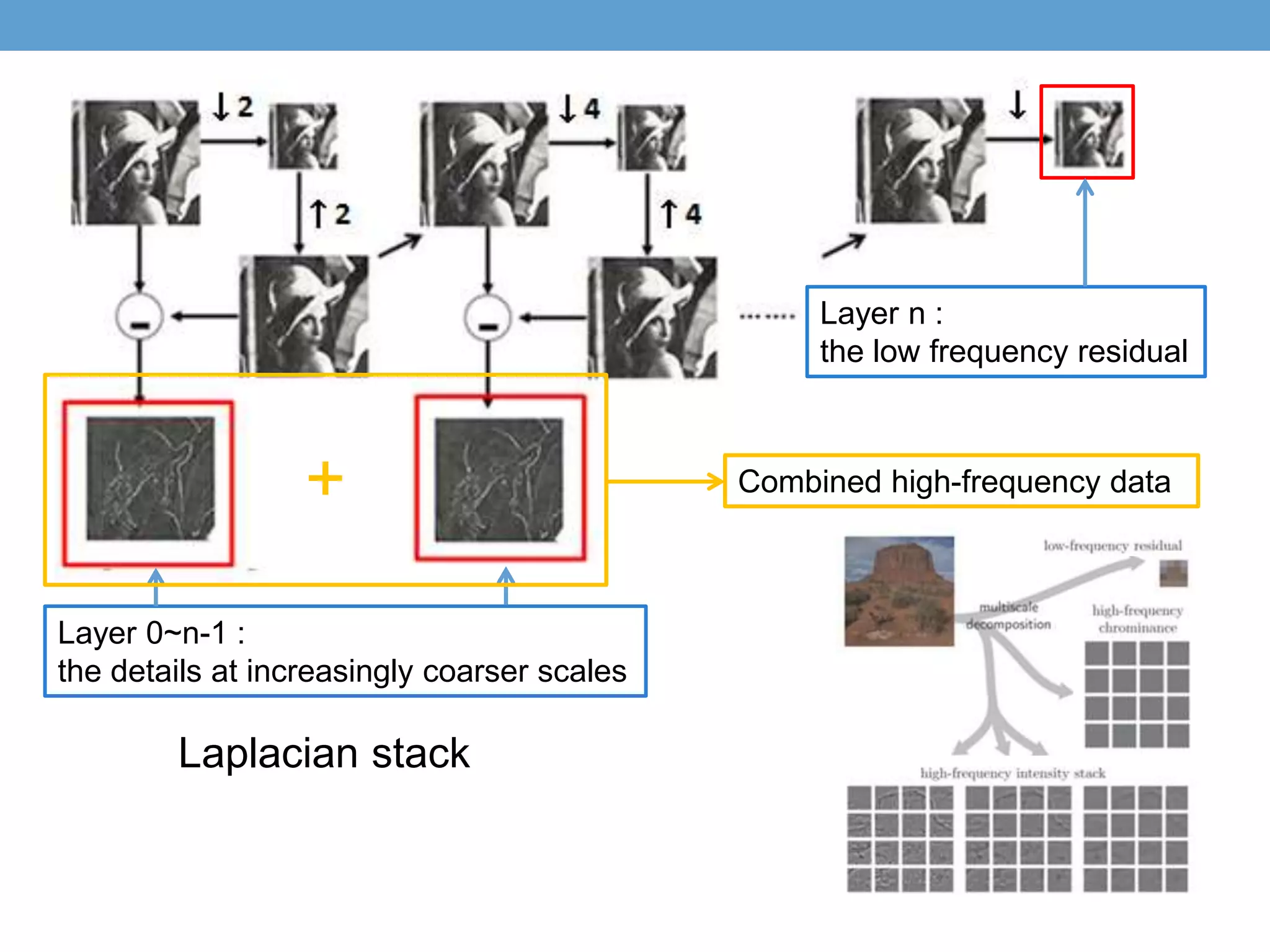
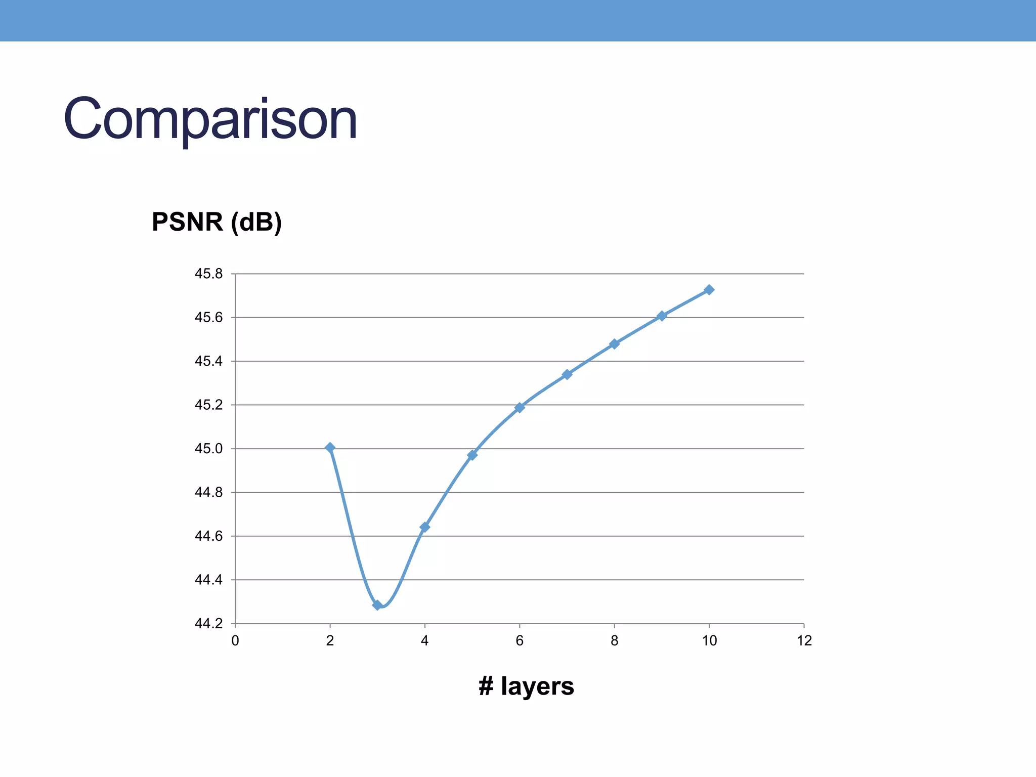
• Split 𝐼 and 𝑂 into n + 1 levels 𝐿[𝐼] and 𝐿[𝑂]
• First n levels represent the details at increasingly coarser scales
• Last level is the low frequency residual which affects a large area
and affect significantly in final reconstruction
• Combined high-frequency data
H I = 𝑙=0
𝑛−1
𝐿𝑙[𝐼]

17. Layer n :
the low frequency residual
Layer 0~n-1 :
the details at increasingly coarser scales
Combined high-frequency data+
Laplacian stack

18. Compute Recipes (1)
• The low frequency residual part of the transformation
𝑅 𝑐 𝑝 =
𝐿 𝑛 𝑂𝑐 𝑝 + 1
𝐿 𝑛 𝐼𝑐 𝑝 + 1
• Chrominance Transformations
𝑝𝜖ℬ
𝐻 𝑂𝑐𝑐 𝑝 − 𝐴 𝑐 ℬ 𝐻 𝐼 𝑝 − 𝑏 𝑐(ℬ) 2
affine function

19. Compute Recipes (2)
• Luminance Transformations
• Affine function - brightness and contrast
• Multiplicative factor to each stack level - multiscale effects
• Multiplicative factor to non-linearity terms
• Segment Function
• 𝑦𝑖 = min
ℬ
𝐻 𝐼 𝑌 +
𝑖
𝑘
(max
ℬ
𝐻 𝐼 𝑌 − min
ℬ
𝐻 𝐼 𝑌 ) , 𝑖 ∈ {1, … , 𝑘 − 1}
• 𝑠𝑖 ∙ = max ∙ −𝑦𝑖 , 0

20. Compute Recipes (3)
• 𝑝𝜖ℬ 𝐻 𝑂 𝑌 𝑝 − 𝐴 𝑌 ℬ 𝐻 𝐼 𝑝 − 𝑏 𝑌 ℬ − 𝑙=0
𝑛−1
𝑚𝑙 ℬ 𝐿𝑙 𝐼 𝑌 𝑝 − 𝑖=1
𝑘−1
𝑞𝑖(ℬ)𝑠𝑖(𝐻[𝐼 𝑌](𝑝))
2
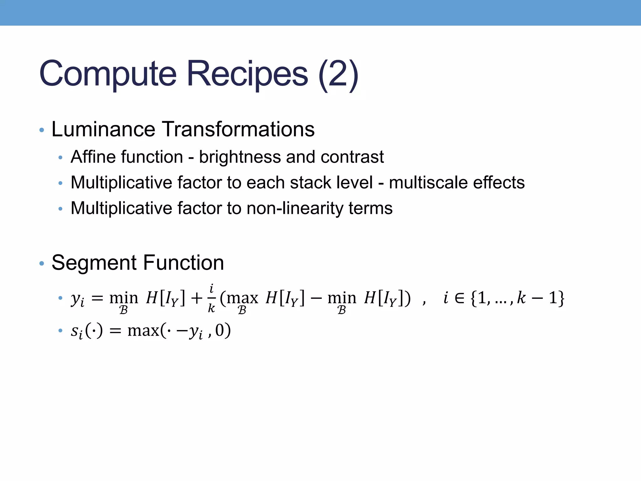
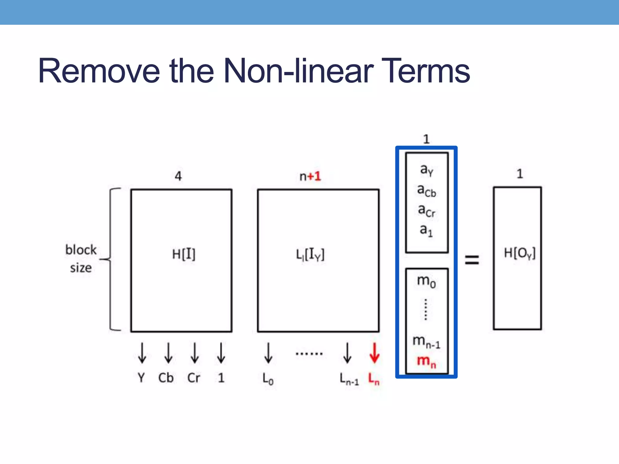
affine function multiplicative factor
to each stack level
multiplicative factor
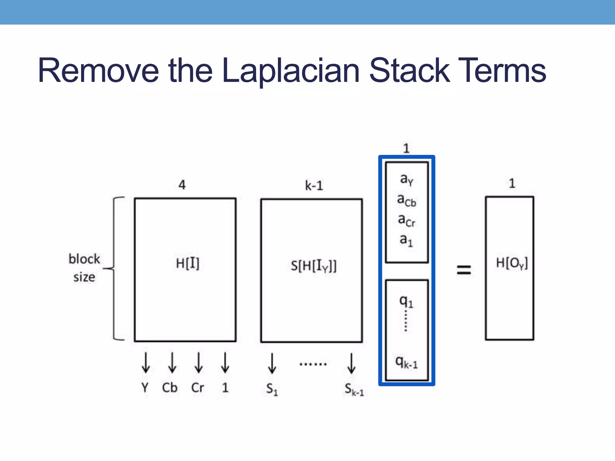
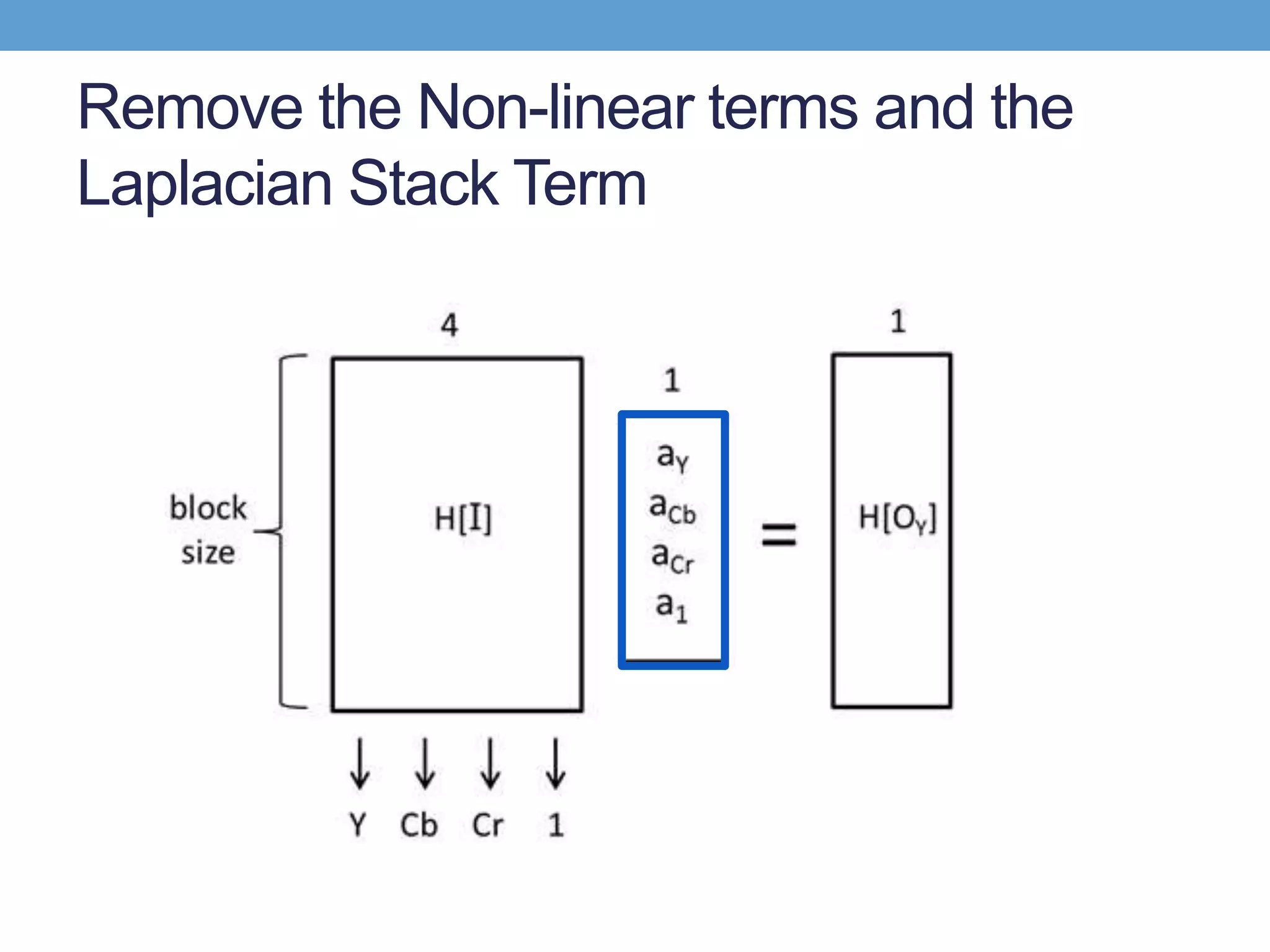
to non-linearity terms

21. Lasso Regression
• Include a penalty term to constrain the size of the
coefficients
• min
𝛽0,𝛽
(
1
2𝑁 𝑖=1
𝑁
(𝑦𝑖 − 𝛽0 − 𝑥𝑖
𝑇
𝛽)2+𝜆𝑃𝛼(𝛽))
• 𝑃𝛼 𝛽 =
1−𝛼
2
𝛽 2
2
+ 𝛼 𝛽 1 = 𝑗=1
𝑝
(
1−𝛼
2
𝛽𝑗
2
+ 𝛼 𝛽𝑗 )
• The penalty term Pα(β) interpolates between the L1 norm
of β and the squared L2 norm of β
• As λ increases, the number of nonzero components
of β decreases

22. Reconstructing
• Perform the same decomposition
• Apply the corresponding recipe coefficients to each term
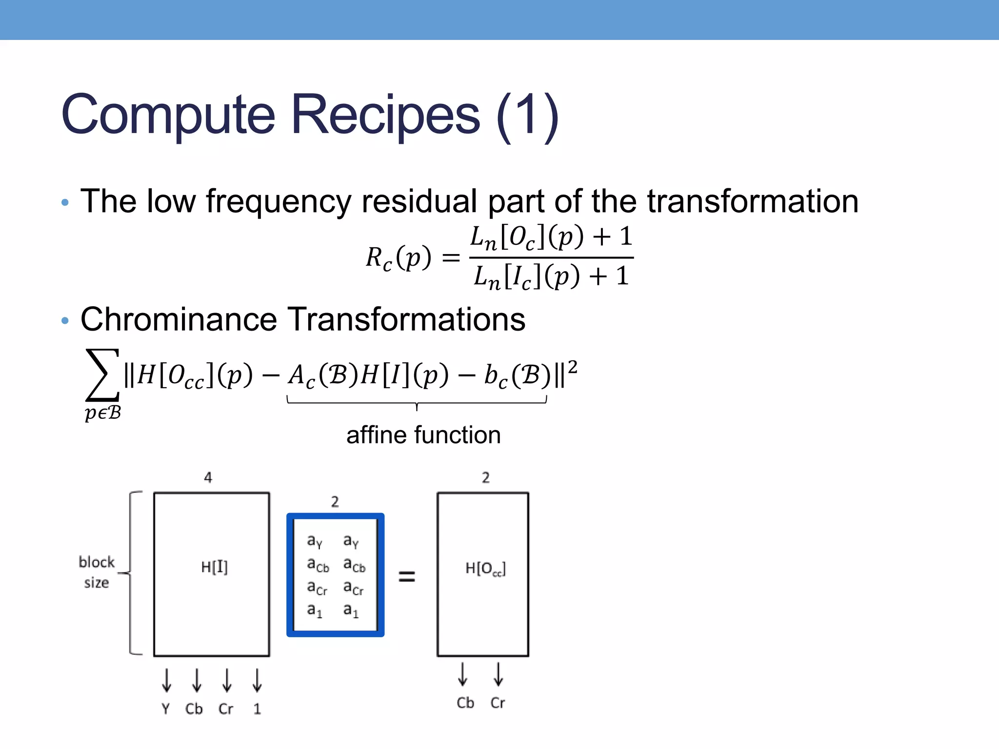
• L 𝑛 𝑂𝑐 𝑝 = 𝑅 𝑐 𝑝 𝐿 𝑛[𝐼𝑐](𝑝) + 1 − 1
• 𝐻ℬ O 𝑐𝑐 p = 𝐴 𝑐 ℬ 𝐻 𝐼 𝑝 + 𝑏 𝑐(ℬ)
• 𝐻ℬ O 𝑌 p = 𝐴 𝑌 ℬ 𝐻 𝐼 𝑝 + 𝑏 𝑌 ℬ +
𝑙=0
𝑛−1
𝑚𝑙 ℬ 𝐿𝑙 𝐼 𝑌 𝑝 + 𝑖=1
𝑘−1
𝑞𝑖(ℬ)𝑠𝑖(𝐻[𝐼 𝑌](𝑝))
• O = up L 𝑛 + H O 𝑐𝑐 + H[O 𝑌]
• Up-sample the low residual term
• Linearly interpolate other terms

23. # segments
img #
2 4 6 8 10 12 14 16 18 20
1 49.5 49.7 49.9 50.0 50.1 50.2 50.3 50.4 50.5 50.6
2 38.6 39.0 39.2 39.4 39.6 39.8 40.0 40.1 40.3 40.4
3 38.7 39.1 39.4 39.6 39.8 40.1 40.3 40.5 40.7 40.8
4 44.4 44.7 44.9 45.1 45.3 45.4 45.6 45.8 46.0 46.1
5 38.2 38.6 38.9 39.1 39.4 39.6 39.8 40.0 40.2 40.4
6 37.3 37.6 37.8 37.9 38.1 38.2 38.4 38.5 38.6 38.7
7 39.4 39.9 40.2 40.5 40.8 41.0 41.3 41.5 41.7 42.0
8 45.8 46.0 46.2 46.3 46.4 46.5 46.7 46.7 46.8 46.9
9 41.0 41.2 41.4 41.5 41.6 41.7 41.8 42.0 42.0 42.1
10 38.5 38.8 39.1 39.3 39.5 39.7 39.9 40.1 40.3 40.4
11 43.7 44.0 44.3 44.4 44.6 44.7 44.9 45.0 45.1 45.2
12 42.4 42.7 42.7 42.8 42.9 43.0 43.0 43.1 43.2 43.2
13 47.5 49.0 49.3 49.4 49.5 49.7 49.7 49.8 49.9 50.0
14 51.7 52.2 52.3 52.4 52.4 52.5 52.5 52.6 52.6 52.7
15 47.0 48.0 48.2 48.3 48.4 48.4 48.5 48.6 48.6 48.7
16 55.4 55.6 55.7 55.8 55.9 55.9 56.0 56.0 56.0 56.1
Avg. 43.7 44.1 44.3 44.5 44.6 44.8 44.9 45.0 45.2 45.3
PSNR (dB)

24. Comparison
43.6
43.8
44.0
44.2
44.4
44.6
44.8
45.0
45.2
45.4
0 5 10 15 20 25
# segments
PSNR (dB)

25. # layers
img #
2 3 4 5 6 7 8 9 10
1 51.1 50.0 50.1 50.3 50.5 50.7 50.8 50.9 51.0
2 40.1 39.4 39.6 39.8 40.0 40.2 40.3 40.5 40.6
3 40.1 39.6 39.8 40.0 40.2 40.4 40.5 40.7 40.9
4 45.7 45.0 45.3 45.5 45.7 45.9 46.2 46.4 46.5
5 39.9 39.1 39.4 39.8 40.1 40.5 40.7 41.0 41.3
6 39.2 37.9 38.1 38.5 38.7 38.7 38.9 39.1 39.3
7 41.5 40.4 40.8 41.2 41.6 41.9 42.1 42.4 42.7
8 48.1 46.4 46.4 46.6 46.7 46.9 47.0 47.1 47.1
9 42.5 41.5 41.6 41.8 41.9 42.0 42.1 42.2 42.3
10 40.3 39.4 39.5 39.8 40.0 40.3 40.5 40.7 40.9
11 46.0 44.6 44.6 44.8 45.0 45.2 45.4 45.5 45.6
12 42.9 42.8 42.9 43.0 43.0 43.1 43.1 43.2 43.2
13 47.0 47.5 49.5 50.9 51.5 51.7 51.8 51.8 51.9
14 51.6 51.4 52.4 52.8 53.0 53.1 53.1 53.1 53.2
15 47.7 47.6 48.4 48.7 48.8 48.9 48.9 49.0 49.0
16 56.4 55.8 55.9 56.0 56.1 56.2 56.2 56.3 56.3
Avg. 45.0 44.3 44.6 45.0 45.2 45.3 45.5 45.6 45.7
PSNR (dB)

26. Comparison
# layers
PSNR (dB)
44.2
44.4
44.6
44.8
45.0
45.2
45.4
45.6
45.8
0 2 4 6 8 10 12

27. method
img #
overlapping W-1 overlapping W/2 superpixel
Laplacian
stacklinear affine linear affine linear affine
1 46.1 47.8 46.2 47.7 45.2 46.7 50.1
2 36.6 37.9 36.7 37.7 35.9 37.0 39.6
3 36.7 37.6 36.6 37.5 36.1 37.1 39.8
4 41.9 43.0 41.8 42.9 41.3 42.3 45.3
5 35.5 36.5 35.6 36.4 33.3 34.4 39.4
6 34.3 35.3 34.4 35.4 33.3 34.0 38.1
7 36.6 38.0 36.4 37.6 35.0 36.3 40.8
8 43.0 44.8 43.0 44.6 41.9 43.3 46.4
9 39.2 40.4 39.2 40.2 38.5 39.6 41.6
10 36.9 37.9 36.9 37.7 36.1 36.9 39.5
11 40.9 42.7 40.8 42.4 39.0 40.3 44.6
12 34.6 40.9 34.5 40.8 36.0 41.1 42.9
13 39.5 43.2 38.9 42.5 44.0 49.8 49.5
14 43.7 49.6 43.4 49.0 45.6 52.7 52.4
15 39.3 44.6 39.1 44.1 42.1 47.8 48.4
16 44.4 54.9 43.5 54.4 49.0 55.7 55.9
Avg. 39.3 42.2 39.2 41.9 39.5 42.2 44.6
Rank 2 4 3 1
PSNR (dB)

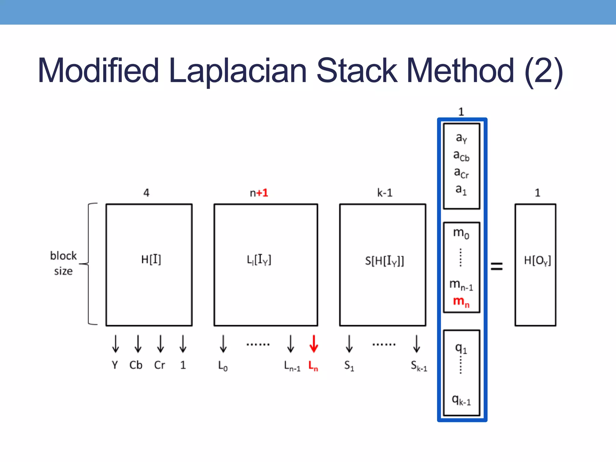
28. • H I = 𝑙=0
𝑛
𝐿𝑙[𝐼]
• Remove the low frequency residual
• Add a layer in laplacian stack and the high frequency term
Modified Laplacian Stack Method (1)
Layer 0~n-1
Layer n
Combined high-frequency data+

29. Modified Laplacian Stack Method (2)

30. Remove the Non-linear Terms

31. Remove the Laplacian Stack Terms

32. Remove the Non-linear terms and the
Laplacian Stack Term

33. PSNR (dB) relative PSNR (dB)
residual ratio v
multiscale v v v
non-linear v v v
1 50.1 +0.1 -0.7 -1.4 -2.4
2 39.6 +0.2 -1.1 -0.6 -1.9
3 39.8 +0.1 -1.4 -0.8 -2.4
4 45.3 +0.2 -1.0 -1.3 -2.4
5 39.4 +0.3 -1.1 -1.7 -3.0
6 38.1 -0.5 -1.1 -2.1 -2.7
7 40.8 +0.4 -1.6 -1.0 -3.1
8 46.4 +0.0 -0.8 -1.0 -1.9
9 41.6 +0.2 -0.7 -0.5 -1.4
10 39.5 +0.3 -1.0 -0.6 -1.8
11 44.6 +0.1 -1.2 -0.8 -2.1
12 42.9 +0.1 -1.0 -0.9 -2.1
13 49.5 +2.1 -5.3 1.8 -7.0
14 52.4 +0.6 -2.6 0.4 -3.4
15 48.4 +0.4 -3.2 0.2 -4.2
16 55.9 +0.2 -0.8 -0.1 -1.5
Avg. 44.6 0.3 -1.5 -0.6 -2.7
Rank 2 1 4 3 5

34. method
img #
overlapping W-1 overlapping W/2 superpixel
Laplacian
stack
result
linear affine linear affine linear affine
1 46.1 47.8 46.2 47.7 45.2 46.7 50.1 50.2
2 36.6 37.9 36.7 37.7 35.9 37.0 39.6 39.8
3 36.7 37.6 36.6 37.5 36.1 37.1 39.8 39.9
4 41.9 43.0 41.8 42.9 41.3 42.3 45.3 45.5
5 35.5 36.5 35.6 36.4 33.3 34.4 39.4 39.7
6 34.3 35.3 34.4 35.4 33.3 34.0 38.1 37.6
7 36.6 38.0 36.4 37.6 35.0 36.3 40.8 41.2
8 43.0 44.8 43.0 44.6 41.9 43.3 46.4 46.4
9 39.2 40.4 39.2 40.2 38.5 39.6 41.6 41.8
10 36.9 37.9 36.9 37.7 36.1 36.9 39.5 39.8
11 40.9 42.7 40.8 42.4 39.0 40.3 44.6 44.7
12 34.6 40.9 34.5 40.8 36.0 41.1 42.9 43.0
13 39.5 43.2 38.9 42.5 44.0 49.8 49.5 51.6
14 43.7 49.6 43.4 49.0 45.6 52.7 52.4 53.0
15 39.3 44.6 39.1 44.1 42.1 47.8 48.4 48.8
16 44.4 54.9 43.5 54.4 49.0 55.7 55.9 56.1
Avg. 39.3 42.2 39.2 41.9 39.5 42.2 44.6 44.9
Rank 3 5 4 2 1
PSNR (dB)

35. Future Work

36. Video color transfer
• Video color transfer using local affine models
• Find approximate nearest-neighbor matches of a video to
a set of reference patches in the first frame
• Patch match
• Ring intersection approximate nearest neighbor search
• Compute local affine models between the original first
frame and the enhanced first frame in the video
• Apply the transforms of the approximate nearest-neighbor
matches to patches in the video
𝑨 𝟏 𝑨 𝟐 𝑨 𝟑 𝑨 𝟏 𝑨 𝟐 𝑨 𝟑

37. Recipe Coefficients
• Use other regression method to stabilize the local affine
model coefficients
lasso regressionpseudo inverse
RR GR BR 1R
RG GG BG 1G
RB GB BB 1B

38. Reference
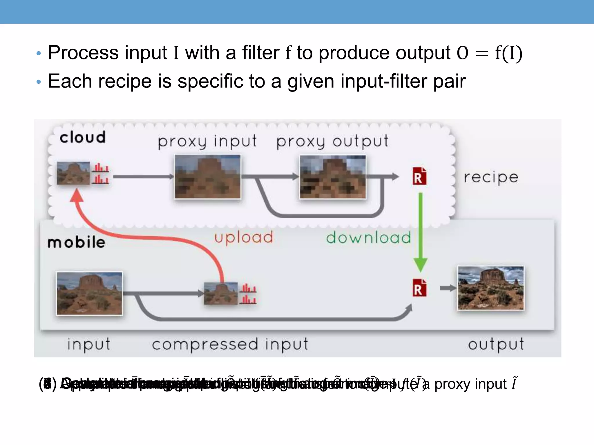
[1] Transform Recipes for Efficient Cloud Photo Enhancement
Michaël Gharbi, YiChang Shih, Gaurav Chaurasia,
Jonathan Ragan-Kelley, Sylvain Paris, Frédo Durand
SIGGRAPH ASIA 2015
[2] Data-driven Hallucination for Different Times of Day from a Single
Outdoor Photo
YiChang Shih, Sylvain Paris, Frédo Durand, William T. Freeman
SIGGRAPH ASIA 2013
[3] SLIC Superpixels Compared to State-of-the-art Superpixel Methods
Radhakrishna Achanta, Appu Shaji, Kevin Smith, Aurelien Lucchi,
Pascal Fua, and Sabine Susstrunk

40. Appendix

41. Application
Dehazing
HDR ToningColor Harmonization
Color Grading
Color Constancy Auto Colors

42. Application - Times of Day Hallucination

43. Application – Photoshop

44. Closed-form Solution
• Solution by iterative method
• 𝐴 𝑘 = 𝑣 𝑘 O 𝑣 𝑘 I 𝑇 + ϵ𝑣 𝑘 T 𝑣 𝑘 M
𝑇
+ γG
(𝑣 𝑘 I 𝑣 𝑘 I 𝑇 + ϵ𝑣 𝑘 M 𝑣 𝑘 M
𝑇
+ γId4)−1
• Define 𝐵 𝑘 = (𝑣 𝑘 I 𝑣 𝑘 I 𝑇 + ϵ𝑣 𝑘 M 𝑣 𝑘 M
𝑇
+ γId4)−1
• O = 𝑀−1 𝑢
• M = 𝑘 𝑙𝑖𝑓𝑡 𝑘 𝐼𝑑 𝑁 − 𝑣 𝑘 𝐼 𝑇 𝐵 𝑘 𝑣 𝑘 𝐼
• u = 𝑘 𝑙𝑖𝑓𝑡 𝑘((𝜖𝑣 𝑘 𝑇 𝑣 𝑘 𝑀
𝑇
+ 𝛾𝐺)𝐵 𝑘 𝑣 𝑘 𝐼 )