SlideShare a Scribd company logo
1 of 20
Download to read offline
1 m a r c h 2 0 1 8 | V O L 5 5 5 | N A T U R E | 6 7
Letter doi:10.1038/nature25792
An absorption profile centred at 78 megahertz in the
sky-averaged spectrum
Judd D. Bowman1
, Alan E. E. Rogers2
, Raul A. Monsalve1,3,4
, Thomas J. Mozdzen1
& Nivedita Mahesh1
After stars formed in the early Universe, their ultraviolet light is
expected, eventually, to have penetrated the primordial hydrogen
gas and altered the excitation state of its 21-centimetre hyperfine
line. This alteration would cause the gas to absorb photons from
the cosmic microwave background, producing a spectral distortion
that should be observable today at radio frequencies of less than
200 megahertz1
. Here we report the detection of a flattened
absorption profile in the sky-averaged radio spectrum, which is
centred at a frequency of 78 megahertz and has a best-fitting full-
width at half-maximum of 19 megahertz and an amplitude of 0.5
kelvin. The profile is largely consistent with expectations for the
21-centimetre signal induced by early stars; however, the best-fitting
amplitude of the profile is more than a factor of two greater than
the largest predictions2
. This discrepancy suggests that either the
primordial gas was much colder than expected or the background
radiation temperature was hotter than expected. Astrophysical
phenomena (such as radiation from stars and stellar remnants) are
unlikely to account for this discrepancy; of the proposed extensions
to the standard model of cosmology and particle physics, only
cooling of the gas as a result of interactions between dark matter
and baryons seems to explain the observed amplitude3
. The low-
frequency edge of the observed profile indicates that stars existed
and had produced a background of Lyman-α photons by 180 million
years after the Big Bang. The high-frequency edge indicates that
the gas was heated to above the radiation temperature less than
100 million years later.
Observations with the Experiment to Detect the Global Epoch of
Reionization Signature (EDGES) low-band instruments, which began
in August 2015, were used to detect the absorption profile. Each of the
two low-band instruments consists of a radio receiver and a zenith-­
pointing, single-polarization dipole antenna. Spectra of the brightness
temperature of the radio-frequency sky noise, spatially averaged over
the large beams of the instruments, were recorded between 50 MHz
and 100 MHz. Raw spectra were calibrated, filtered and integrated over
­hundreds of hours. Automated measurements of the reflection coeffi-
cients of the antennas were performed in the field. Other measurements
were performed in the laboratory, including of the noise waves and
reflection coefficients of the low-noise amplifiers and additional
calibration constants. Details of the instruments, calibration, verifica-
tion and model fitting are described in Methods.
In Fig. 1 we summarize the detection. It shows the spectrum
observed by one of the instruments and the results of model fits.
Galactic synchrotron emission dominates the observed sky noise,
­yielding a power-law spectral profile that decreases from about
5,000 K at 50 MHz to about 1,000 K at 100 MHz for the high Galactic
latitudes shown. Fitting and removing the Galactic emission and
ionospheric contributions from the spectrum using a five-term,
physically motivated foreground model (equation (1) in Methods)
results in a residual with a root-mean-square (r.m.s.) of 0.087 K.
The absorption profile is found by fitting the integrated spectrum
with the foreground model and a model for the 21-cm signal
simultaneously. The best-fitting 21-cm model yields a symmetric
U-shaped absorption profile that is centred at a frequency of
78 ±​ 1 MHz and has a full-width at half-­maximum of −
+
19 MHz2
4
, an
amplitude of . − .
+ .
0 5 K0 2
0 5
and a flattening factor of τ= −
+
7 3
5
(where the
bounds provide 99% confidence intervals including estimates of
systematic uncertainties; see Methods for model definition).
Uncertainties in the parameters of the fitted profile are estimated
from statistical uncertainty in the model fits and from ­systematic
differences between the various validation trials that were performed
using observations from both instruments and several ­different data
cuts. The 99% confidence intervals that we report are calculated as
the outer bounds of (1) the marginalized statistical 99% confidence
intervals from fits to the primary dataset and (2) the range of best-
fitting values for each parameter across the validation trials. Fitting
with both the foreground and 21-cm models lowers the residuals to
an r.m.s. of 0.025 K. The fit shown in Fig. 1 has a signal-to-noise ratio
of 37, calculated as the best-fitting amplitude of the profile divided
by the statistical uncertainty of the amplitude fit, including the cova­
riance between model parameters. Additional analyses of the
1
School of Earth and Space Exploration, Arizona State University, Tempe, Arizona 85287, USA. 2
Haystack Observatory, Massachusetts Institute of Technology, Westford, Massachusetts 01886, USA.
3
Center for Astrophysics and Space Astronomy, University of Colorado, Boulder, Colorado 80309, USA. 4
Facultad de Ingeniería, Universidad Católica de la Santísima Concepción, Alonso de Ribera
2850, Concepción, Chile.
1,000
3,000
5,000
Temperature,T(K)
a
50 60 70 80 90 100
–0.2
0
0.2
Temperature,T(K)
b
r.m.s. = 0.087 K
c
r.m.s. = 0.025 K
50 60 70 80 90 10050 60 70 80 90 100
–0.6
–0.4
–0.2
0
d
Temperature,T(K)
50 60 70 80 90 10050 60 70 80 90 100
Frequency, (MHz)Frequency, (MHz)
e
Figure 1 | Summary of detection. a, Measured spectrum for the reference
dataset after filtering for data quality and radio-frequency interference.
The spectrum is dominated by Galactic synchrotron emission.
b, c, Residuals after fitting and removing only the foreground
model (b) or the foreground and 21-cm models (c). d, Recovered
model profile of the 21-cm absorption, with a signal-to-noise
ratio of 37, amplitude of 0.53 K, centre frequency of 78.1 MHz and
width of 18.7 MHz. e, Sum of the 21-cm model (d) and its residuals (c).
© 2018 Macmillan Publishers Limited, part of Springer Nature. All rights reserved.
6 8 | N A T U R E | V O L 5 5 5 | 1 m a r c h 2 0 1 8
LetterRESEARCH
observations using restricted spectral bands yield nearly identical
best-fitting absorption profiles, with the highest signal-to-noise ratio
reaching 52. In Fig. 2 we show representative cases of these fits.
We performed numerous hardware and processing tests to validate
the detection. The 21-cm absorption profile is observed in data that
span nearly two years and can be extracted at all local solar times and
at all local sidereal times. It is detected by two identically designed
instruments operated at the same site and located 150 m apart, and
even after several hardware modifications to the instruments, includ-
ing orthogonal orientations of one of the antennas. Similar results for
the absorption profile are obtained by using two independent pro-
cessing pipelines, which we tested using simulated data. The profile is
detected using data processed via two different calibration techniques:
absolute calibration and an additional differencing-based post-
calibration process that reduces some possible instrumental errors. It
is also detected using several sets of calibration solutions derived from
­multiple laboratory measurements of the receivers and using ­multiple
on-site measurements of the reflection coefficients of the antennas.
We modelled the sensitivity of the detection to several possible
calibration errors and in all cases recovered profile amplitudes that
are within the reported confidence range, as summarized in Table 1.
An EDGES high-band instrument operates between 90 MHz and
200 MHz at the same site using a nearly identical receiver and a scaled
version of the low-band antennas. It does not produce a similar ­feature
at the scaled frequencies4
. Analysis of radio-frequency interference
in the observations, including in the FM radio band, shows that
the absorption profile is inconsistent with typical spectral contribu-
tions from these sources.
We are not aware of any alternative astronomical or atmospheric
mechanisms that are capable of producing the observed profile. H ii
regions in the Galaxy have increasing optical depth with wavelength,
blocking more background emission at lower frequencies, but they
are observed primarily along the Galactic plane and generate mono-
tonic spectral profiles at the observed frequencies. Radio-frequency
recombination lines in the Galactic plane create a ‘picket fence’ of
narrow absorption lines separated by approximately 0.5 MHz at the
observed frequencies5
, but these lines are easy to identify and filter
in the EDGES observations. The Earth’s ionosphere weakly absorbs
radio signals at the observed frequencies and emits thermal radiation
from hot electrons, but models and observations imply a broadband
effect that varies depending on the ionospheric conditions6,7
, including
diurnal changes in the total electron content. This effect is fitted by
our foreground model. Molecules of the hydroxyl radical and nitric
oxide have spectral lines in the observed band and are present in the
atmosphere, but the densities and line strengths are too low to produce
substantial absorption.
The 21-cm line has a rest-frame frequency of 1,420 MHz. Expansion
of the Universe redshifts the line to the observed band according to
ν =​ 1,420/(1 +​ z) MHz, where z is the redshift, which maps uniquely
to the age of the Universe. The observed absorption profile is the con-
tinuous superposition of lines from gas across the observed redshift
range and cosmological volume; hence, the shape of the profile traces
the history of the gas across cosmic time and is not the result of the
properties of an individual cloud. The observed absorption profile is
centred at z ≈​ 17 and spans approximately 20 >​ z >​ 15.
The intensity of the observable 21-cm signal from the early
Universe is given as a brightness temperature relative to the micro-
wave background8
:
Ω
Ω
≈ . ×







. 





+ 








 .







−




T z x z
z h T z
T z
( ) 0 023 K ( )
0 15 1
10 0 02
1
( )
( )
21 H
m
1
2
b R
S
I
where xHi is the fraction of neutral hydrogen, Ωm and Ωb are the matter
and baryon densities, respectively, in units of the critical density for a
flat universe, h is the Hubble constant in units of 100 km s−1
 Mpc−1
,
TR is the temperature of the background radiation, usually assumed to
be from the background produced by the afterglow of the Big Bang,
TS is the 21-cm spin temperature that defines the relative population
of the hyperfine energy levels, and the factor of 0.023 K comes from
atomic-line physics and the average gas density. The spin temperature
is affected by the absorption of microwave photons, which couples TS
to TR, as well as by resonant scattering of Lyman-α​photons and atomic
collisions, both of which couple TS to the kinetic temperature of the
gas TG.
The temperatures of the gas and the background radiation are
­coupled in the early Universe through Compton scattering. This
­coupling becomes ineffective in numerical models9,10
at z ≈​ 150,
after which primordial gas cools adiabatically. In the absence of
stars or non-standard physics, the gas temperature is expected to be
9.3 K at z =​ 20, falling to 5.4 K at z =​ 15. The radiation temperature
decreases more slowly owing to cosmological expansion, following
T0(1 + z) with T0 =​ 2.725, and so is 57.2 K and 43.6 K at the same
redshifts, ­respectively. The spin temperature is initially coupled to the
gas temperature as the gas cools below the radiation temperature, but
eventually the decreasing density of the gas is insufficient to main-
tain this coupling and the spin temperature returns to the radiation
temperature.
Redshift, z
14161820222426
Brightnesstemperature,T21(K)
–0.6
–0.4
–0.2
0
0.2
H1
H2
H3
H4
H5
H6
P8
Age of the Universe (Myr)
300250200150
Figure 2 | Best-fitting 21-cm absorption profiles for each hardware case.
Each profile for the brightness temperature T21 is added to its residuals and
plotted against the redshift z and the corresponding age of the Universe.
The thick black line is the model fit for the hardware and analysis
configuration with the highest signal-to-noise ratio (equal to 52; H2;
see Methods), processed using 60–99 MHz and a four-term polynomial
(see equation (2) in Methods) for the foreground model. The thin solid
lines are the best fits from each of the other hardware configurations
(H1, H3–H6). The dash-dotted line (P8), which extends to z >​ 26, is
reproduced from Fig. 1e and uses the same data as for the thick black line
(H2), but a different foreground model and the full frequency band.
Table 1 | Sensitivity to possible calibration errors
Error source
Estimated
uncertainty
Modelled
error level
Recovered
amplitude (K)
LNA S11 magnitude 0.1 dB 1.0 dB 0.51
LNA S11 phase (delay) 20 ps 100 ps 0.48
Antenna S11 magnitude 0.02 dB 0.2 dB 0.50
Antenna S11 phase (delay) 20 ps 100 ps 0.48
No loss correction N/A N/A 0.51
No beam correction N/A N/A 0.48
The estimated uncertainty for each case is based on empirical values from laboratory
­measurements and repeatability tests. Modelled error levels were chosen conservatively to
be five and ten times larger than the estimated uncertainties for the phases and magnitudes,
­respectively. LNA, low-noise amplifier; S11, input reflection coefficient; N/A, not applicable.
© 2018 Macmillan Publishers Limited, part of Springer Nature. All rights reserved.
1 m a r c h 2 0 1 8 | V O L 5 5 5 | N A T U R E | 6 9
Letter RESEARCH
Over time, Lyman-α​photons from early stars recouple the spin and
gas temperatures11
, leading to the detected signal. The onset of the
observed absorption profile at z =​ 20 places this epoch at an age of
180 million years, using the Planck 2015 cosmological parameters12
.
For the most extreme case, in which TS is fully coupled to TG, the gas
and radiation temperatures calculated here yield a maximum absorp-
tion amplitude of 0.20 K at z =​ 20, which increases to 0.23 K at z =​ 15.
The presence of stars should eventually halt the cooling of the gas
and ultimately heat it, because stellar radiation deposits energy into
the gas and Lyman-line cooling has been modelled to be very small for
the expected stellar properties13
. As early stars die, they are expected
to leave behind stellar remnants, such as black holes and neutron stars.
The accretion disks around these remnants should generate X-rays,
further heating the gas. At some point, the gas is expected to become
hotter than the background radiation temperature, ending the absorp-
tion signal. The z =​ 15 edge of the observed profile places this transition
around 270 million years after the Big Bang.
The ages derived for the events above fall within the range expected
from many theoretical models2
. However, the flattened shape of the
observed absorption profile is uncommon in existing models, and
could indicate that the initial flux of Lyman-α​radiation from early stars
was sufficiently large that the spin temperature saturated quickly to the
gas temperature. We analysed models that assume a high Lyman-α​ flux
at z <​ 14 using the EDGES high-band measurements and found a large
fraction to be inconsistent with the data4
.
To produce the best-fitting profile amplitude of 0.5 K, the ratio
TR/TS at the centre of the profile must be larger than 15, compared to
a ­maximum of 7 allowed by the gas and radiation temperatures stated
above. Even the lower confidence bound of 0.3 K for the observed
­profile amplitude is roughly 50% larger than the strongest predicted
signal. For a standard gas temperature history, TR would need to be
more than 104 K to yield the best-fitting amplitude at the centre of the
profile, whereas for a radiation temperature history given solely by the
microwave background, TG would need to be less than 3.2 K.
The observed profile amplitude could be explained if the gas and
background radiation temperatures decoupled by z ≈​ 250 rather
than z ≈​ 150, allowing the gas to begin cooling adiabatically earlier.
A ­residual ionization fraction after the formation of atoms that is less
than the expected fraction by nearly an order of magnitude would lead
to sufficiently early decoupling. However, cross-validation between
numerical models and their consistency with Planck observations
­suggest that the residual ionization fraction is already known to
approxi­mately 1% fractional accuracy.
Considering more exotic scenarios, interactions between dark matter
and baryons can explain the observed profile amplitude (by lowering
the gas temperature14
) if the mass of dark-matter particles is below a
few gigaelectronvolts and the interaction cross-section is greater than
about 10−21
 cm2
(ref. 3). Existing models of other non-standard physics,
including dark-matter decay and annihilation15
, accreting or evapo-
rating primordial black holes16
, and primordial magnetic fields17
, all
predict increased gas temperatures and are unlikely to account for the
observed amplitude. It is possible that some of these sources could also
increase TR through mechanisms such as synchrotron emission associ-
ated with primordial black holes18
or the relativistic electrons that result
from the decay of metastable particles19
, but it is unclear whether this
could compensate for the increased gas temperature. Measurements
from ARCADE-2 (ref. 20) suggest an isotropic radio background that
cannot be explained by known source populations, but this interpre-
tation is still debated21
and the unknown sources would need to be
present at z ≈​ 20 to affect the radiation environment relevant to the
observed signal.
Although we have performed many tests to be confident that the
observed profile is from a global absorption of the microwave back-
ground by hydrogen gas in the early Universe, we still seek confirma-
tion observations from other instruments. Several experiments similar
to EDGES are underway. Those closest to achieving the performance
required to verify the profile include the Large-Aperture Experiment
to Detect the Dark Ages (LEDA)22
, the Sonda Cosmológica de las Islas
para la Detección de Hidrógeno Neutro (SCI-HI)23
, the Probing Radio
Intensity at high z from Marion (PRIZM) and the Shaped Antenna
measurement of the background Radio Spectrum 2 (SARAS 2)24
. The
use of more sophisticated foreground models than we have used could
lower the performance requirements of the hardware, and could lead
to better profile recovery because low-order (smooth) modes in any
fitted profile shape tend to be covariant with our foreground model and
so are potentially under-constrained. Singular-value decomposition of
training sets constructed from simulated instrument error terms and
foreground contributions can produce optimized basis sets for model
fitting25,26
. We plan to apply these techniques to our data ­processing.
The best measurement of the observed profile might ultimately be
conducted in space, where the Earth’s atmosphere and ionosphere
­cannot influence the propagation of the astronomical signal, poten-
tially reducing the burden of the foreground model. The measurement
could be made from the lunar farside27
—either on the surface or from
an orbit around the Moon—using the Moon as a shield to block FM
radio ­signals and other Earth-based transmitters.
This result should bolster ongoing efforts to detect the statistical
properties of spatial fluctuations in the 21-cm signal using inter-
ferometric arrays; it provides direct evidence that a signal exists for
these telescopes to detect. The Hydrogen Epoch of Reionization
Array28
(HERA) will become operational over the next two years and
will be able to characterize the power spectrum of redshifted 21-cm
fluctuations between 100 MHz and 200 MHz during the epoch of reion-
ization, when the 21-cm signal should be visible as emission above the
background. The operational band of HERA is also expected to be
extended to 50 MHz over this time. HERA will probably have suffi-
cient thermal sensitivity to detect any power-spectrum signal associ-
ated with the EDGES observed profile and so might be able to validate
the absorption signal reported here. But foregrounds have proven to
be more challenging for interferometers than expected, and sufficient
foreground mitigation to detect the 21-cm power spectrum has yet to
be demonstrated by any of the currently operating arrays, including
the Low-Frequency Array (LOFAR)29
and the Murchison Widefield
Array (MWA)30
. Expansion of an ­existing Long Wavelength Array31
station would provide the sensitivity necessary to pursue power-
spectrum detection. When constructed, the Square Kilometre Array
(SKA) Low-Frequency Aperture Array (https://www.skatelescope.org)
should be able to detect the power spectrum associated with the absorp-
tion profile reported here and, eventually, to image the 21-cm signal.
Online Content Methods, along with any additional Extended Data display items and
Source Data, are available in the online version of the paper; references unique to
these sections appear only in the online paper.
received 13 September 2017; accepted 24 January 2018.
1.	 Pritchard, J. R. & Loeb, A. 21 cm cosmology in the 21st century. Rep. Prog.
Phys. 75, 086901 (2012).
2.	 Cohen, A., Fialkov, A., Barkana, R. & Lotem, M. Charting the parameter
space of the global 21-cm signal. Mon. Not. R. Astron. Soc. 472, 1915–1931
(2017).
3.	 Barkana, R. Possible interaction between baryons and dark-matter particles
revealed by the first stars. Nature 555, https://doi.org/10.1038/nature25791
(2018).
4.	 Monsalve, R. A., Rogers, A. E. E., Bowman, J. D. & Mozdzen, T. J. Results from
EDGES high-band. I. Constraints on phenomenological models for the global
21 cm signal. Astrophys. J. 847, 64 (2017).
5.	 Alves, M. I. R. et al. The HIPASS survey of the Galactic plane in radio
recombination lines. Mon. Not. R. Astron. Soc. 450, 2025–2042 (2015).
6.	 Rogers, A. E. E., Bowman, J. D., Vierinen, J., Monsalve, R. A. & Mozdzen, T.
Radiometric measurements of electron temperature and opacity of
ionospheric perturbations. Radio Sci. 50, 130–137 (2015).
7.	 Sokolowski, M. et al. The impact of the ionosphere on ground-based detection
of the global epoch of reionization signal. Astrophys. J. 813, 18 (2015).
8.	 Zaldarriaga, M., Furlanetto, S. R. & Hernquist, L. 21 centimeter fluctuations
from cosmic gas at high redshifts. Astrophys. J. 608, 622–635 (2004).
9.	 Ali-Haïmoud, Y. & Hirata, C. M. HyRec: a fast and highly accurate primordial
hydrogen and helium recombination code. Phys. Rev. D 83, 043513 (2011).
© 2018 Macmillan Publishers Limited, part of Springer Nature. All rights reserved.
7 0 | N A T U R E | V O L 5 5 5 | 1 m a r c h 2 0 1 8
LetterRESEARCH
10.	 Shaw, J. R. & Chluba, J. Precise cosmological parameter estimation using
COSMOREC. Mon. Not. R. Astron. Soc. 415, 1343–1354 (2011).
11.	 Furlanetto, S. R. The global 21-centimeter background from high redshifts.
Mon. Not. R. Astron. Soc. 371, 867–878 (2006).
12.	 Planck Collaboration. Planck 2015 results. XIII. Cosmological parameters.
Astron. Astrophys. 594, A13 (2016).
13.	 Chen, X. & Miralda-Escude, J. The spin-kinetic temperature coupling and the
heating rate due to Lyα​scattering before reionization: predictions for 21
centimeter emission and absorption. Astrophys. J. 602, 1–11 (2004).
14.	 Tashiro, H., Kadota, K. & Silk, J. Effects of dark matter-baryon scattering on
redshifted 21 cm signals. Phys. Rev. D 90, 083522 (2014).
15.	 Lopez-Honorez, L., Mena, O., Moliné, Á., Palomares-Ruiz, S. & Vincent, A. C.
The 21 cm signal and the interplay between dark matter annihilations and
astrophysical processes. J. Cosmol. Astropart. Phys. 8, 4 (2016).
16.	 Tashiro, H. & Sugiyama, N. The effect of primordial black holes on 21-cm
fluctuations. Mon. Not. R. Astron. Soc. 435, 3001–3008 (2013).
17.	 Schleicher, D. R. G., Banerjee, R. & Klessen, R. S. Influence of primordial
magnetic fields on 21 cm emission. Astrophys. J. 692, 236–245 (2009).
18.	 Biermann, P. L. et al. Cosmic backgrounds due to the formation of the first
generation of supermassive black holes. Mon. Not. R. Astron. Soc. 441,
1147–1156 (2014).
19.	 Cline, J. M. & Vincent, A. C. Cosmological origin of anomalous radio
background. J. Cosmol. Astropart. Phys. 2, 11 (2013).
20.	 Seiffert, M. et al. Interpretation of the Arcade 2 absolute sky brightness
measurement. Astrophys. J. 734, 6 (2011).
21.	 Vernstrom, T., Norris, R. P., Scott, D. & Wall, J. V. The deep diffuse
extragalactic radio sky at 1.75 GHz. Mon. Not. R. Astron. Soc. 447,
2243–2260 (2015).
22.	 Bernardi, G. et al. Bayesian constraints on the global 21-cm signal from the
cosmic dawn. Mon. Not. R. Astron. Soc. 461, 2847–2855 (2016).
23.	 Voytek, T. C., Natarajan, A., Jáuregui García, J. M., Peterson, J. B. & López-Cruz,
O. Probing the dark ages at z ~​20: the SCI-HI 21 cm all-sky spectrum
experiment. Astrophys. J. 782, L9 (2014).
24.	 Singh, S. et al. First results on the epoch of reionization from first light with
SARAS 2. Astrophys. J. 845, L12 (2017).
25.	 Switzer, E. R. & Liu, A. Erasing the variable: empirical foreground
discovery for global 21 cm spectrum experiments. Astrophys. J. 793, 102
(2014).
26.	 Vedantham, H. K. et al. Chromatic effects in the 21 cm global signal from the
cosmic dawn. Mon. Not. R. Astron. Soc. 437, 1056–1069 (2014).
Acknowledgements We thank CSIRO for providing site infrastructure and
access to facilities. We thank the MRO Support Facility team, especially M. Reay,
L. Puls, J. Morris, S. Jackson, B. Hiscock and K. Ferguson. We thank C. Bowman,
D. Cele, C. Eckert, L. Johnson, M. Goodrich, H. Mani, J. Traffie and K. Wilson for
instrument contributions. We thank R. Barkana for theory contributions and
G. Holder, T. Vachaspati, C. Hirata and J. Chluba for exchanges. We thank
C. Lonsdale, H. Johnson, J. Hewitt and J. Burns. We thank C. Halleen and
M. Halleen for site and logistical support. This work was supported by the
NSF through awards AST-0905990, AST-1207761 and AST-1609450. R.A.M.
acknowledges support from the NASA Ames Research Center (NNX16AF59G)
and the NASA Solar System Exploration Research Virtual Institute
(80ARC017M0006). This work makes use of the Murchison Radio-astronomy
Observatory. We acknowledge the Wajarri Yamatji people as the traditional
owners of the site of the observatory.
Author Contributions J.D.B., R.A.M. and A.E.E.R. contributed to all activities. N.M.
and T.J.M. modelled instrument properties, performed laboratory calibrations
and contributed to the preparation of the manuscript.
Author Information Reprints and permissions information is available at
www.nature.com/reprints. The authors declare no competing financial
interests. Readers are welcome to comment on the online version of the paper.
Publisher’s note: Springer Nature remains neutral with regard to jurisdictional
claims in published maps and institutional affiliations. Correspondence and
requests for materials should be addressed to J.D.B. (judd.bowman@asu.edu).
Reviewer Information Nature thanks S. Weinreb and the other anonymous
reviewer(s) for their contribution to the peer review of this work.
27.	 Burns, J. O. et al. A space-based observational strategy for characterizing the
first stars and galaxies using the redshifted 21 cm global spectrum.
Astrophys. J. 844, 33 (2017).
28.	 DeBoer, D. R. et al. Hydrogen Epoch of Reionization Array (HERA). Publ. Astron.
Soc. Pac. 129, 045001 (2017).
29.	 Patil, A. H. et al. Upper limits on the 21 cm epoch of reionization power
spectrum from one night with LOFAR. Astrophys. J. 838, 65 (2017).
30.	 Beardsley, A. P. et al. First season MWA EoR power spectrum results at
redshift 7. Astrophys. J. 833, 102 (2016).
31.	 Dowell, J., Taylor, G. B., Schinzel, F. K., Kassim, N. E. & Stovall, K. The LWA1 low
frequency sky survey. Mon. Not. R. Astron. Soc. 469, 4537–4550 (2017).
© 2018 Macmillan Publishers Limited, part of Springer Nature. All rights reserved.
Letter RESEARCH
Methods
Instrument. The EDGES experiment is located at the Murchison Radio-astronomy
Observatory (MRO) in Western Australia (26.72° S, 116.61° E), which is the
same radio-quiet32
site used by the Australian SKA precursor, the Murchison
Widefield Array and the planned SKA Low-Frequency Aperture Array. An
early version of EDGES placed an empirical lower limit on the duration of the
epoch of reionization33
. EDGES currently consists of three instruments: a high-
band instrument4,34,35
that is sensitive to 90–200 MHz (14 >​ z >​ 6) and two low-
band instruments (low-1 and low-2) that operate over the range 50–100 MHz
(27 >​ z >​ 13). Each instrument yields spectra with 6.1-kHz resolution. In each
instrument, sky radiation is collected by a wideband dipole-like antenna that
­consists of two rectangular metal panels mounted horizontally above a metal
ground plane. Similar compact dipole antennas are used elsewhere in radio
­astronomy36,37
. A receiver is installed underneath the ground plane and a balun38
is used to guide radiation from the antenna panels to the receiver. A rectangular
shroud surrounds the base of the balun to shield the vertical currents in the balun
tubes, which are strongest at the base. This lowers the gain towards the horizon
owing to the vertical currents.
Extended Data Fig. 1 shows a block diagram of the system. A mechanical input
switch at the front of the receiver enables the antenna to be connected to a remote
vector network analyser (VNA) to measure the antenna reflection coefficients
accurately or to be connected to the primary receiver path to measure the sky
noise spectrum. When measuring the sky noise spectrum a second ­mechanical
switch connects the low-noise amplifier (LNA) to the antenna or to a 26-dB
attenuator, which acts as a load or a well matched noise source, depending on the
state of the electrical switch on the noise source. This performs a three-position
switching operation39
between ambient and ‘hot’ internal noise sources and the
antenna, which is needed to provide the first stage of processing discussed below.
After the LNA and post-amplifier, another noise source is used to inject noise
at less than 45 MHz. This ‘out of band’ conditioning improves the linearity and
dynamic range of the analogue-to-digital converter (ADC), which are needed for
the ­accurate ­cancellation of the receiver bandpass that is afforded by the three-­
position ­switching. A thermoelectric system maintains a constant temperature
in the receiver in the field and in the laboratory. The system mitigates against
radio-­frequency interference (RFI) using designs and analysis strategies adapted
from the Deuterium Array40
. Similar approaches to instrument design are used
for SARAS 2 (ref. 41) and LEDA42
.
The design of the low-band instrument differs from the published descriptions
of the design of the high-band instrument only by the following. First, a 3-dB
attenuator is added within the LNA before the pseudomorphic high-electron-
mobility transistor at the input. The attenuator improves the LNA impedance
match and thereby reduces the sensitivity to measurement errors of the LNA
and antenna reflection coefficients, especially to errors in the reflection phase,
while adding only a small amount of noise compared with the sky noise. Larger
values of attenuation would begin to add substantial noise at 100 MHz. Second,
a scaled antenna is used that is precisely double the size of the antenna of the
high-band instrument. Third, a larger ground plane is used. Each ground plane
of the low-band instrument consists of a 2 m ×​ 2 m solid metal central assembly
surrounded by metal mesh that spans 30 m ×​ 30 m, with the outer 5 m shaped
as saw-tooth perforated edges. Low-1 was initially operated with a 10 m ×​ 10 m
ground plane and later extended to full size. The full-size 30 m ×​ 30 m ground
plane reduces the chromaticity of the beam and makes it less sensitive to con-
ditions of the soil. Extended Data Fig. 2 shows the low-1 and low-2 antennas,
Extended Data Fig. 3 the measured reflection coefficients and Extended Data
Fig. 4 cuts through the model of the antenna beam pattern.
Calibration. We implement end-to-end absolute calibration for the low-band
instruments following the techniques developed for the high-band instrument34,43
.
The calibration procedure involves taking reference spectra in the laboratory with
the receiver connected to hot and ambient loads and to open and shorted cables.
Similar techniques are used in other microwave measurements44,45
. Reflection
coefficient measurements using a VNA are acquired for the calibration sources
and the LNA. The input connection to the receiver box provides the reference
plane for all VNA measurements. To correct for the losses in the hot load used
in the laboratory for calibration, full scattering parameters are measured for the
short cable from the heated resistor in the hot load. The accuracy of scattering
parameter measurements is improved by accounting for the actual resistance of
the 50-Ω​load used for VNA calibration and the added inductance in the load due
to skin effects46
in the few millimetres of transmission line between its internal
termination and the reference plane47
.
The calibration spectra and reflection coefficient measurements acquired in the
laboratory are used to solve for the free parameters34
in the equations that account
for the impedance mismatches between the receiver and the antenna and for the
correlated and uncorrelated LNA noise waves. Laboratory calibration is performed
with the receiver temperature controlled to the default 25 °C, and at 15 °C and 35 °C
to assess the thermal dependence of the calibration parameters. Extended Data Fig. 5
shows calibration parameter solutions for both receivers.
Following calibration in the laboratory, a test is performed by measuring the
spectrum of an approximately 300 K passive load with deliberate impedance
­mismatch that approximately mimics the reflection from the antenna in magnitude
and phase. We call this device an ‘artificial antenna simulator’. The reflection
coefficient of the antenna simulator is measured and applied to yield calibrated
integrated spectra. Extended Data Fig. 3 shows measured reflection coefficients for
the artificial antenna simulator. Once corrected, the integrated spectra are expected
to be spectrally flat, with a noise temperature that matches the physical temperature
of the passive load. The flatness of an integrated spectrum is quantified through
the r.m.s. of the residuals after subtracting a constant term. The typical r.m.s. of
the ­residuals is 0.025 K over the range 50–100 MHz. If a three-term polynomial
(equation (2) with N =​ 3) is subtracted, then the residuals decrease to about 0.015 K
and are limited by integration time.
A second test of the calibration is performed by measuring the spectrum of a
noise source followed by a filter and an approximately 3-m cable that adds about
30 ns of two-way delay. The device yields a spectrum that is similar in shape to
the sky foreground with a strength of about 10,000 K (seven times larger than
the ­typical sky temperature observed by EDGES) at 75 MHz and has a reflection
coefficient of −​6 dB in magnitude with a phase slope similar to that of the antenna.
Typical residuals are less than 300 mK after subtracting a five-term polynomial
(equation (2)) and are limited by integration time. Assuming any residuals scale
with input power, this value corresponds to residuals of 45 mK at the typical
observed sky temperature. This test is more sensitive than the passive ­simulator,
especially to errors in the measurements of the reflection coefficient, because
the signal is 33 times stronger than that of the approximately 300-K load and
because the magnitude of the reflection of this simulator is larger than that of the
passive simulator and of the real antenna.
Losses in the balun and losses due to the finite ground plane are corrected for
during data processing using models. The balun-loss model is validated against
scattering parameter measurements. Frequency-dependent beam effects are com-
pensated for by modelling and subtracting the spectral structure using electro­
magnetic beam models and a diffuse sky map template35
. The nominal beam model
accounts for the finite metal ground plane over soil with a relative permittivity of
3.5 and conductivity of 2 ×​ 10−2
 S m−1
(ref. 48). The sky template is produced by
extrapolating the 408-MHz all-sky radio map49
to the observed frequencies using
a spectral index in brightness temperature of −​2.5 (refs 35, 43).
Data and processing. Examples of raw and processed data are shown in Extended
Data Fig. 6. Data processing involves three primary stages. In the first stage, three
raw spectra that have each been accumulated for 13 s from the antenna input
and two internal reference noise sources are converted into a single ­partially
­calibrated spectrum39
. Individual 6.1-kHz channels above a fixed power threshold
are assigned zero weight to remove RFI. The threshold is normally set at three
times the r.m.s. of the residuals after substacting a constant and a slope in a ­sliding
256-spectral-channel window. Similarly, any partially calibrated spectrum with
an ­average power above that expected from the sky or with large residuals is
­discarded. A weighted average of many successive spectra is taken, typically over
several hours. Outlier channels after a Fourier series fit to the entire accumulated
spectrum are again assigned zero weight. This second pass assigns zero weight to
lower levels of RFI and broader RFI signals than does the initial pass.
Inthesecondstageofprocessing,thepartiallycalibratedspectraarefullycalibrated
usingthecalibrationparametersfromthelaboratoryandtheantennareflectioncoef-
ficient measurements taken periodically in the field. Beam-chromaticity corrections
areappliedafteraveragingthemodeloverthesamerangeoflocalsiderealtimesasfor
the spectra. The spectra are then corrected for the balun and ground-plane loss and
output with a typical smoothing to spectral bins with 390.6-kHz resolution.
In the third stage of processing, spectra for each block of local sidereal time of
several hours within each day are fitted with a foreground model (see below for
description of models). An r.m.s. value of the residuals is computed for each block
and blocks above a selected threshold are discarded, typically because of broad-
band RFI—or solar activity in daytime data—that was not detected in the earlier
processing stages. A weighted average is then taken of the accepted blocks and a
weighted least-squares solution is determined using a foreground model along
with the model that represents the 21-cm absorption signal. Extended Data Fig. 7
shows the final weights for each spectral bin, equivalent to the RFI occupancy.
The observations used for the primary analysis presented here are from low-1,
spanning 2016 day 252 through to 2017 day 94 (configuration H2 below). The
data are filtered to retain only local Galactic hour angles (GHA) of 6–18 h; GHA
is equivalent to the local sidereal time offset by 17.75 h.
© 2018 Macmillan Publishers Limited, part of Springer Nature. All rights reserved.
LetterRESEARCH
Parameter estimation. The polynomial foreground model used for the analysis
presented in Fig. 1 is physically motivated, with five terms based on the known
spectral properties of the Galactic synchrotron spectrum and Earth’s ionosphere6,50
:
ν
ν
ν
ν
ν
ν
ν
ν
ν
ν
ν
ν
ν
ν
ν
≈






+












+




















+





 +






− . − . − .
− . −
T a a a
a a
( ) log log
(1)
F 0
c
2 5
1
c
2 5
c
2
c
2 5
c
2
3
c
4 5
4
c
2
where TF(ν) is the brightness temperature of the foreground emission, ν is ­the
frequency, νc is the centre frequency of the observed band and the coefficients an
are fitted to the data. The above function is a linear approximation, centred on νc, to
ν
ν
ν
ν
ν
=






+






ν ν
ν ν
− . + + /
− /
−
−
T b b( ) e
b b
b
F 0
c
2 5 log( )
( )
4
c
21 2 c
3 c
2
which is connected directly to the physics of the foreground and the ionosphere.
The factor of −​2.5 in the first exponent is the typical power-law spectral index of
the foreground, b0 is an overall foreground scale factor, b1 allows for a correction
to the typical spectral index of the foreground (which varies by roughly 0.1 across
the sky) and b2 captures any contributions from a higher-order foreground spectral
term51,52
. Ionospheric contributions are contained in b3 and b4, which allow for the
ionospheric absorption of the foreground and emission from hot electrons in the
ionosphere, respectively. This model can also partially capture some instrumental
effects, such as additional spectral structure from chromatic beams or small errors
in calibration.
We also use a more general polynomial model in many of our trials that enables
us to explore signal recovery with varying numbers of polynomial terms:
∑ν ν=
=
−
− .T a( ) (2)
n
N
n
n
F
0
1
2 5
where N is the number of terms and the coefficients an are again fitted to the
data. As with the physical model, the −​2.5 in the exponent makes it easier for the
model to match the foreground spectrum. Both foreground models yield consistent
absorption profile results.
The 21-cm absorption profile is modelled as a flattened Gaussian:
ν = −



−
−



τ
τ
−
−
T A( )
1 e
1 e
21
eB
where
ν ν
τ
=
− 



−



+ 






τ−
B
w
4( )
log
1
log
1 e
2
0
2
2
and A is the absorption amplitude, ν0 is the centre frequency, w is the full-width at
half-maximum and τ is a flattening factor. This model is not a description of the
physics that creates the 21-cm absorption profile, but rather is a suitable functional
form to capture the basic shape of the profile. Extended Data Fig. 8 shows the
best-fitting profile and residuals from fits by the two foreground models.
We report parameter fits from a gridded search over the parameters ν0, w and
τ in the 21-cm model. For each step in the grid, we conduct a linear weighted
least-squares fit, solving simultaneously for the foreground coefficients and the
amplitude of the absorption profile. The best-fitting absorption profile maximizes
the signal-to-noise ratio in the gridded search. The uncertainty in the amplitude
fit accounts for covariance between the foreground coefficients and the amplitude
of the profile and for noise.
Fitting both foreground and 21-cm models simultaneously yields residuals that
decrease with integration time with an approximately noise-like ( / t1 ) trend for
the duration of the observation, whereas fitting only the foreground model yields
residuals that decrease with time for the first approximately 10% of the integration
and then saturate, as shown in Extended Data Fig. 9.
We also performed a Markov chain Monte Carlo (MCMC) analysis (Extended
Data Fig. 10) for the H2 case using a five-term polynomial (equation (2)) for the
foreground model and a subset of the band covering 60–94 MHz. The amplitude
parameter is most covariant with the flattening. The 99% statistical confidence
intervals on the four 21-cm model parameters are: = . − .
+ .
A 0 52 K0 18
0 42
,
ν = . − .
+ .
78 3 MHz0 0 3
0 2
, = . − .
+ .
w 20 7 MHz0 7
0 8
and τ = . − .
+ .
6 5 2 5
5 6
. These intervals do not
include any systematic error from differences across the hardware configurations
and processing trials. When the flattening parameter is fixed to τ =​ 7, statistical
uncertainty in the 21-cm model amplitude fit is reduced to approximately ±​0.02 K.
Extended Data Table 1 shows that the various hardware configurations and
­processing trials with fixed τ =​ 7 yield best-fitting parameter ranges of
0.37 K <​ A <​ 0.67 K, 77.4 MHz <​ ν0 <​ 78.5 MHz and 17.0 MHz <​ w <​ 22.8 MHz.
This systematic variation is probably due to the limited data in the some of the
configurations, small calibration errors and residual chromatic beam effects, and
potentially to structure in the Galactic foreground that increases when the Galactic
plane is overhead. For each parameter, taking the outer bounds of the statistical
confidence ranges from the comprehensive MCMC analysis for H2 and the best-­
fitting variations between validation trials in Extended Data Table 1 yields the
estimate of the 99% confidence intervals that we report in the main text.
Verification tests. Here we list the tests that we performed to verify the ­detection.
The absorption profile is detected from data obtained in the following hard-
ware configurations: H1, low-1 with 10 m ×​ 10 m ground plane; H2, low-1
with 30 m ×​ 30 m ground plane; H3, low-1 with 30 m ×​ 30 m ground plane and
­recalibrated receiver; H4, low-2 with north–south dipole orientation; H5, low-2
with east–west dipole orientation; and H6, low-2 with east–west dipole orientation
and the balun shield removed to check for any resonance that might result from a
slot antenna being formed in the joint between the two halves of the shield.
The absorption profile is detected in data processed with the following
­configurations: P1, all hardware cases, using two independent processing ­pipelines;
P2, all hardware cases, divided into temporal subsets; P3, all hardware cases, with
chromatic beam corrections on or off; P4, all hardware cases, with ground loss
and balun loss corrections on or off; P5, all hardware cases, calibrated with four
different antenna reflection coefficient measurements; P6, all hardware cases, using
a four-term foreground model (equation (2)) over the frequency range 60–99 MHz;
P7, all hardware cases, using a five-term foreground model (equation (2)) over the
frequency range 60–99 MHz; P8, all hardware cases, using the physical foreground
model (equation (1)) over the frequency range 51–99 MHz; P9, all hardware con-
figurations, using various additional combinations of four-, five-, and six-term
foreground models (equation (2)) and various frequency ranges; P10, H2 binned
by local sidereal time/GHA; P11, H2 binned by utc; P12, H2 binned by buried
conduit temperature as a proxy for the ambient temperature at the receiver and
the temperature of the cable that connects the receiver frontend under the antenna
to the backend in the control hut; P13, H2 binned by Sun above or below the
­horizon; P14, H2 binned by Moon above or below the horizon; P15, H2 with
added post-calibration calculated by subtracting scaled Galaxy-up spectra from
Galaxy-down spectra; P16, H2 calibrated with low-2 solutions; P17, H4 calibrated
with laboratory measurements at 15 °C and 35 °C; and P18, H2 and H3 calibrated
with laboratory measurements spanning two years.
Extended Data Table 1 lists the properties of the profile for each of the hardware
configurations (H1–H6) with the standard processing configuration (P6); Fig. 2
illustrates the corresponding best-fitting profiles. The variations in signal-to-
noise ratio between the configurations are largely explained by differences in the
total integration time for each configuration, except for H1, which was limited
by its ground-plane performance. We acquired the most data in configura-
tion H1, with approximately 11 months of observations, followed by H2 with
6 months. The other configurations were each operated for 1–2 months before
the analysis ­presented here was performed. Extended Data Table 2 lists the
profile amplitudes for data binned by GHA for both processing pipelines used
in configuration P1.
The following additional verification tests were performed to check specific
aspects of the instrument, laboratory calibration and processing pipelines. (1) We
processed simulated data and recovered injected profiles. (2) We searched for a
similar profile at the scaled frequencies in high-band data and found no corre-
sponding profile. (3) We measured the antenna reflection coefficients of low-2
with the VNA connected to its receiver via a short 2-m cable and found nearly
identical results to when the 100-m cable was used (under normal operation).
(4) We acquired in situ reflection coefficient measurements that matched our
model predictions of the low-2 balun with the antenna terminal shorted and open;
this was done to verify our model for the balun loss. (5) We tested the performance
of the receivers in the laboratory using artificial antenna sources connected to the
receivers directly, as described above. (6) We cross-checked our beam models using
three electromagnetic numerical solvers: CST, FEKO and HFSS. Although no beam
model is required to detect the profile because the EDGES antenna is designed
to be largely achromatic, we performed the cross-check because we apply beam
corrections in the primary analysis.
Sensitivity to systematic errors. Here we discuss in more detail several primary
categories of potential systematic errors and the validation steps that we performed.
Beam and sky effects. Beam chromaticity is larger than can be accounted for with
electromagnetic models of the antenna on an infinite ground plane53
. For both
ground plane sizes, the r.m.s. of the residuals to low-order foreground polynomial
model fits of the data matched electromagnetic modelling when the model
accounted for the finite ground-plane size and included the effects of the ­dielectric
© 2018 Macmillan Publishers Limited, part of Springer Nature. All rights reserved.
Letter RESEARCH
constant and the conductivity of the soil under the ground plane. The residual
structures themselves matched qualitatively.
Comparing electromagnetic solvers for beam models, we found that for
infinite ground-plane models the change in the absolute gain of the beam with
frequency at every viewing angle (θ, φ) was within ±​0.006 between solvers and
that residuals after foreground fits to simulated spectra were within a factor of
two. For models with finite ground planes and real soil properties, we found that
correcting H1 data using beam models from FEKO and HFSS in integral solver
modes resulted in nearly identical 21-cm model parameter values, although using
an HFSS model for the larger ground plane in H2 resulted in a fit to the profile
that had a lower signal-to-noise ratio than when using the FEKO model, but
still a higher signal-to-noise ratio than when no beam correction was used (see
Extended Data Table 1).
The low-2 instrument was deployed 100 m west of the control hut, whereas the
low-1 instrument was 50 m east of the hut. In the east–west antenna orientation,
the low-2 dipole-response null was aimed approximately at the control hut and the
beam pattern on the sky was rotated relative to north–south. Obtaining consistent
absorption profiles with the two sizes of low-1 ground planes (H1 versus H2 or
H3) and with both low-2 antenna orientations (H4 versus H5 or H6) suggests that
beam effects are not responsible for the profile, while obtaining the same results
from both low-2 antenna orientations also disfavours polarized sky emission as
a possible source of the profile. Obtaining consistent absorption profiles with the
low-1 and low-2 instruments at different distances from the control hut and with
both low-2 antenna orientations suggests that it is unlikely that the observed profile
is produced by reflections of sky noise from the control hut or other surrounding
objects or caused by RFI from the hut. Our understanding of hut reflections is
further validated by the appearance of small sinusoidal ripples after subtracting
a nine-term foreground model (equation (2)) from the low-1 spectra at GHA 20.
These ripples are consistent with models of hut reflections and not evident at other
GHAs or in the low-2 data.
Gain and loss errors. Many possible instrumental systematic errors and atmospheric
effects that could potentially mimic the observed absorption profile are due to
inaccurate or unaccounted for gains or losses in the propagation path within the
instrument or Earth’s atmosphere. If present, these effects would be proportional
to the total sky noise power entering the system. The total sky noise power received
by EDGES varies by a factor of three over GHA. If the observed absorption profile
were due to gain or loss errors, the amplitude of the profile would be expected to
vary in GHA proportional to the sky noise.
We tested for these errors by fitting for the absorption profile in observations
binned by GHA in 4-h and 6-h blocks using H2 data. The test is complicated
by the increase in chromatic-beam effects in spectra when the sky noise power
is large owing to the presence of the Galactic plane in the antenna beam. We
compensated for this by increasing the foreground model to up to six polynomial
terms for the GHA analysis and using the FEKO antenna beam model to correct
for beam effects. As evident in Extended Data Table 2, the best-fitting amplitudes
averaged over each GHA bin are consistent within the reported uncertainties and
exhibit no substantial correlation with sky noise power. The same test performed
using a four-term polynomial foreground model (equation (2)) did yield varia-
tions with GHA, as did tests performed on data from low-1 with the 10 m ×​ 10 m
ground plane. We attribute the failure of these two cases to beam effects and
possible foreground structure. Other cases tested had insufficient data for con-
clusive results, but did not show any correlation with the total sky noise power.
The artificial antenna measurements described in Methods section ‘Calibration’
provide verification of the smooth passband of the receiver after calibration.
Because we observe the 0.5-K signature for all foreground conditions, including
low foregrounds of about 1,500 K at about 78 MHz, if the observed profile were an
instrumental artefact due to an error in gain of the receiver, then we would expect
to see a scaled version of the profile with an amplitude of 0.5 K ×​ (300 K/1,500 K) 
=​ 0.1 K when measuring the approximately 300-K artificial antenna. Instead, we
see a smooth spectrum structure at the approximately 0.025-K level. With the
10,000-K artificial antenna, we would expect to see a 3.3-K profile that yields 0.5-K
residuals after subtracting a five-term polynomial fit (equation (2)); instead we find
residuals that are less than 0.3 K.
Receiver calibration errors are disfavoured as the source of the observed ­profile.
Three verification tests were performed to investigate this possibility specifi-
cally by processing data with inaccurate calibration parameter solutions. First, in
verification test P18 we processed H2 and H3 datasets using each of the three low-1
receiver calibration solutions shown in Extended Data Fig. 5a–g. The observed pro-
file was detected in each case, indicating that the detection is robust to these small
drifts in the calibration parameters over the two-year period spanning the use of
the low-1 receiver. Second, in verification test P17 we processed H4 observations
using the calibration solutions derived from laboratory measurements acquired
with the receiver temperature held at both 15 °C and 35 °C, even though it was
controlled to 25 °C for all observations. The profile was recovered even for these
larger calibration differences and so we infer that the detection is robust to the
much smaller variations of typically 0.1 °C in the receiver temperature around its
set point during operation. Third, as a final check of the receiver properties, in P16
we calibrated the H2 dataset from low-1 using the receiver calibration ­solutions
derived for low-2. The profile was recovered using a seven-term foreground model
­(equation (2)) over the range 53–99 MHz. This provides evidence that both ­receivers
have generally similar properties and spectrally smooth responses; otherwise, we
would not expect the calibration solutions to be interchangeable in this manner.
RFI and FM radio. RFI is found to be minimal in EDGES low-band ­measurements.
We rule out locally generated broadband RFI from the control hut and a nearby
ASKAP dish (more than 150 m away) as the source of the profile because of
the consistent profiles observed by both instruments and both low-2 antenna
orientations, as noted above. There are no licensed digital TV transmitters
in Australia below 174 MHz (https://www.acma.gov.au, ITU RCC-06). We ­analysed
observations and rule out the FM radio band, which spans 87.5–108 MHz, as
the cause of the high-frequency edge of the observed profile. FM transmissions
within about 3,000 km of the MRO could be scattered from aeroplanes or from
­meteors that burn up at an altitude of about 100 km in the mesosphere. Inspection
of ­channels removed by our RFI detection algorithms and of spectral residuals
using the instrument’s raw 6.1-kHz resolution, which oversamples the minimum
50-kHz spacing of the FM channel centres, shows that these signals are sparse
and transient and show up after removal as mostly zero-weighted channels. More
persistent worldwide FM signals reflected from the Moon have been measured54
from the MRO with flux density about 100 Jy. We find evidence for a sharp step
of around 0.05 K at 87.5 MHz in our binned spectra when the Moon is above 45°
elevation, which can be eliminated by using only data from when the Moon is
below the horizon.
Atmospheric molecular lines. Atmospheric nitrous oxide line absorption was
modelled using a line strength of 10−12.7
 nm2
 MHz at 300 K based on values from
the spectral line catalogue maintained by the Molecular Spectroscopy Team at the
Jet Propulsion Laboratory and an abundance of 70 parts per billion. We assumed
a 3,000-K sky-noise temperature and a line-of-sight path through the atmosphere
at 8° elevation and integrated over the altitude range 10–120 km. We find up to
0.001 mK of absorption per line. With approximately 100 individual lines between
50 MHz and 100 MHz, we conservatively estimate a maximum possible contribu-
tion of 0.1 mK.
Gas temperature and residual ionization fraction. For the gas thermal calcu-
lations, we used CosmoRec10
to model the evolution of the electron temperature
and residual ionization fraction for z <​ 3,000. We verified the output against solu-
tions to equations55
for the dominant contributions to the electron temperature
evolution of adiabatic expansion and Compton scattering. We assume that the
gas temperature is in equilibrium with the electron temperature. To determine
the residual ionization fraction that is required to produce sufficiently cold gas to
account for the observed profile amplitude, we modelled a partial ionization step
function in redshift. We used the ionization fraction from CosmoRec for redshifts
above the transition and a constant final ionization fraction below the transition.
We performed a grid search in transition redshift and final ionization fraction to
identify the lowest transition redshift for the largest final ionization fraction that
results in the required gas temperature. We found that a final ionization fraction
of around 3 ×​ 10−5
reached by z ≈​ 500 would be sufficient to produce the required
gas temperature. This is nearly an order of magnitude lower than the expected
ionization fraction of around 2 ×​ 10−4
at similar ages from CosmoRec.
Data availability. The data that support the findings of this study are available
from the corresponding author on reasonable request.
Code availability. The code that supports the findings of this study is available
from the corresponding author on reasonable request.
32.	 Bowman, J. & Rogers, A. E. E. VHF-band RFI in geographically remote areas.
In Proc. RFI Mitigation Workshop id.30, https://pos.sissa.it/107/030/pdf
(Proceedings of Science, 2010).
33.	 Bowman, J. D. & Rogers, A. E. E. Lower Limit of Δ​z>​0.06 for the duration of the
reionization epoch. Nature 468, 796–798 (2010).
34.	 Monsalve, R. A., Rogers, A. E. E., Bowman, J. D. & Mozdzen, T. J. Calibration of
the EDGES high-band receiver to observe the global 21 cm signature from the
epoch of reionization. Astrophys. J. 835, 49 (2017).
35.	 Mozdzen, T. J., Bowman, J. D., Monsalve, R. A. & Rogers, A. E. E. Improved
measurement of the spectral index of the diffuse radio background between
90 and 190 MHz. Mon. Not. R. Astron. Soc. 464, 4995–5002 (2017).
36.	 Raghunathan, A., Shankar, N. U. & Subrahmanyan, R. An octave bandwidth
frequency independent dipole antenna. IEEE Trans. Anenn. Propag. 61,
3411–3419 (2013).
37.	 Ellingson, S. W. Antennas for the next generation of low-frequency radio
telescopes. IEEE Trans. Antenn. Propag. 53, 2480–2489 (2005).
38.	 Roberts, W. K. A new wide-band balun. Proc. IRE 45, 1628–1631 (1957).
© 2018 Macmillan Publishers Limited, part of Springer Nature. All rights reserved.
LetterRESEARCH
39.	 Bowman, J. D., Rogers, A. E. E. & Hewitt, J. N. Toward empirical constraints on
the global redshifted 21 cm brightness temperature during the epoch of
reionization. Astrophys. J. 676, 1–9 (2008).
40.	 Rogers, A. E. E., Pratap, P., Carter, J. C. & Diaz, M. A. Radio frequency
interference shielding and mitigation techniques for a sensitive search for the
327 MHz line of deuterium. Radio Sci. 40, RS5S17 (2005).
41.	 Singh, S. et al. SARAS 2: a spectral radiometer for probing cosmic dawn and
the epoch of reionization through detection of the global 21 cm signal.
Preprint at https://arxiv.org/abs/1710.01101 (2017).
42.	 Price, D. C. et al. Design and characterization of the Large-Aperture Experiment
to Detect the Dark Age (LEDA) radiometer systems. Preprint at https://arxiv.
org/abs/1709.09313 (2017).
43.	 Rogers, A. E. E. & Bowman, J. D. Absolute calibration of a wideband antenna
and spectrometer for accurate sky noise temperature measurement. Radio Sci.
47, RS0K06 (2012).
44.	 Hu, R. & Weinreb, S. A novel wide-band noise-parameter measurement.
IEEE Trans. Microw. Theory Tech. 52, 1498–1507 (2004).
45.	 Belostotski, L. A calibration method for RF and microwave noise sources.
IEEE Trans. Microw. Theory Tech. 59, 178–187 (2011).
46.	 Ramo, S. & Whinnery, J. R. Fields and Waves in Modern Radio Ch. 6 (Wiley,
1953).
47.	 Monsalve, R. A., Rogers, A. E. E., Mozdzen, T. J. & Bowman, J. D. One-port
direct/reverse method for characterizing VNA calibration standards. IEEE Trans.
Microw. Theory Tech. 64, 2631–2639 (2016).
48.	 Sutinjo, A. T. et al. Characterization of a low-frequency radio astronomy prototype
array in Western Australia. IEEE Trans. Antenn. Propag. 63, 5433–5442 (2015).
49.	 Haslam, C. G. T., Salter, C. J., Stoffel, H. & Wilson, W. E. A 408 MHz all-sky
continuum survey. II. The atlas of contour maps. Astron. Astrophys. Suppl. Ser.
47, 1–143 (1982).
50.	 Chandrasekhar, S. Radiative Transfer (Courier Dover, 1960).
51.	 de Oliveira-Costa, A. et al. A model of diffuse Galactic radio emission from
10 MHz to 100 GHz. Mon. Not. R. Astron. Soc. 388, 247–260 (2008).
52.	 Bernardi, G., McQuinn, M. & Greenhill, L. J. Foreground model and antenna
calibration errors in the measurement of the sky-averaged λ​21 cm signal at
z ~​ 20. Astrophys. J. 799, 90 (2015).
53.	 Mozdzen, T. J., Bowman, J. D., Monsalve, R. A. & Rogers, A. E. E. Limits on
foreground subtraction from chromatic beam effects in global redshifted
21 cm measurements. Mon. Not. R. Astron. Soc. 455, 3890–3900 (2016).
54.	 McKinley, B. et al. Low-frequency observations of the Moon with the Murchison
widefield array. Astron. J. 145, 23 (2013).
55.	 Seager, S., Sasselov, D. D. & Scott, D. How exactly did the Universe become
neutral? Astrophys. J. Suppl. Ser. 128, 407–430 (2000).
© 2018 Macmillan Publishers Limited, part of Springer Nature. All rights reserved.
Letter RESEARCH
Extended Data Figure 1 | Block diagram of the low-band system. The
inset images show: a, the capacitive tuning bar that feeds the dipoles at the
top of the balun; b, the SubMiniature version A connector at the bottom
of the balun coaxial transmission line where the receiver connects; c, the
low-1 receiver that is installed under its antenna with the ground-plane
cover plate removed; and d, the inside of the low-1 receiver. The LNA is
contained in the secondary metal enclosure in the lower-left corner of the
receiver. SW, switch.
© 2018 Macmillan Publishers Limited, part of Springer Nature. All rights reserved.
LetterRESEARCH
Extended Data Figure 2 | Low-band antennas. a, The low-1 antenna
with the 30 m ×​ 30 m mesh ground plane. The darker inner square is the
original 10 m ×​ 10 m mesh. The control hut is 50 m from the antenna.
b, A close view of the low-2 antenna. The two elevated metal panels form
the dipole-based antenna and are supported by fibreglass legs. The balun
consists of the two vertical brass tubes in the middle of the antenna. The
balun shield is the shoebox-sized metal shroud around the bottom of the
balun. The receiver is under the white metal platform and is not visible.
© 2018 Macmillan Publishers Limited, part of Springer Nature. All rights reserved.
Letter RESEARCH
Extended Data Figure 3 | Antenna and simulator reflection coefficients.
a, b, Measurements of the reflection coefficient magnitude (a) and phase (b)
are plotted for hardware configurations H2 (blue), H4 (red) and H6
(yellow). The antennas are designed identically (except H6 has the balun
shield removed), but are tuned manually during installation by adjusting
the panel separation and the height of the small metal plate that connects
one panel to the centre conductor of the balun transmission line on the
other. The measurements were acquired in situ. c, d, The red curve is the
10,000-K artificial antenna noise source and the blue curve is the 300-K
mismatched load.
© 2018 Macmillan Publishers Limited, part of Springer Nature. All rights reserved.
LetterRESEARCH
Extended Data Figure 4 | Antenna beam model. a, Beam cross-sections
showing the gain in the plane containing the electric field (dashed) and
in the plane containing the magnetic field (solid) from FEKO for the H2
antenna and ground plane over soil. Cross-sections are plotted at 50 MHz
(red), 70 MHz (yellow) and 100 MHz (blue). b, Frequency dependence of
the gain at zenith angle Θ =​ 0° (solid) and the 3-dB points at 70 MHz in the
electric-field plane (dashed) and magnetic-field plane (dotted). c, Small
undulations with frequency, after a five-term polynomial (equation (2))
has been subtracted from each of the curves, are plotted as fractional
changes in the gain. Simulated observations with this model yield
residuals of 0.015 K (0.001%) to the five-term fit over the frequency range
52–97 MHz at GHA =​ 10 and residuals of 0.1 K (0.002%) at GHA =​ 0,
showing that the cumulative beam yields less chromaticity than the
approximately 0.5% variations in the individual points plotted.
0 20 40 60 80
[deg]
0
1
2
3
4
5
6
7
Gain[linear]
(a)
3
4
5
6
7
Gain[linear]
(b)
50 60 70 80 90 100
[MHz]
-1
0
1
[%]
(c)
© 2018 Macmillan Publishers Limited, part of Springer Nature. All rights reserved.
Letter RESEARCH
Extended Data Figure 5 | Calibration parameter solutions.
a–g, Solutions for the low-1 receiver at its fixed 25 °C operating
temperature. It was calibrated on three occasions spanning two years,
bracketing all of the low-1 observations reported. The first calibration
was in August 2015 before commencing cases H1 and H2 (solid),
the next was in May 2017 before H3 (dotted), and the final was in
September 2017 after the conclusion of H3 (dashed). h–n, Solutions for
the low-2 receiver controlled to three different temperatures: 15 °C (blue),
25 °C (black) and 35 °C (red). The parameters C1 and C2 are scale and
offset factors, respectively; TC, TS and TU are noise-wave parameters
(TS is not the spin temperature here; see ref. 34 for details); S11 is the LNA
input reflection coefficient.
-40
-30
[dB]
(a) S11 mag
Low-1
20
40
60
80
100
120
[deg]
(b) S11 phase
3
4
5
(c) C1
-10
0
10
T[K]
(d) C2
-20
-10
0
10
T[K]
(e) TC
0
10
20
30
T[K]
(f) TS
50 60 70 80 90 100
[MHz]
180
190
T[K]
(g) TU
-40
-30
[dB]
(h) S11 mag
Low-2
20
40
60
80
100
120
[deg]
(i) S11 phase
3
4
5
(j) C1
-10
0
10
T[K]
(k) C2
-20
-10
0
10
T[K]
(l) TC
0
10
20
30
T[K]
(m) TS
50 60 70 80 90 100
[MHz]
180
190
T[K]
(n) TU
© 2018 Macmillan Publishers Limited, part of Springer Nature. All rights reserved.
LetterRESEARCH
Extended Data Figure 6 | Raw and processed spectra. a, Typical raw 13-s spectra
from H2 for each of the receiver’s ‘three position’ switch states. The small spikes on
the right of the antenna spectrum are FM radio stations. b, The spectrum has been
partially calibrated (‘Three position’) using the three raw spectra to correct gain
and offset contributions in the receiver and cables, then fully calibrated (Calib.) by
applying the calibration parameter solutions from the laboratory to yield the sky
temperature. c, Residuals to a fit of the fully calibrated spectrum with the five-term
polynomial foreground model (equation (2)). In b and c, the frequencies listed in the
legend give the binning used for each curve.
-85
-80
-75
Power[dB]
(a)
Antenna
Internal - Ambient
Internal - 'Hot'
0
1000
2000
3000
4000
5000
T[K]
(b)
'Three position'
Calib. (6.1 kHz)
Calib. (390.6 kHz, RFI excised)
50 60 70 80 90 100
[MHz]
-50
0
50
T[K]
(c)
Residual (6.1 kHz)
Residual (390.6 kHz)
© 2018 Macmillan Publishers Limited, part of Springer Nature. All rights reserved.
Letter RESEARCH
Extended Data Figure 7 | Normalized channel weights. The fraction of
data integrated for each 390.6-kHz spectral bin are shown. a, The FM band
causes the low weights above 87 MHz, because many 6.1-kHz raw spectral
channels in this region are removed for all times. The weights are nearly
identical across all hardware cases (H1–H6). b, A close-up showing the
weights below the FM band, where there is little RFI to remove.
© 2018 Macmillan Publishers Limited, part of Springer Nature. All rights reserved.
LetterRESEARCH
Extended Data Figure 8 | Residuals to the 21-cm profile model. The
black curve shows the best-fitting 21-cm profile model derived from the
observations. The solid blue and yellow curves show fits to the model profile
using the physical (equation (1)) and five-term polynomial (equation (2))
foreground models, respectively. The dashed lines show the residuals after
subtracting the fits from the model. These residuals are similar to those found
when fitting the observations using only a foreground model (Fig. 1b).
© 2018 Macmillan Publishers Limited, part of Springer Nature. All rights reserved.
Letter RESEARCH
Extended Data Figure 9 | Residual r.m.s. as a function of integration time.
The curves show the residual r.m.s. after a best-fitting model is removed at each
integration time for the H2 dataset.
1 10 100
Integration time [hours]
0.01
0.1
Residualr.m.s.[K]
Reference: t-1/2
Foreground model only
Foreground and 21-cm models
© 2018 Macmillan Publishers Limited, part of Springer Nature. All rights reserved.
LetterRESEARCH
Extended Data Figure 10 | Parameter estimation. Likelihood
distributions for the foreground and 21-cm model parameters are shown
for the H2 dataset. Contours are drawn at the 68% and 95% probability
levels. The foreground polynomial coefficients (an) are highly correlated
with each other, whereas the 21-cm model parameters are largely
uncorrelated, except for the profile amplitude (A) and flattening (τ).
Systematic uncertainties from the verification hardware cases are not
presented here.
© 2018 Macmillan Publishers Limited, part of Springer Nature. All rights reserved.
Letter RESEARCH
Extended Data Table 1 | Best-fitting parameter values for the 21-cm absorption profile for representative verification tests
Model fits were performed by using a grid search with fixed τ =​ 7. Sky time is the amount of time spent by the receiver in the antenna switch state and is 33% of wall-clock time. The data acquisition
system has a duty cycle of about 50% and a spectral window function efficiency of about 50%, yielding effective integration times that are a factor of four smaller than the listed sky times. SNR,
signal-to-noise ratio.
Configuration
Sky Time
(hours)
SNR
Centre Frequency
(MHz)
Width (MHz) Amplitude (K)
Hardware configurations (all P6)
H1 – low-1 10x10 ground plane 528 30 78.1 20.4 0.48
H2 – low-1 30x30 ground plane 428 52 78.1 18.8 0.54
H3 – low-1 30x30 ground plane and recalibrated receiver 64 13 77.4 19.3 0.43
H4 – low-2 NS 228 33 78.5 18.0 0.52
H5 – low-2 EW 68 19 77.4 17.0 0.57
H6 – low-2 EW and no balun shield 27 15 78.1 21.9 0.50
Processing configurations (all H2 except P17)
P3 – No beam correction 19 78.5 20.8 0.37
No beam correction (65-95 MHz) 25 78.5 18.6 0.47
HFSS beam model 34 78.5 20.8 0.67
FEKO beam model 48 78.1 18.8 0.50
P4 – No loss corrections 25 77.4 18.6 0.44
P7 – 5-term foreground polynomial (60-99 MHz) 21 78.1 19.2 0.47
P8 – Physical foreground model (51-99 MHz) 37 78.1 18.7 0.53
P14 – Moon above horizon 44 78.1 18.8 0.52
Moon below horizon 40 78.5 18.7 0.47
P17 – 15°C calibration (61-99 MHz, 5-term) 25 78.5 22.8 0.64
35°C calibration (61-99 MHz, 5-term) 16 78.9 22.7 0.48
© 2018 Macmillan Publishers Limited, part of Springer Nature. All rights reserved.
LetterRESEARCH
Galactic Hour
Angle (GHA)
SNR Amplitude (K)
Sky Temperature
(K)
6-hour bins
0 8 0.48 3999
6 11 0.57 2035
12 23 0.50 1521
18 15 0.60 2340
4-hour bins
0 5 0.45 4108
4 9 0.46 2775
8 13 0.44 1480
12 21 0.57 1497
16 11 0.59 1803
20 9 0.66 3052
Extended Data Table 2 | Recovered 21-cm profile amplitudes for
various GHAs
Each block is centred on the GHA listed. The 6-h bins used the five-term physical foreground
model (equation (1)) fitted simultaneously with the 21-cm profile amplitude between 64 MHz and
94 MHz. The 4-h bins used a six-term polynomial foreground model (equation (2)) fitted between
65 MHz and 95 MHz. All data are from hardware configuration H2. Sky temperatures are reported
at 78 MHz.
© 2018 Macmillan Publishers Limited, part of Springer Nature. All rights reserved.

More Related Content

What's hot

FR4.TO5.5.ppt
FR4.TO5.5.pptFR4.TO5.5.ppt
FR4.TO5.5.pptgrssieee
 
IGARSS11_Atmos_Suite_MIS_TH1_T07_5.pptx
IGARSS11_Atmos_Suite_MIS_TH1_T07_5.pptxIGARSS11_Atmos_Suite_MIS_TH1_T07_5.pptx
IGARSS11_Atmos_Suite_MIS_TH1_T07_5.pptxgrssieee
 
Identify the possibility of predication of seismic activity through the ionos...
Identify the possibility of predication of seismic activity through the ionos...Identify the possibility of predication of seismic activity through the ionos...
Identify the possibility of predication of seismic activity through the ionos...ashrafrateb1985
 
SIXTEEN CHANNEL, NON-SCANNING AIRBORNE LIDAR SURFACE TOPOGRAPHY (LIST) SIMULATOR
SIXTEEN CHANNEL, NON-SCANNING AIRBORNE LIDAR SURFACE TOPOGRAPHY (LIST) SIMULATORSIXTEEN CHANNEL, NON-SCANNING AIRBORNE LIDAR SURFACE TOPOGRAPHY (LIST) SIMULATOR
SIXTEEN CHANNEL, NON-SCANNING AIRBORNE LIDAR SURFACE TOPOGRAPHY (LIST) SIMULATORgrssieee
 
Remote sensing principles-spectral signature-spectural range
Remote sensing principles-spectral signature-spectural rangeRemote sensing principles-spectral signature-spectural range
Remote sensing principles-spectral signature-spectural rangeMohsin Siddique
 
Agu maosi chen h31g-1590 retrieval of surface ozone from uv-mfrsr irradiances...
Agu maosi chen h31g-1590 retrieval of surface ozone from uv-mfrsr irradiances...Agu maosi chen h31g-1590 retrieval of surface ozone from uv-mfrsr irradiances...
Agu maosi chen h31g-1590 retrieval of surface ozone from uv-mfrsr irradiances...Maosi Chen
 
Evidence for the charge-excess contribution in air shower radio emission obse...
Evidence for the charge-excess contribution in air shower radio emission obse...Evidence for the charge-excess contribution in air shower radio emission obse...
Evidence for the charge-excess contribution in air shower radio emission obse...Ahmed Ammar Rebai PhD
 
Some possible interpretations from data of the CODALEMA experiment
Some possible interpretations from data of the CODALEMA experimentSome possible interpretations from data of the CODALEMA experiment
Some possible interpretations from data of the CODALEMA experimentAhmed Ammar Rebai PhD
 
Poster gss
Poster gssPoster gss
Poster gssozkira
 
Luigi Giubbolini | Time/Space-Probing Interferometer for Plasma Diagnostics
Luigi Giubbolini  | Time/Space-Probing Interferometer for Plasma DiagnosticsLuigi Giubbolini  | Time/Space-Probing Interferometer for Plasma Diagnostics
Luigi Giubbolini | Time/Space-Probing Interferometer for Plasma DiagnosticsLuigi Giubbolini
 
TU3.T10_1.pptx
TU3.T10_1.pptxTU3.T10_1.pptx
TU3.T10_1.pptxgrssieee
 
Physics of remote sensing
Physics  of remote sensing  Physics  of remote sensing
Physics of remote sensing Ghassan Hadi
 
The dispersion–brightness relation for fast radio bursts from a wide-field su...
The dispersion–brightness relation for fast radio bursts from a wide-field su...The dispersion–brightness relation for fast radio bursts from a wide-field su...
The dispersion–brightness relation for fast radio bursts from a wide-field su...Sérgio Sacani
 
Module 7 radiation detection, american fork fire rescue
Module 7 radiation detection, american fork fire rescueModule 7 radiation detection, american fork fire rescue
Module 7 radiation detection, american fork fire rescuejhendrickson1983
 
A Balloon-Borne Light Source for Precision Photometric Calibration
A Balloon-Borne Light Source for Precision Photometric CalibrationA Balloon-Borne Light Source for Precision Photometric Calibration
A Balloon-Borne Light Source for Precision Photometric CalibrationMax Fagin
 
TH1.L09 - INVESTIGATIONS ON TOPS INTERFEROMETRY WITH TERRASAR-X
TH1.L09 - INVESTIGATIONS ON TOPS INTERFEROMETRY WITH TERRASAR-XTH1.L09 - INVESTIGATIONS ON TOPS INTERFEROMETRY WITH TERRASAR-X
TH1.L09 - INVESTIGATIONS ON TOPS INTERFEROMETRY WITH TERRASAR-Xgrssieee
 
Cosmology with the 21cm line
Cosmology with the 21cm lineCosmology with the 21cm line
Cosmology with the 21cm lineCosmoAIMS Bassett
 

What's hot (19)

FR4.TO5.5.ppt
FR4.TO5.5.pptFR4.TO5.5.ppt
FR4.TO5.5.ppt
 
IGARSS11_Atmos_Suite_MIS_TH1_T07_5.pptx
IGARSS11_Atmos_Suite_MIS_TH1_T07_5.pptxIGARSS11_Atmos_Suite_MIS_TH1_T07_5.pptx
IGARSS11_Atmos_Suite_MIS_TH1_T07_5.pptx
 
Identify the possibility of predication of seismic activity through the ionos...
Identify the possibility of predication of seismic activity through the ionos...Identify the possibility of predication of seismic activity through the ionos...
Identify the possibility of predication of seismic activity through the ionos...
 
SIXTEEN CHANNEL, NON-SCANNING AIRBORNE LIDAR SURFACE TOPOGRAPHY (LIST) SIMULATOR
SIXTEEN CHANNEL, NON-SCANNING AIRBORNE LIDAR SURFACE TOPOGRAPHY (LIST) SIMULATORSIXTEEN CHANNEL, NON-SCANNING AIRBORNE LIDAR SURFACE TOPOGRAPHY (LIST) SIMULATOR
SIXTEEN CHANNEL, NON-SCANNING AIRBORNE LIDAR SURFACE TOPOGRAPHY (LIST) SIMULATOR
 
Remote sensing principles-spectral signature-spectural range
Remote sensing principles-spectral signature-spectural rangeRemote sensing principles-spectral signature-spectural range
Remote sensing principles-spectral signature-spectural range
 
CRWriteup
CRWriteupCRWriteup
CRWriteup
 
Agu maosi chen h31g-1590 retrieval of surface ozone from uv-mfrsr irradiances...
Agu maosi chen h31g-1590 retrieval of surface ozone from uv-mfrsr irradiances...Agu maosi chen h31g-1590 retrieval of surface ozone from uv-mfrsr irradiances...
Agu maosi chen h31g-1590 retrieval of surface ozone from uv-mfrsr irradiances...
 
Evidence for the charge-excess contribution in air shower radio emission obse...
Evidence for the charge-excess contribution in air shower radio emission obse...Evidence for the charge-excess contribution in air shower radio emission obse...
Evidence for the charge-excess contribution in air shower radio emission obse...
 
Some possible interpretations from data of the CODALEMA experiment
Some possible interpretations from data of the CODALEMA experimentSome possible interpretations from data of the CODALEMA experiment
Some possible interpretations from data of the CODALEMA experiment
 
Poster gss
Poster gssPoster gss
Poster gss
 
Luigi Giubbolini | Time/Space-Probing Interferometer for Plasma Diagnostics
Luigi Giubbolini  | Time/Space-Probing Interferometer for Plasma DiagnosticsLuigi Giubbolini  | Time/Space-Probing Interferometer for Plasma Diagnostics
Luigi Giubbolini | Time/Space-Probing Interferometer for Plasma Diagnostics
 
TU3.T10_1.pptx
TU3.T10_1.pptxTU3.T10_1.pptx
TU3.T10_1.pptx
 
Physics of remote sensing
Physics  of remote sensing  Physics  of remote sensing
Physics of remote sensing
 
The dispersion–brightness relation for fast radio bursts from a wide-field su...
The dispersion–brightness relation for fast radio bursts from a wide-field su...The dispersion–brightness relation for fast radio bursts from a wide-field su...
The dispersion–brightness relation for fast radio bursts from a wide-field su...
 
Module 7 radiation detection, american fork fire rescue
Module 7 radiation detection, american fork fire rescueModule 7 radiation detection, american fork fire rescue
Module 7 radiation detection, american fork fire rescue
 
A Balloon-Borne Light Source for Precision Photometric Calibration
A Balloon-Borne Light Source for Precision Photometric CalibrationA Balloon-Borne Light Source for Precision Photometric Calibration
A Balloon-Borne Light Source for Precision Photometric Calibration
 
2014_SEG_poster
2014_SEG_poster2014_SEG_poster
2014_SEG_poster
 
TH1.L09 - INVESTIGATIONS ON TOPS INTERFEROMETRY WITH TERRASAR-X
TH1.L09 - INVESTIGATIONS ON TOPS INTERFEROMETRY WITH TERRASAR-XTH1.L09 - INVESTIGATIONS ON TOPS INTERFEROMETRY WITH TERRASAR-X
TH1.L09 - INVESTIGATIONS ON TOPS INTERFEROMETRY WITH TERRASAR-X
 
Cosmology with the 21cm line
Cosmology with the 21cm lineCosmology with the 21cm line
Cosmology with the 21cm line
 

Similar to Early Stars Detected Through Cosmic Hydrogen Signal

2006 B Kontogeorgos&Al
2006 B Kontogeorgos&Al2006 B Kontogeorgos&Al
2006 B Kontogeorgos&Alpetousis
 
1101.6015 v1 radio_beam_vorticity_and_orbital_angular_momentum
1101.6015 v1 radio_beam_vorticity_and_orbital_angular_momentum1101.6015 v1 radio_beam_vorticity_and_orbital_angular_momentum
1101.6015 v1 radio_beam_vorticity_and_orbital_angular_momentumBlundering boffins exposed
 
MIRAS: The SMOS Instrument
MIRAS: The SMOS InstrumentMIRAS: The SMOS Instrument
MIRAS: The SMOS Instrumentadrianocamps
 
MIRAS: the instrument aboard SMOS
MIRAS: the instrument aboard SMOSMIRAS: the instrument aboard SMOS
MIRAS: the instrument aboard SMOSadrianocamps
 
Optical interferometery to detect sound waves as an analogue for gravitationa...
Optical interferometery to detect sound waves as an analogue for gravitationa...Optical interferometery to detect sound waves as an analogue for gravitationa...
Optical interferometery to detect sound waves as an analogue for gravitationa...Thomas Actn
 
Atomic Receiver by Utilizing Multiple Radio-Frequency Coupling at Rydberg Sta...
Atomic Receiver by Utilizing Multiple Radio-Frequency Coupling at Rydberg Sta...Atomic Receiver by Utilizing Multiple Radio-Frequency Coupling at Rydberg Sta...
Atomic Receiver by Utilizing Multiple Radio-Frequency Coupling at Rydberg Sta...Huynh MVT
 
Axion Dark Matter Experiment Detailed Design Nbsp And Operations
Axion Dark Matter Experiment  Detailed Design Nbsp And OperationsAxion Dark Matter Experiment  Detailed Design Nbsp And Operations
Axion Dark Matter Experiment Detailed Design Nbsp And OperationsSandra Long
 
INCIDENCE OF ABSORPTION AT THE INTERFACE OF GALAXIES AND IGM
INCIDENCE OF ABSORPTION AT THE INTERFACE OF GALAXIES AND IGM INCIDENCE OF ABSORPTION AT THE INTERFACE OF GALAXIES AND IGM
INCIDENCE OF ABSORPTION AT THE INTERFACE OF GALAXIES AND IGM University of Delaware
 
In tech recent-advances_in_synthetic_aperture_radar_enhancement_and_informati...
In tech recent-advances_in_synthetic_aperture_radar_enhancement_and_informati...In tech recent-advances_in_synthetic_aperture_radar_enhancement_and_informati...
In tech recent-advances_in_synthetic_aperture_radar_enhancement_and_informati...Naivedya Mishra
 
Towards the identification of the primary particle nature by the radiodetecti...
Towards the identification of the primary particle nature by the radiodetecti...Towards the identification of the primary particle nature by the radiodetecti...
Towards the identification of the primary particle nature by the radiodetecti...Ahmed Ammar Rebai PhD
 
NRAO2020RadioChicago
NRAO2020RadioChicagoNRAO2020RadioChicago
NRAO2020RadioChicagoJr-Wei Tsai
 
igarss_2011_presentation_brcic.ppt
igarss_2011_presentation_brcic.pptigarss_2011_presentation_brcic.ppt
igarss_2011_presentation_brcic.pptgrssieee
 
Determination of Milky Way Rotation Curve Through Observation of Redshift of ...
Determination of Milky Way Rotation Curve Through Observation of Redshift of ...Determination of Milky Way Rotation Curve Through Observation of Redshift of ...
Determination of Milky Way Rotation Curve Through Observation of Redshift of ...Daniel Bulhosa Solórzano
 
ConorWilman_Manchester_Investigation of an effective low-cost THz TDS system
ConorWilman_Manchester_Investigation of an effective low-cost THz TDS systemConorWilman_Manchester_Investigation of an effective low-cost THz TDS system
ConorWilman_Manchester_Investigation of an effective low-cost THz TDS systemConor Wilman
 
Analysis Of High Resolution FTIR Spectra From Synchrotron Sources Using Evolu...
Analysis Of High Resolution FTIR Spectra From Synchrotron Sources Using Evolu...Analysis Of High Resolution FTIR Spectra From Synchrotron Sources Using Evolu...
Analysis Of High Resolution FTIR Spectra From Synchrotron Sources Using Evolu...Heather Strinden
 
First results from a prototype for the Fluorescence detector Array of Single-...
First results from a prototype for the Fluorescence detector Array of Single-...First results from a prototype for the Fluorescence detector Array of Single-...
First results from a prototype for the Fluorescence detector Array of Single-...Toshihiro FUJII
 

Similar to Early Stars Detected Through Cosmic Hydrogen Signal (20)

2006 B Kontogeorgos&Al
2006 B Kontogeorgos&Al2006 B Kontogeorgos&Al
2006 B Kontogeorgos&Al
 
1101.6015 v1 radio_beam_vorticity_and_orbital_angular_momentum
1101.6015 v1 radio_beam_vorticity_and_orbital_angular_momentum1101.6015 v1 radio_beam_vorticity_and_orbital_angular_momentum
1101.6015 v1 radio_beam_vorticity_and_orbital_angular_momentum
 
MIRAS: The SMOS Instrument
MIRAS: The SMOS InstrumentMIRAS: The SMOS Instrument
MIRAS: The SMOS Instrument
 
MIRAS: the instrument aboard SMOS
MIRAS: the instrument aboard SMOSMIRAS: the instrument aboard SMOS
MIRAS: the instrument aboard SMOS
 
Optical interferometery to detect sound waves as an analogue for gravitationa...
Optical interferometery to detect sound waves as an analogue for gravitationa...Optical interferometery to detect sound waves as an analogue for gravitationa...
Optical interferometery to detect sound waves as an analogue for gravitationa...
 
1107.2348 first pagliacciata_report
1107.2348 first pagliacciata_report1107.2348 first pagliacciata_report
1107.2348 first pagliacciata_report
 
Atomic Receiver by Utilizing Multiple Radio-Frequency Coupling at Rydberg Sta...
Atomic Receiver by Utilizing Multiple Radio-Frequency Coupling at Rydberg Sta...Atomic Receiver by Utilizing Multiple Radio-Frequency Coupling at Rydberg Sta...
Atomic Receiver by Utilizing Multiple Radio-Frequency Coupling at Rydberg Sta...
 
Axion Dark Matter Experiment Detailed Design Nbsp And Operations
Axion Dark Matter Experiment  Detailed Design Nbsp And OperationsAxion Dark Matter Experiment  Detailed Design Nbsp And Operations
Axion Dark Matter Experiment Detailed Design Nbsp And Operations
 
Nature12888
Nature12888Nature12888
Nature12888
 
INCIDENCE OF ABSORPTION AT THE INTERFACE OF GALAXIES AND IGM
INCIDENCE OF ABSORPTION AT THE INTERFACE OF GALAXIES AND IGM INCIDENCE OF ABSORPTION AT THE INTERFACE OF GALAXIES AND IGM
INCIDENCE OF ABSORPTION AT THE INTERFACE OF GALAXIES AND IGM
 
In tech recent-advances_in_synthetic_aperture_radar_enhancement_and_informati...
In tech recent-advances_in_synthetic_aperture_radar_enhancement_and_informati...In tech recent-advances_in_synthetic_aperture_radar_enhancement_and_informati...
In tech recent-advances_in_synthetic_aperture_radar_enhancement_and_informati...
 
Freznal zone
Freznal zoneFreznal zone
Freznal zone
 
Towards the identification of the primary particle nature by the radiodetecti...
Towards the identification of the primary particle nature by the radiodetecti...Towards the identification of the primary particle nature by the radiodetecti...
Towards the identification of the primary particle nature by the radiodetecti...
 
NRAO2020RadioChicago
NRAO2020RadioChicagoNRAO2020RadioChicago
NRAO2020RadioChicago
 
igarss_2011_presentation_brcic.ppt
igarss_2011_presentation_brcic.pptigarss_2011_presentation_brcic.ppt
igarss_2011_presentation_brcic.ppt
 
Determination of Milky Way Rotation Curve Through Observation of Redshift of ...
Determination of Milky Way Rotation Curve Through Observation of Redshift of ...Determination of Milky Way Rotation Curve Through Observation of Redshift of ...
Determination of Milky Way Rotation Curve Through Observation of Redshift of ...
 
ConorWilman_Manchester_Investigation of an effective low-cost THz TDS system
ConorWilman_Manchester_Investigation of an effective low-cost THz TDS systemConorWilman_Manchester_Investigation of an effective low-cost THz TDS system
ConorWilman_Manchester_Investigation of an effective low-cost THz TDS system
 
Crabtree_2012
Crabtree_2012Crabtree_2012
Crabtree_2012
 
Analysis Of High Resolution FTIR Spectra From Synchrotron Sources Using Evolu...
Analysis Of High Resolution FTIR Spectra From Synchrotron Sources Using Evolu...Analysis Of High Resolution FTIR Spectra From Synchrotron Sources Using Evolu...
Analysis Of High Resolution FTIR Spectra From Synchrotron Sources Using Evolu...
 
First results from a prototype for the Fluorescence detector Array of Single-...
First results from a prototype for the Fluorescence detector Array of Single-...First results from a prototype for the Fluorescence detector Array of Single-...
First results from a prototype for the Fluorescence detector Array of Single-...
 

More from Sérgio Sacani

Discovery of an Accretion Streamer and a Slow Wide-angle Outflow around FUOri...
Discovery of an Accretion Streamer and a Slow Wide-angle Outflow around FUOri...Discovery of an Accretion Streamer and a Slow Wide-angle Outflow around FUOri...
Discovery of an Accretion Streamer and a Slow Wide-angle Outflow around FUOri...Sérgio Sacani
 
Disentangling the origin of chemical differences using GHOST
Disentangling the origin of chemical differences using GHOSTDisentangling the origin of chemical differences using GHOST
Disentangling the origin of chemical differences using GHOSTSérgio Sacani
 
All-domain Anomaly Resolution Office U.S. Department of Defense (U) Case: “Eg...
All-domain Anomaly Resolution Office U.S. Department of Defense (U) Case: “Eg...All-domain Anomaly Resolution Office U.S. Department of Defense (U) Case: “Eg...
All-domain Anomaly Resolution Office U.S. Department of Defense (U) Case: “Eg...Sérgio Sacani
 
PossibleEoarcheanRecordsoftheGeomagneticFieldPreservedintheIsuaSupracrustalBe...
PossibleEoarcheanRecordsoftheGeomagneticFieldPreservedintheIsuaSupracrustalBe...PossibleEoarcheanRecordsoftheGeomagneticFieldPreservedintheIsuaSupracrustalBe...
PossibleEoarcheanRecordsoftheGeomagneticFieldPreservedintheIsuaSupracrustalBe...Sérgio Sacani
 
Isotopic evidence of long-lived volcanism on Io
Isotopic evidence of long-lived volcanism on IoIsotopic evidence of long-lived volcanism on Io
Isotopic evidence of long-lived volcanism on IoSérgio Sacani
 
Hubble Asteroid Hunter III. Physical properties of newly found asteroids
Hubble Asteroid Hunter III. Physical properties of newly found asteroidsHubble Asteroid Hunter III. Physical properties of newly found asteroids
Hubble Asteroid Hunter III. Physical properties of newly found asteroidsSérgio Sacani
 
Observational constraints on mergers creating magnetism in massive stars
Observational constraints on mergers creating magnetism in massive starsObservational constraints on mergers creating magnetism in massive stars
Observational constraints on mergers creating magnetism in massive starsSérgio Sacani
 
Observation of Gravitational Waves from the Coalescence of a 2.5–4.5 M⊙ Compa...
Observation of Gravitational Waves from the Coalescence of a 2.5–4.5 M⊙ Compa...Observation of Gravitational Waves from the Coalescence of a 2.5–4.5 M⊙ Compa...
Observation of Gravitational Waves from the Coalescence of a 2.5–4.5 M⊙ Compa...Sérgio Sacani
 
The SAMI Galaxy Sur v ey: galaxy spin is more strongly correlated with stella...
The SAMI Galaxy Sur v ey: galaxy spin is more strongly correlated with stella...The SAMI Galaxy Sur v ey: galaxy spin is more strongly correlated with stella...
The SAMI Galaxy Sur v ey: galaxy spin is more strongly correlated with stella...Sérgio Sacani
 
Is Betelgeuse Really Rotating? Synthetic ALMA Observations of Large-scale Con...
Is Betelgeuse Really Rotating? Synthetic ALMA Observations of Large-scale Con...Is Betelgeuse Really Rotating? Synthetic ALMA Observations of Large-scale Con...
Is Betelgeuse Really Rotating? Synthetic ALMA Observations of Large-scale Con...Sérgio Sacani
 
First Direct Imaging of a Kelvin–Helmholtz Instability by PSP/WISPR
First Direct Imaging of a Kelvin–Helmholtz Instability by PSP/WISPRFirst Direct Imaging of a Kelvin–Helmholtz Instability by PSP/WISPR
First Direct Imaging of a Kelvin–Helmholtz Instability by PSP/WISPRSérgio Sacani
 
The Sun’s differential rotation is controlled by high- latitude baroclinicall...
The Sun’s differential rotation is controlled by high- latitude baroclinicall...The Sun’s differential rotation is controlled by high- latitude baroclinicall...
The Sun’s differential rotation is controlled by high- latitude baroclinicall...Sérgio Sacani
 
Hydrogen Column Density Variability in a Sample of Local Compton-Thin AGN
Hydrogen Column Density Variability in a Sample of Local Compton-Thin AGNHydrogen Column Density Variability in a Sample of Local Compton-Thin AGN
Hydrogen Column Density Variability in a Sample of Local Compton-Thin AGNSérgio Sacani
 
Huygens - Exploring Titan A Mysterious World
Huygens - Exploring Titan A Mysterious WorldHuygens - Exploring Titan A Mysterious World
Huygens - Exploring Titan A Mysterious WorldSérgio Sacani
 
The Radcliffe Wave Of Milk Way is oscillating
The Radcliffe Wave Of Milk Way  is oscillatingThe Radcliffe Wave Of Milk Way  is oscillating
The Radcliffe Wave Of Milk Way is oscillatingSérgio Sacani
 
Thermonuclear explosions on neutron stars reveal the speed of their jets
Thermonuclear explosions on neutron stars reveal the speed of their jetsThermonuclear explosions on neutron stars reveal the speed of their jets
Thermonuclear explosions on neutron stars reveal the speed of their jetsSérgio Sacani
 
Identification of Superclusters and Their Properties in the Sloan Digital Sky...
Identification of Superclusters and Their Properties in the Sloan Digital Sky...Identification of Superclusters and Their Properties in the Sloan Digital Sky...
Identification of Superclusters and Their Properties in the Sloan Digital Sky...Sérgio Sacani
 
Digitized Continuous Magnetic Recordings for the August/September 1859 Storms...
Digitized Continuous Magnetic Recordings for the August/September 1859 Storms...Digitized Continuous Magnetic Recordings for the August/September 1859 Storms...
Digitized Continuous Magnetic Recordings for the August/September 1859 Storms...Sérgio Sacani
 
Shiva and Shakti: Presumed Proto-Galactic Fragments in the Inner Milky Way
Shiva and Shakti: Presumed Proto-Galactic Fragments in the Inner Milky WayShiva and Shakti: Presumed Proto-Galactic Fragments in the Inner Milky Way
Shiva and Shakti: Presumed Proto-Galactic Fragments in the Inner Milky WaySérgio Sacani
 
Legacy Analysis of Dark Matter Annihilation from the Milky Way Dwarf Spheroid...
Legacy Analysis of Dark Matter Annihilation from the Milky Way Dwarf Spheroid...Legacy Analysis of Dark Matter Annihilation from the Milky Way Dwarf Spheroid...
Legacy Analysis of Dark Matter Annihilation from the Milky Way Dwarf Spheroid...Sérgio Sacani
 

More from Sérgio Sacani (20)

Discovery of an Accretion Streamer and a Slow Wide-angle Outflow around FUOri...
Discovery of an Accretion Streamer and a Slow Wide-angle Outflow around FUOri...Discovery of an Accretion Streamer and a Slow Wide-angle Outflow around FUOri...
Discovery of an Accretion Streamer and a Slow Wide-angle Outflow around FUOri...
 
Disentangling the origin of chemical differences using GHOST
Disentangling the origin of chemical differences using GHOSTDisentangling the origin of chemical differences using GHOST
Disentangling the origin of chemical differences using GHOST
 
All-domain Anomaly Resolution Office U.S. Department of Defense (U) Case: “Eg...
All-domain Anomaly Resolution Office U.S. Department of Defense (U) Case: “Eg...All-domain Anomaly Resolution Office U.S. Department of Defense (U) Case: “Eg...
All-domain Anomaly Resolution Office U.S. Department of Defense (U) Case: “Eg...
 
PossibleEoarcheanRecordsoftheGeomagneticFieldPreservedintheIsuaSupracrustalBe...
PossibleEoarcheanRecordsoftheGeomagneticFieldPreservedintheIsuaSupracrustalBe...PossibleEoarcheanRecordsoftheGeomagneticFieldPreservedintheIsuaSupracrustalBe...
PossibleEoarcheanRecordsoftheGeomagneticFieldPreservedintheIsuaSupracrustalBe...
 
Isotopic evidence of long-lived volcanism on Io
Isotopic evidence of long-lived volcanism on IoIsotopic evidence of long-lived volcanism on Io
Isotopic evidence of long-lived volcanism on Io
 
Hubble Asteroid Hunter III. Physical properties of newly found asteroids
Hubble Asteroid Hunter III. Physical properties of newly found asteroidsHubble Asteroid Hunter III. Physical properties of newly found asteroids
Hubble Asteroid Hunter III. Physical properties of newly found asteroids
 
Observational constraints on mergers creating magnetism in massive stars
Observational constraints on mergers creating magnetism in massive starsObservational constraints on mergers creating magnetism in massive stars
Observational constraints on mergers creating magnetism in massive stars
 
Observation of Gravitational Waves from the Coalescence of a 2.5–4.5 M⊙ Compa...
Observation of Gravitational Waves from the Coalescence of a 2.5–4.5 M⊙ Compa...Observation of Gravitational Waves from the Coalescence of a 2.5–4.5 M⊙ Compa...
Observation of Gravitational Waves from the Coalescence of a 2.5–4.5 M⊙ Compa...
 
The SAMI Galaxy Sur v ey: galaxy spin is more strongly correlated with stella...
The SAMI Galaxy Sur v ey: galaxy spin is more strongly correlated with stella...The SAMI Galaxy Sur v ey: galaxy spin is more strongly correlated with stella...
The SAMI Galaxy Sur v ey: galaxy spin is more strongly correlated with stella...
 
Is Betelgeuse Really Rotating? Synthetic ALMA Observations of Large-scale Con...
Is Betelgeuse Really Rotating? Synthetic ALMA Observations of Large-scale Con...Is Betelgeuse Really Rotating? Synthetic ALMA Observations of Large-scale Con...
Is Betelgeuse Really Rotating? Synthetic ALMA Observations of Large-scale Con...
 
First Direct Imaging of a Kelvin–Helmholtz Instability by PSP/WISPR
First Direct Imaging of a Kelvin–Helmholtz Instability by PSP/WISPRFirst Direct Imaging of a Kelvin–Helmholtz Instability by PSP/WISPR
First Direct Imaging of a Kelvin–Helmholtz Instability by PSP/WISPR
 
The Sun’s differential rotation is controlled by high- latitude baroclinicall...
The Sun’s differential rotation is controlled by high- latitude baroclinicall...The Sun’s differential rotation is controlled by high- latitude baroclinicall...
The Sun’s differential rotation is controlled by high- latitude baroclinicall...
 
Hydrogen Column Density Variability in a Sample of Local Compton-Thin AGN
Hydrogen Column Density Variability in a Sample of Local Compton-Thin AGNHydrogen Column Density Variability in a Sample of Local Compton-Thin AGN
Hydrogen Column Density Variability in a Sample of Local Compton-Thin AGN
 
Huygens - Exploring Titan A Mysterious World
Huygens - Exploring Titan A Mysterious WorldHuygens - Exploring Titan A Mysterious World
Huygens - Exploring Titan A Mysterious World
 
The Radcliffe Wave Of Milk Way is oscillating
The Radcliffe Wave Of Milk Way  is oscillatingThe Radcliffe Wave Of Milk Way  is oscillating
The Radcliffe Wave Of Milk Way is oscillating
 
Thermonuclear explosions on neutron stars reveal the speed of their jets
Thermonuclear explosions on neutron stars reveal the speed of their jetsThermonuclear explosions on neutron stars reveal the speed of their jets
Thermonuclear explosions on neutron stars reveal the speed of their jets
 
Identification of Superclusters and Their Properties in the Sloan Digital Sky...
Identification of Superclusters and Their Properties in the Sloan Digital Sky...Identification of Superclusters and Their Properties in the Sloan Digital Sky...
Identification of Superclusters and Their Properties in the Sloan Digital Sky...
 
Digitized Continuous Magnetic Recordings for the August/September 1859 Storms...
Digitized Continuous Magnetic Recordings for the August/September 1859 Storms...Digitized Continuous Magnetic Recordings for the August/September 1859 Storms...
Digitized Continuous Magnetic Recordings for the August/September 1859 Storms...
 
Shiva and Shakti: Presumed Proto-Galactic Fragments in the Inner Milky Way
Shiva and Shakti: Presumed Proto-Galactic Fragments in the Inner Milky WayShiva and Shakti: Presumed Proto-Galactic Fragments in the Inner Milky Way
Shiva and Shakti: Presumed Proto-Galactic Fragments in the Inner Milky Way
 
Legacy Analysis of Dark Matter Annihilation from the Milky Way Dwarf Spheroid...
Legacy Analysis of Dark Matter Annihilation from the Milky Way Dwarf Spheroid...Legacy Analysis of Dark Matter Annihilation from the Milky Way Dwarf Spheroid...
Legacy Analysis of Dark Matter Annihilation from the Milky Way Dwarf Spheroid...
 

Recently uploaded

Module 4: Mendelian Genetics and Punnett Square
Module 4:  Mendelian Genetics and Punnett SquareModule 4:  Mendelian Genetics and Punnett Square
Module 4: Mendelian Genetics and Punnett SquareIsiahStephanRadaza
 
Heredity: Inheritance and Variation of Traits
Heredity: Inheritance and Variation of TraitsHeredity: Inheritance and Variation of Traits
Heredity: Inheritance and Variation of TraitsCharlene Llagas
 
insect anatomy and insect body wall and their physiology
insect anatomy and insect body wall and their  physiologyinsect anatomy and insect body wall and their  physiology
insect anatomy and insect body wall and their physiologyDrAnita Sharma
 
Best Call Girls In Sector 29 Gurgaon❤️8860477959 EscorTs Service In 24/7 Delh...
Best Call Girls In Sector 29 Gurgaon❤️8860477959 EscorTs Service In 24/7 Delh...Best Call Girls In Sector 29 Gurgaon❤️8860477959 EscorTs Service In 24/7 Delh...
Best Call Girls In Sector 29 Gurgaon❤️8860477959 EscorTs Service In 24/7 Delh...lizamodels9
 
‏‏VIRUS - 123455555555555555555555555555555555555555
‏‏VIRUS -  123455555555555555555555555555555555555555‏‏VIRUS -  123455555555555555555555555555555555555555
‏‏VIRUS - 123455555555555555555555555555555555555555kikilily0909
 
Scheme-of-Work-Science-Stage-4 cambridge science.docx
Scheme-of-Work-Science-Stage-4 cambridge science.docxScheme-of-Work-Science-Stage-4 cambridge science.docx
Scheme-of-Work-Science-Stage-4 cambridge science.docxyaramohamed343013
 
Welcome to GFDL for Take Your Child To Work Day
Welcome to GFDL for Take Your Child To Work DayWelcome to GFDL for Take Your Child To Work Day
Welcome to GFDL for Take Your Child To Work DayZachary Labe
 
Call Girls in Hauz Khas Delhi 💯Call Us 🔝9953322196🔝 💯Escort.
Call Girls in Hauz Khas Delhi 💯Call Us 🔝9953322196🔝 💯Escort.Call Girls in Hauz Khas Delhi 💯Call Us 🔝9953322196🔝 💯Escort.
Call Girls in Hauz Khas Delhi 💯Call Us 🔝9953322196🔝 💯Escort.aasikanpl
 
Call Us ≽ 9953322196 ≼ Call Girls In Mukherjee Nagar(Delhi) |
Call Us ≽ 9953322196 ≼ Call Girls In Mukherjee Nagar(Delhi) |Call Us ≽ 9953322196 ≼ Call Girls In Mukherjee Nagar(Delhi) |
Call Us ≽ 9953322196 ≼ Call Girls In Mukherjee Nagar(Delhi) |aasikanpl
 
Grafana in space: Monitoring Japan's SLIM moon lander in real time
Grafana in space: Monitoring Japan's SLIM moon lander  in real timeGrafana in space: Monitoring Japan's SLIM moon lander  in real time
Grafana in space: Monitoring Japan's SLIM moon lander in real timeSatoshi NAKAHIRA
 
Microphone- characteristics,carbon microphone, dynamic microphone.pptx
Microphone- characteristics,carbon microphone, dynamic microphone.pptxMicrophone- characteristics,carbon microphone, dynamic microphone.pptx
Microphone- characteristics,carbon microphone, dynamic microphone.pptxpriyankatabhane
 
BIOETHICS IN RECOMBINANT DNA TECHNOLOGY.
BIOETHICS IN RECOMBINANT DNA TECHNOLOGY.BIOETHICS IN RECOMBINANT DNA TECHNOLOGY.
BIOETHICS IN RECOMBINANT DNA TECHNOLOGY.PraveenaKalaiselvan1
 
Harmful and Useful Microorganisms Presentation
Harmful and Useful Microorganisms PresentationHarmful and Useful Microorganisms Presentation
Harmful and Useful Microorganisms Presentationtahreemzahra82
 
Cytokinin, mechanism and its application.pptx
Cytokinin, mechanism and its application.pptxCytokinin, mechanism and its application.pptx
Cytokinin, mechanism and its application.pptxVarshiniMK
 
RESPIRATORY ADAPTATIONS TO HYPOXIA IN HUMNAS.pptx
RESPIRATORY ADAPTATIONS TO HYPOXIA IN HUMNAS.pptxRESPIRATORY ADAPTATIONS TO HYPOXIA IN HUMNAS.pptx
RESPIRATORY ADAPTATIONS TO HYPOXIA IN HUMNAS.pptxFarihaAbdulRasheed
 
Bentham & Hooker's Classification. along with the merits and demerits of the ...
Bentham & Hooker's Classification. along with the merits and demerits of the ...Bentham & Hooker's Classification. along with the merits and demerits of the ...
Bentham & Hooker's Classification. along with the merits and demerits of the ...Nistarini College, Purulia (W.B) India
 
Temporomandibular joint Muscles of Mastication
Temporomandibular joint Muscles of MasticationTemporomandibular joint Muscles of Mastication
Temporomandibular joint Muscles of Masticationvidulajaib
 
Speech, hearing, noise, intelligibility.pptx
Speech, hearing, noise, intelligibility.pptxSpeech, hearing, noise, intelligibility.pptx
Speech, hearing, noise, intelligibility.pptxpriyankatabhane
 
Analytical Profile of Coleus Forskohlii | Forskolin .pptx
Analytical Profile of Coleus Forskohlii | Forskolin .pptxAnalytical Profile of Coleus Forskohlii | Forskolin .pptx
Analytical Profile of Coleus Forskohlii | Forskolin .pptxSwapnil Therkar
 

Recently uploaded (20)

Module 4: Mendelian Genetics and Punnett Square
Module 4:  Mendelian Genetics and Punnett SquareModule 4:  Mendelian Genetics and Punnett Square
Module 4: Mendelian Genetics and Punnett Square
 
Heredity: Inheritance and Variation of Traits
Heredity: Inheritance and Variation of TraitsHeredity: Inheritance and Variation of Traits
Heredity: Inheritance and Variation of Traits
 
insect anatomy and insect body wall and their physiology
insect anatomy and insect body wall and their  physiologyinsect anatomy and insect body wall and their  physiology
insect anatomy and insect body wall and their physiology
 
Best Call Girls In Sector 29 Gurgaon❤️8860477959 EscorTs Service In 24/7 Delh...
Best Call Girls In Sector 29 Gurgaon❤️8860477959 EscorTs Service In 24/7 Delh...Best Call Girls In Sector 29 Gurgaon❤️8860477959 EscorTs Service In 24/7 Delh...
Best Call Girls In Sector 29 Gurgaon❤️8860477959 EscorTs Service In 24/7 Delh...
 
‏‏VIRUS - 123455555555555555555555555555555555555555
‏‏VIRUS -  123455555555555555555555555555555555555555‏‏VIRUS -  123455555555555555555555555555555555555555
‏‏VIRUS - 123455555555555555555555555555555555555555
 
Scheme-of-Work-Science-Stage-4 cambridge science.docx
Scheme-of-Work-Science-Stage-4 cambridge science.docxScheme-of-Work-Science-Stage-4 cambridge science.docx
Scheme-of-Work-Science-Stage-4 cambridge science.docx
 
Welcome to GFDL for Take Your Child To Work Day
Welcome to GFDL for Take Your Child To Work DayWelcome to GFDL for Take Your Child To Work Day
Welcome to GFDL for Take Your Child To Work Day
 
Call Girls in Hauz Khas Delhi 💯Call Us 🔝9953322196🔝 💯Escort.
Call Girls in Hauz Khas Delhi 💯Call Us 🔝9953322196🔝 💯Escort.Call Girls in Hauz Khas Delhi 💯Call Us 🔝9953322196🔝 💯Escort.
Call Girls in Hauz Khas Delhi 💯Call Us 🔝9953322196🔝 💯Escort.
 
Call Us ≽ 9953322196 ≼ Call Girls In Mukherjee Nagar(Delhi) |
Call Us ≽ 9953322196 ≼ Call Girls In Mukherjee Nagar(Delhi) |Call Us ≽ 9953322196 ≼ Call Girls In Mukherjee Nagar(Delhi) |
Call Us ≽ 9953322196 ≼ Call Girls In Mukherjee Nagar(Delhi) |
 
Hot Sexy call girls in Moti Nagar,🔝 9953056974 🔝 escort Service
Hot Sexy call girls in  Moti Nagar,🔝 9953056974 🔝 escort ServiceHot Sexy call girls in  Moti Nagar,🔝 9953056974 🔝 escort Service
Hot Sexy call girls in Moti Nagar,🔝 9953056974 🔝 escort Service
 
Grafana in space: Monitoring Japan's SLIM moon lander in real time
Grafana in space: Monitoring Japan's SLIM moon lander  in real timeGrafana in space: Monitoring Japan's SLIM moon lander  in real time
Grafana in space: Monitoring Japan's SLIM moon lander in real time
 
Microphone- characteristics,carbon microphone, dynamic microphone.pptx
Microphone- characteristics,carbon microphone, dynamic microphone.pptxMicrophone- characteristics,carbon microphone, dynamic microphone.pptx
Microphone- characteristics,carbon microphone, dynamic microphone.pptx
 
BIOETHICS IN RECOMBINANT DNA TECHNOLOGY.
BIOETHICS IN RECOMBINANT DNA TECHNOLOGY.BIOETHICS IN RECOMBINANT DNA TECHNOLOGY.
BIOETHICS IN RECOMBINANT DNA TECHNOLOGY.
 
Harmful and Useful Microorganisms Presentation
Harmful and Useful Microorganisms PresentationHarmful and Useful Microorganisms Presentation
Harmful and Useful Microorganisms Presentation
 
Cytokinin, mechanism and its application.pptx
Cytokinin, mechanism and its application.pptxCytokinin, mechanism and its application.pptx
Cytokinin, mechanism and its application.pptx
 
RESPIRATORY ADAPTATIONS TO HYPOXIA IN HUMNAS.pptx
RESPIRATORY ADAPTATIONS TO HYPOXIA IN HUMNAS.pptxRESPIRATORY ADAPTATIONS TO HYPOXIA IN HUMNAS.pptx
RESPIRATORY ADAPTATIONS TO HYPOXIA IN HUMNAS.pptx
 
Bentham & Hooker's Classification. along with the merits and demerits of the ...
Bentham & Hooker's Classification. along with the merits and demerits of the ...Bentham & Hooker's Classification. along with the merits and demerits of the ...
Bentham & Hooker's Classification. along with the merits and demerits of the ...
 
Temporomandibular joint Muscles of Mastication
Temporomandibular joint Muscles of MasticationTemporomandibular joint Muscles of Mastication
Temporomandibular joint Muscles of Mastication
 
Speech, hearing, noise, intelligibility.pptx
Speech, hearing, noise, intelligibility.pptxSpeech, hearing, noise, intelligibility.pptx
Speech, hearing, noise, intelligibility.pptx
 
Analytical Profile of Coleus Forskohlii | Forskolin .pptx
Analytical Profile of Coleus Forskohlii | Forskolin .pptxAnalytical Profile of Coleus Forskohlii | Forskolin .pptx
Analytical Profile of Coleus Forskohlii | Forskolin .pptx
 

Early Stars Detected Through Cosmic Hydrogen Signal

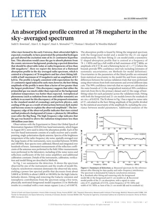
  • 1. 1 m a r c h 2 0 1 8 | V O L 5 5 5 | N A T U R E | 6 7 Letter doi:10.1038/nature25792 An absorption profile centred at 78 megahertz in the sky-averaged spectrum Judd D. Bowman1 , Alan E. E. Rogers2 , Raul A. Monsalve1,3,4 , Thomas J. Mozdzen1 & Nivedita Mahesh1 After stars formed in the early Universe, their ultraviolet light is expected, eventually, to have penetrated the primordial hydrogen gas and altered the excitation state of its 21-centimetre hyperfine line. This alteration would cause the gas to absorb photons from the cosmic microwave background, producing a spectral distortion that should be observable today at radio frequencies of less than 200 megahertz1 . Here we report the detection of a flattened absorption profile in the sky-averaged radio spectrum, which is centred at a frequency of 78 megahertz and has a best-fitting full- width at half-maximum of 19 megahertz and an amplitude of 0.5 kelvin. The profile is largely consistent with expectations for the 21-centimetre signal induced by early stars; however, the best-fitting amplitude of the profile is more than a factor of two greater than the largest predictions2 . This discrepancy suggests that either the primordial gas was much colder than expected or the background radiation temperature was hotter than expected. Astrophysical phenomena (such as radiation from stars and stellar remnants) are unlikely to account for this discrepancy; of the proposed extensions to the standard model of cosmology and particle physics, only cooling of the gas as a result of interactions between dark matter and baryons seems to explain the observed amplitude3 . The low- frequency edge of the observed profile indicates that stars existed and had produced a background of Lyman-α photons by 180 million years after the Big Bang. The high-frequency edge indicates that the gas was heated to above the radiation temperature less than 100 million years later. Observations with the Experiment to Detect the Global Epoch of Reionization Signature (EDGES) low-band instruments, which began in August 2015, were used to detect the absorption profile. Each of the two low-band instruments consists of a radio receiver and a zenith-­ pointing, single-polarization dipole antenna. Spectra of the brightness temperature of the radio-frequency sky noise, spatially averaged over the large beams of the instruments, were recorded between 50 MHz and 100 MHz. Raw spectra were calibrated, filtered and integrated over ­hundreds of hours. Automated measurements of the reflection coeffi- cients of the antennas were performed in the field. Other measurements were performed in the laboratory, including of the noise waves and reflection coefficients of the low-noise amplifiers and additional calibration constants. Details of the instruments, calibration, verifica- tion and model fitting are described in Methods. In Fig. 1 we summarize the detection. It shows the spectrum observed by one of the instruments and the results of model fits. Galactic synchrotron emission dominates the observed sky noise, ­yielding a power-law spectral profile that decreases from about 5,000 K at 50 MHz to about 1,000 K at 100 MHz for the high Galactic latitudes shown. Fitting and removing the Galactic emission and ionospheric contributions from the spectrum using a five-term, physically motivated foreground model (equation (1) in Methods) results in a residual with a root-mean-square (r.m.s.) of 0.087 K. The absorption profile is found by fitting the integrated spectrum with the foreground model and a model for the 21-cm signal simultaneously. The best-fitting 21-cm model yields a symmetric U-shaped absorption profile that is centred at a frequency of 78 ±​ 1 MHz and has a full-width at half-­maximum of − + 19 MHz2 4 , an amplitude of . − . + . 0 5 K0 2 0 5 and a flattening factor of τ= − + 7 3 5 (where the bounds provide 99% confidence intervals including estimates of systematic uncertainties; see Methods for model definition). Uncertainties in the parameters of the fitted profile are estimated from statistical uncertainty in the model fits and from ­systematic differences between the various validation trials that were performed using observations from both instruments and several ­different data cuts. The 99% confidence intervals that we report are calculated as the outer bounds of (1) the marginalized statistical 99% confidence intervals from fits to the primary dataset and (2) the range of best- fitting values for each parameter across the validation trials. Fitting with both the foreground and 21-cm models lowers the residuals to an r.m.s. of 0.025 K. The fit shown in Fig. 1 has a signal-to-noise ratio of 37, calculated as the best-fitting amplitude of the profile divided by the statistical uncertainty of the amplitude fit, including the cova­ riance between model parameters. Additional analyses of the 1 School of Earth and Space Exploration, Arizona State University, Tempe, Arizona 85287, USA. 2 Haystack Observatory, Massachusetts Institute of Technology, Westford, Massachusetts 01886, USA. 3 Center for Astrophysics and Space Astronomy, University of Colorado, Boulder, Colorado 80309, USA. 4 Facultad de Ingeniería, Universidad Católica de la Santísima Concepción, Alonso de Ribera 2850, Concepción, Chile. 1,000 3,000 5,000 Temperature,T(K) a 50 60 70 80 90 100 –0.2 0 0.2 Temperature,T(K) b r.m.s. = 0.087 K c r.m.s. = 0.025 K 50 60 70 80 90 10050 60 70 80 90 100 –0.6 –0.4 –0.2 0 d Temperature,T(K) 50 60 70 80 90 10050 60 70 80 90 100 Frequency, (MHz)Frequency, (MHz) e Figure 1 | Summary of detection. a, Measured spectrum for the reference dataset after filtering for data quality and radio-frequency interference. The spectrum is dominated by Galactic synchrotron emission. b, c, Residuals after fitting and removing only the foreground model (b) or the foreground and 21-cm models (c). d, Recovered model profile of the 21-cm absorption, with a signal-to-noise ratio of 37, amplitude of 0.53 K, centre frequency of 78.1 MHz and width of 18.7 MHz. e, Sum of the 21-cm model (d) and its residuals (c). © 2018 Macmillan Publishers Limited, part of Springer Nature. All rights reserved.
  • 2. 6 8 | N A T U R E | V O L 5 5 5 | 1 m a r c h 2 0 1 8 LetterRESEARCH observations using restricted spectral bands yield nearly identical best-fitting absorption profiles, with the highest signal-to-noise ratio reaching 52. In Fig. 2 we show representative cases of these fits. We performed numerous hardware and processing tests to validate the detection. The 21-cm absorption profile is observed in data that span nearly two years and can be extracted at all local solar times and at all local sidereal times. It is detected by two identically designed instruments operated at the same site and located 150 m apart, and even after several hardware modifications to the instruments, includ- ing orthogonal orientations of one of the antennas. Similar results for the absorption profile are obtained by using two independent pro- cessing pipelines, which we tested using simulated data. The profile is detected using data processed via two different calibration techniques: absolute calibration and an additional differencing-based post- calibration process that reduces some possible instrumental errors. It is also detected using several sets of calibration solutions derived from ­multiple laboratory measurements of the receivers and using ­multiple on-site measurements of the reflection coefficients of the antennas. We modelled the sensitivity of the detection to several possible calibration errors and in all cases recovered profile amplitudes that are within the reported confidence range, as summarized in Table 1. An EDGES high-band instrument operates between 90 MHz and 200 MHz at the same site using a nearly identical receiver and a scaled version of the low-band antennas. It does not produce a similar ­feature at the scaled frequencies4 . Analysis of radio-frequency interference in the observations, including in the FM radio band, shows that the absorption profile is inconsistent with typical spectral contribu- tions from these sources. We are not aware of any alternative astronomical or atmospheric mechanisms that are capable of producing the observed profile. H ii regions in the Galaxy have increasing optical depth with wavelength, blocking more background emission at lower frequencies, but they are observed primarily along the Galactic plane and generate mono- tonic spectral profiles at the observed frequencies. Radio-frequency recombination lines in the Galactic plane create a ‘picket fence’ of narrow absorption lines separated by approximately 0.5 MHz at the observed frequencies5 , but these lines are easy to identify and filter in the EDGES observations. The Earth’s ionosphere weakly absorbs radio signals at the observed frequencies and emits thermal radiation from hot electrons, but models and observations imply a broadband effect that varies depending on the ionospheric conditions6,7 , including diurnal changes in the total electron content. This effect is fitted by our foreground model. Molecules of the hydroxyl radical and nitric oxide have spectral lines in the observed band and are present in the atmosphere, but the densities and line strengths are too low to produce substantial absorption. The 21-cm line has a rest-frame frequency of 1,420 MHz. Expansion of the Universe redshifts the line to the observed band according to ν =​ 1,420/(1 +​ z) MHz, where z is the redshift, which maps uniquely to the age of the Universe. The observed absorption profile is the con- tinuous superposition of lines from gas across the observed redshift range and cosmological volume; hence, the shape of the profile traces the history of the gas across cosmic time and is not the result of the properties of an individual cloud. The observed absorption profile is centred at z ≈​ 17 and spans approximately 20 >​ z >​ 15. The intensity of the observable 21-cm signal from the early Universe is given as a brightness temperature relative to the micro- wave background8 : Ω Ω ≈ . ×        .       +           .        −     T z x z z h T z T z ( ) 0 023 K ( ) 0 15 1 10 0 02 1 ( ) ( ) 21 H m 1 2 b R S I where xHi is the fraction of neutral hydrogen, Ωm and Ωb are the matter and baryon densities, respectively, in units of the critical density for a flat universe, h is the Hubble constant in units of 100 km s−1  Mpc−1 , TR is the temperature of the background radiation, usually assumed to be from the background produced by the afterglow of the Big Bang, TS is the 21-cm spin temperature that defines the relative population of the hyperfine energy levels, and the factor of 0.023 K comes from atomic-line physics and the average gas density. The spin temperature is affected by the absorption of microwave photons, which couples TS to TR, as well as by resonant scattering of Lyman-α​photons and atomic collisions, both of which couple TS to the kinetic temperature of the gas TG. The temperatures of the gas and the background radiation are ­coupled in the early Universe through Compton scattering. This ­coupling becomes ineffective in numerical models9,10 at z ≈​ 150, after which primordial gas cools adiabatically. In the absence of stars or non-standard physics, the gas temperature is expected to be 9.3 K at z =​ 20, falling to 5.4 K at z =​ 15. The radiation temperature decreases more slowly owing to cosmological expansion, following T0(1 + z) with T0 =​ 2.725, and so is 57.2 K and 43.6 K at the same redshifts, ­respectively. The spin temperature is initially coupled to the gas temperature as the gas cools below the radiation temperature, but eventually the decreasing density of the gas is insufficient to main- tain this coupling and the spin temperature returns to the radiation temperature. Redshift, z 14161820222426 Brightnesstemperature,T21(K) –0.6 –0.4 –0.2 0 0.2 H1 H2 H3 H4 H5 H6 P8 Age of the Universe (Myr) 300250200150 Figure 2 | Best-fitting 21-cm absorption profiles for each hardware case. Each profile for the brightness temperature T21 is added to its residuals and plotted against the redshift z and the corresponding age of the Universe. The thick black line is the model fit for the hardware and analysis configuration with the highest signal-to-noise ratio (equal to 52; H2; see Methods), processed using 60–99 MHz and a four-term polynomial (see equation (2) in Methods) for the foreground model. The thin solid lines are the best fits from each of the other hardware configurations (H1, H3–H6). The dash-dotted line (P8), which extends to z >​ 26, is reproduced from Fig. 1e and uses the same data as for the thick black line (H2), but a different foreground model and the full frequency band. Table 1 | Sensitivity to possible calibration errors Error source Estimated uncertainty Modelled error level Recovered amplitude (K) LNA S11 magnitude 0.1 dB 1.0 dB 0.51 LNA S11 phase (delay) 20 ps 100 ps 0.48 Antenna S11 magnitude 0.02 dB 0.2 dB 0.50 Antenna S11 phase (delay) 20 ps 100 ps 0.48 No loss correction N/A N/A 0.51 No beam correction N/A N/A 0.48 The estimated uncertainty for each case is based on empirical values from laboratory ­measurements and repeatability tests. Modelled error levels were chosen conservatively to be five and ten times larger than the estimated uncertainties for the phases and magnitudes, ­respectively. LNA, low-noise amplifier; S11, input reflection coefficient; N/A, not applicable. © 2018 Macmillan Publishers Limited, part of Springer Nature. All rights reserved.
  • 3. 1 m a r c h 2 0 1 8 | V O L 5 5 5 | N A T U R E | 6 9 Letter RESEARCH Over time, Lyman-α​photons from early stars recouple the spin and gas temperatures11 , leading to the detected signal. The onset of the observed absorption profile at z =​ 20 places this epoch at an age of 180 million years, using the Planck 2015 cosmological parameters12 . For the most extreme case, in which TS is fully coupled to TG, the gas and radiation temperatures calculated here yield a maximum absorp- tion amplitude of 0.20 K at z =​ 20, which increases to 0.23 K at z =​ 15. The presence of stars should eventually halt the cooling of the gas and ultimately heat it, because stellar radiation deposits energy into the gas and Lyman-line cooling has been modelled to be very small for the expected stellar properties13 . As early stars die, they are expected to leave behind stellar remnants, such as black holes and neutron stars. The accretion disks around these remnants should generate X-rays, further heating the gas. At some point, the gas is expected to become hotter than the background radiation temperature, ending the absorp- tion signal. The z =​ 15 edge of the observed profile places this transition around 270 million years after the Big Bang. The ages derived for the events above fall within the range expected from many theoretical models2 . However, the flattened shape of the observed absorption profile is uncommon in existing models, and could indicate that the initial flux of Lyman-α​radiation from early stars was sufficiently large that the spin temperature saturated quickly to the gas temperature. We analysed models that assume a high Lyman-α​ flux at z <​ 14 using the EDGES high-band measurements and found a large fraction to be inconsistent with the data4 . To produce the best-fitting profile amplitude of 0.5 K, the ratio TR/TS at the centre of the profile must be larger than 15, compared to a ­maximum of 7 allowed by the gas and radiation temperatures stated above. Even the lower confidence bound of 0.3 K for the observed ­profile amplitude is roughly 50% larger than the strongest predicted signal. For a standard gas temperature history, TR would need to be more than 104 K to yield the best-fitting amplitude at the centre of the profile, whereas for a radiation temperature history given solely by the microwave background, TG would need to be less than 3.2 K. The observed profile amplitude could be explained if the gas and background radiation temperatures decoupled by z ≈​ 250 rather than z ≈​ 150, allowing the gas to begin cooling adiabatically earlier. A ­residual ionization fraction after the formation of atoms that is less than the expected fraction by nearly an order of magnitude would lead to sufficiently early decoupling. However, cross-validation between numerical models and their consistency with Planck observations ­suggest that the residual ionization fraction is already known to approxi­mately 1% fractional accuracy. Considering more exotic scenarios, interactions between dark matter and baryons can explain the observed profile amplitude (by lowering the gas temperature14 ) if the mass of dark-matter particles is below a few gigaelectronvolts and the interaction cross-section is greater than about 10−21  cm2 (ref. 3). Existing models of other non-standard physics, including dark-matter decay and annihilation15 , accreting or evapo- rating primordial black holes16 , and primordial magnetic fields17 , all predict increased gas temperatures and are unlikely to account for the observed amplitude. It is possible that some of these sources could also increase TR through mechanisms such as synchrotron emission associ- ated with primordial black holes18 or the relativistic electrons that result from the decay of metastable particles19 , but it is unclear whether this could compensate for the increased gas temperature. Measurements from ARCADE-2 (ref. 20) suggest an isotropic radio background that cannot be explained by known source populations, but this interpre- tation is still debated21 and the unknown sources would need to be present at z ≈​ 20 to affect the radiation environment relevant to the observed signal. Although we have performed many tests to be confident that the observed profile is from a global absorption of the microwave back- ground by hydrogen gas in the early Universe, we still seek confirma- tion observations from other instruments. Several experiments similar to EDGES are underway. Those closest to achieving the performance required to verify the profile include the Large-Aperture Experiment to Detect the Dark Ages (LEDA)22 , the Sonda Cosmológica de las Islas para la Detección de Hidrógeno Neutro (SCI-HI)23 , the Probing Radio Intensity at high z from Marion (PRIZM) and the Shaped Antenna measurement of the background Radio Spectrum 2 (SARAS 2)24 . The use of more sophisticated foreground models than we have used could lower the performance requirements of the hardware, and could lead to better profile recovery because low-order (smooth) modes in any fitted profile shape tend to be covariant with our foreground model and so are potentially under-constrained. Singular-value decomposition of training sets constructed from simulated instrument error terms and foreground contributions can produce optimized basis sets for model fitting25,26 . We plan to apply these techniques to our data ­processing. The best measurement of the observed profile might ultimately be conducted in space, where the Earth’s atmosphere and ionosphere ­cannot influence the propagation of the astronomical signal, poten- tially reducing the burden of the foreground model. The measurement could be made from the lunar farside27 —either on the surface or from an orbit around the Moon—using the Moon as a shield to block FM radio ­signals and other Earth-based transmitters. This result should bolster ongoing efforts to detect the statistical properties of spatial fluctuations in the 21-cm signal using inter- ferometric arrays; it provides direct evidence that a signal exists for these telescopes to detect. The Hydrogen Epoch of Reionization Array28 (HERA) will become operational over the next two years and will be able to characterize the power spectrum of redshifted 21-cm fluctuations between 100 MHz and 200 MHz during the epoch of reion- ization, when the 21-cm signal should be visible as emission above the background. The operational band of HERA is also expected to be extended to 50 MHz over this time. HERA will probably have suffi- cient thermal sensitivity to detect any power-spectrum signal associ- ated with the EDGES observed profile and so might be able to validate the absorption signal reported here. But foregrounds have proven to be more challenging for interferometers than expected, and sufficient foreground mitigation to detect the 21-cm power spectrum has yet to be demonstrated by any of the currently operating arrays, including the Low-Frequency Array (LOFAR)29 and the Murchison Widefield Array (MWA)30 . Expansion of an ­existing Long Wavelength Array31 station would provide the sensitivity necessary to pursue power- spectrum detection. When constructed, the Square Kilometre Array (SKA) Low-Frequency Aperture Array (https://www.skatelescope.org) should be able to detect the power spectrum associated with the absorp- tion profile reported here and, eventually, to image the 21-cm signal. Online Content Methods, along with any additional Extended Data display items and Source Data, are available in the online version of the paper; references unique to these sections appear only in the online paper. received 13 September 2017; accepted 24 January 2018. 1. Pritchard, J. R. & Loeb, A. 21 cm cosmology in the 21st century. Rep. Prog. Phys. 75, 086901 (2012). 2. Cohen, A., Fialkov, A., Barkana, R. & Lotem, M. Charting the parameter space of the global 21-cm signal. Mon. Not. R. Astron. Soc. 472, 1915–1931 (2017). 3. Barkana, R. Possible interaction between baryons and dark-matter particles revealed by the first stars. Nature 555, https://doi.org/10.1038/nature25791 (2018). 4. Monsalve, R. A., Rogers, A. E. E., Bowman, J. D. & Mozdzen, T. J. Results from EDGES high-band. I. Constraints on phenomenological models for the global 21 cm signal. Astrophys. J. 847, 64 (2017). 5. Alves, M. I. R. et al. The HIPASS survey of the Galactic plane in radio recombination lines. Mon. Not. R. Astron. Soc. 450, 2025–2042 (2015). 6. Rogers, A. E. E., Bowman, J. D., Vierinen, J., Monsalve, R. A. & Mozdzen, T. Radiometric measurements of electron temperature and opacity of ionospheric perturbations. Radio Sci. 50, 130–137 (2015). 7. Sokolowski, M. et al. The impact of the ionosphere on ground-based detection of the global epoch of reionization signal. Astrophys. J. 813, 18 (2015). 8. Zaldarriaga, M., Furlanetto, S. R. & Hernquist, L. 21 centimeter fluctuations from cosmic gas at high redshifts. Astrophys. J. 608, 622–635 (2004). 9. Ali-Haïmoud, Y. & Hirata, C. M. HyRec: a fast and highly accurate primordial hydrogen and helium recombination code. Phys. Rev. D 83, 043513 (2011). © 2018 Macmillan Publishers Limited, part of Springer Nature. All rights reserved.
  • 4. 7 0 | N A T U R E | V O L 5 5 5 | 1 m a r c h 2 0 1 8 LetterRESEARCH 10. Shaw, J. R. & Chluba, J. Precise cosmological parameter estimation using COSMOREC. Mon. Not. R. Astron. Soc. 415, 1343–1354 (2011). 11. Furlanetto, S. R. The global 21-centimeter background from high redshifts. Mon. Not. R. Astron. Soc. 371, 867–878 (2006). 12. Planck Collaboration. Planck 2015 results. XIII. Cosmological parameters. Astron. Astrophys. 594, A13 (2016). 13. Chen, X. & Miralda-Escude, J. The spin-kinetic temperature coupling and the heating rate due to Lyα​scattering before reionization: predictions for 21 centimeter emission and absorption. Astrophys. J. 602, 1–11 (2004). 14. Tashiro, H., Kadota, K. & Silk, J. Effects of dark matter-baryon scattering on redshifted 21 cm signals. Phys. Rev. D 90, 083522 (2014). 15. Lopez-Honorez, L., Mena, O., Moliné, Á., Palomares-Ruiz, S. & Vincent, A. C. The 21 cm signal and the interplay between dark matter annihilations and astrophysical processes. J. Cosmol. Astropart. Phys. 8, 4 (2016). 16. Tashiro, H. & Sugiyama, N. The effect of primordial black holes on 21-cm fluctuations. Mon. Not. R. Astron. Soc. 435, 3001–3008 (2013). 17. Schleicher, D. R. G., Banerjee, R. & Klessen, R. S. Influence of primordial magnetic fields on 21 cm emission. Astrophys. J. 692, 236–245 (2009). 18. Biermann, P. L. et al. Cosmic backgrounds due to the formation of the first generation of supermassive black holes. Mon. Not. R. Astron. Soc. 441, 1147–1156 (2014). 19. Cline, J. M. & Vincent, A. C. Cosmological origin of anomalous radio background. J. Cosmol. Astropart. Phys. 2, 11 (2013). 20. Seiffert, M. et al. Interpretation of the Arcade 2 absolute sky brightness measurement. Astrophys. J. 734, 6 (2011). 21. Vernstrom, T., Norris, R. P., Scott, D. & Wall, J. V. The deep diffuse extragalactic radio sky at 1.75 GHz. Mon. Not. R. Astron. Soc. 447, 2243–2260 (2015). 22. Bernardi, G. et al. Bayesian constraints on the global 21-cm signal from the cosmic dawn. Mon. Not. R. Astron. Soc. 461, 2847–2855 (2016). 23. Voytek, T. C., Natarajan, A., Jáuregui García, J. M., Peterson, J. B. & López-Cruz, O. Probing the dark ages at z ~​20: the SCI-HI 21 cm all-sky spectrum experiment. Astrophys. J. 782, L9 (2014). 24. Singh, S. et al. First results on the epoch of reionization from first light with SARAS 2. Astrophys. J. 845, L12 (2017). 25. Switzer, E. R. & Liu, A. Erasing the variable: empirical foreground discovery for global 21 cm spectrum experiments. Astrophys. J. 793, 102 (2014). 26. Vedantham, H. K. et al. Chromatic effects in the 21 cm global signal from the cosmic dawn. Mon. Not. R. Astron. Soc. 437, 1056–1069 (2014). Acknowledgements We thank CSIRO for providing site infrastructure and access to facilities. We thank the MRO Support Facility team, especially M. Reay, L. Puls, J. Morris, S. Jackson, B. Hiscock and K. Ferguson. We thank C. Bowman, D. Cele, C. Eckert, L. Johnson, M. Goodrich, H. Mani, J. Traffie and K. Wilson for instrument contributions. We thank R. Barkana for theory contributions and G. Holder, T. Vachaspati, C. Hirata and J. Chluba for exchanges. We thank C. Lonsdale, H. Johnson, J. Hewitt and J. Burns. We thank C. Halleen and M. Halleen for site and logistical support. This work was supported by the NSF through awards AST-0905990, AST-1207761 and AST-1609450. R.A.M. acknowledges support from the NASA Ames Research Center (NNX16AF59G) and the NASA Solar System Exploration Research Virtual Institute (80ARC017M0006). This work makes use of the Murchison Radio-astronomy Observatory. We acknowledge the Wajarri Yamatji people as the traditional owners of the site of the observatory. Author Contributions J.D.B., R.A.M. and A.E.E.R. contributed to all activities. N.M. and T.J.M. modelled instrument properties, performed laboratory calibrations and contributed to the preparation of the manuscript. Author Information Reprints and permissions information is available at www.nature.com/reprints. The authors declare no competing financial interests. Readers are welcome to comment on the online version of the paper. Publisher’s note: Springer Nature remains neutral with regard to jurisdictional claims in published maps and institutional affiliations. Correspondence and requests for materials should be addressed to J.D.B. (judd.bowman@asu.edu). Reviewer Information Nature thanks S. Weinreb and the other anonymous reviewer(s) for their contribution to the peer review of this work. 27. Burns, J. O. et al. A space-based observational strategy for characterizing the first stars and galaxies using the redshifted 21 cm global spectrum. Astrophys. J. 844, 33 (2017). 28. DeBoer, D. R. et al. Hydrogen Epoch of Reionization Array (HERA). Publ. Astron. Soc. Pac. 129, 045001 (2017). 29. Patil, A. H. et al. Upper limits on the 21 cm epoch of reionization power spectrum from one night with LOFAR. Astrophys. J. 838, 65 (2017). 30. Beardsley, A. P. et al. First season MWA EoR power spectrum results at redshift 7. Astrophys. J. 833, 102 (2016). 31. Dowell, J., Taylor, G. B., Schinzel, F. K., Kassim, N. E. & Stovall, K. The LWA1 low frequency sky survey. Mon. Not. R. Astron. Soc. 469, 4537–4550 (2017). © 2018 Macmillan Publishers Limited, part of Springer Nature. All rights reserved.
  • 5. Letter RESEARCH Methods Instrument. The EDGES experiment is located at the Murchison Radio-astronomy Observatory (MRO) in Western Australia (26.72° S, 116.61° E), which is the same radio-quiet32 site used by the Australian SKA precursor, the Murchison Widefield Array and the planned SKA Low-Frequency Aperture Array. An early version of EDGES placed an empirical lower limit on the duration of the epoch of reionization33 . EDGES currently consists of three instruments: a high- band instrument4,34,35 that is sensitive to 90–200 MHz (14 >​ z >​ 6) and two low- band instruments (low-1 and low-2) that operate over the range 50–100 MHz (27 >​ z >​ 13). Each instrument yields spectra with 6.1-kHz resolution. In each instrument, sky radiation is collected by a wideband dipole-like antenna that ­consists of two rectangular metal panels mounted horizontally above a metal ground plane. Similar compact dipole antennas are used elsewhere in radio ­astronomy36,37 . A receiver is installed underneath the ground plane and a balun38 is used to guide radiation from the antenna panels to the receiver. A rectangular shroud surrounds the base of the balun to shield the vertical currents in the balun tubes, which are strongest at the base. This lowers the gain towards the horizon owing to the vertical currents. Extended Data Fig. 1 shows a block diagram of the system. A mechanical input switch at the front of the receiver enables the antenna to be connected to a remote vector network analyser (VNA) to measure the antenna reflection coefficients accurately or to be connected to the primary receiver path to measure the sky noise spectrum. When measuring the sky noise spectrum a second ­mechanical switch connects the low-noise amplifier (LNA) to the antenna or to a 26-dB attenuator, which acts as a load or a well matched noise source, depending on the state of the electrical switch on the noise source. This performs a three-position switching operation39 between ambient and ‘hot’ internal noise sources and the antenna, which is needed to provide the first stage of processing discussed below. After the LNA and post-amplifier, another noise source is used to inject noise at less than 45 MHz. This ‘out of band’ conditioning improves the linearity and dynamic range of the analogue-to-digital converter (ADC), which are needed for the ­accurate ­cancellation of the receiver bandpass that is afforded by the three-­ position ­switching. A thermoelectric system maintains a constant temperature in the receiver in the field and in the laboratory. The system mitigates against radio-­frequency interference (RFI) using designs and analysis strategies adapted from the Deuterium Array40 . Similar approaches to instrument design are used for SARAS 2 (ref. 41) and LEDA42 . The design of the low-band instrument differs from the published descriptions of the design of the high-band instrument only by the following. First, a 3-dB attenuator is added within the LNA before the pseudomorphic high-electron- mobility transistor at the input. The attenuator improves the LNA impedance match and thereby reduces the sensitivity to measurement errors of the LNA and antenna reflection coefficients, especially to errors in the reflection phase, while adding only a small amount of noise compared with the sky noise. Larger values of attenuation would begin to add substantial noise at 100 MHz. Second, a scaled antenna is used that is precisely double the size of the antenna of the high-band instrument. Third, a larger ground plane is used. Each ground plane of the low-band instrument consists of a 2 m ×​ 2 m solid metal central assembly surrounded by metal mesh that spans 30 m ×​ 30 m, with the outer 5 m shaped as saw-tooth perforated edges. Low-1 was initially operated with a 10 m ×​ 10 m ground plane and later extended to full size. The full-size 30 m ×​ 30 m ground plane reduces the chromaticity of the beam and makes it less sensitive to con- ditions of the soil. Extended Data Fig. 2 shows the low-1 and low-2 antennas, Extended Data Fig. 3 the measured reflection coefficients and Extended Data Fig. 4 cuts through the model of the antenna beam pattern. Calibration. We implement end-to-end absolute calibration for the low-band instruments following the techniques developed for the high-band instrument34,43 . The calibration procedure involves taking reference spectra in the laboratory with the receiver connected to hot and ambient loads and to open and shorted cables. Similar techniques are used in other microwave measurements44,45 . Reflection coefficient measurements using a VNA are acquired for the calibration sources and the LNA. The input connection to the receiver box provides the reference plane for all VNA measurements. To correct for the losses in the hot load used in the laboratory for calibration, full scattering parameters are measured for the short cable from the heated resistor in the hot load. The accuracy of scattering parameter measurements is improved by accounting for the actual resistance of the 50-Ω​load used for VNA calibration and the added inductance in the load due to skin effects46 in the few millimetres of transmission line between its internal termination and the reference plane47 . The calibration spectra and reflection coefficient measurements acquired in the laboratory are used to solve for the free parameters34 in the equations that account for the impedance mismatches between the receiver and the antenna and for the correlated and uncorrelated LNA noise waves. Laboratory calibration is performed with the receiver temperature controlled to the default 25 °C, and at 15 °C and 35 °C to assess the thermal dependence of the calibration parameters. Extended Data Fig. 5 shows calibration parameter solutions for both receivers. Following calibration in the laboratory, a test is performed by measuring the spectrum of an approximately 300 K passive load with deliberate impedance ­mismatch that approximately mimics the reflection from the antenna in magnitude and phase. We call this device an ‘artificial antenna simulator’. The reflection coefficient of the antenna simulator is measured and applied to yield calibrated integrated spectra. Extended Data Fig. 3 shows measured reflection coefficients for the artificial antenna simulator. Once corrected, the integrated spectra are expected to be spectrally flat, with a noise temperature that matches the physical temperature of the passive load. The flatness of an integrated spectrum is quantified through the r.m.s. of the residuals after subtracting a constant term. The typical r.m.s. of the ­residuals is 0.025 K over the range 50–100 MHz. If a three-term polynomial (equation (2) with N =​ 3) is subtracted, then the residuals decrease to about 0.015 K and are limited by integration time. A second test of the calibration is performed by measuring the spectrum of a noise source followed by a filter and an approximately 3-m cable that adds about 30 ns of two-way delay. The device yields a spectrum that is similar in shape to the sky foreground with a strength of about 10,000 K (seven times larger than the ­typical sky temperature observed by EDGES) at 75 MHz and has a reflection coefficient of −​6 dB in magnitude with a phase slope similar to that of the antenna. Typical residuals are less than 300 mK after subtracting a five-term polynomial (equation (2)) and are limited by integration time. Assuming any residuals scale with input power, this value corresponds to residuals of 45 mK at the typical observed sky temperature. This test is more sensitive than the passive ­simulator, especially to errors in the measurements of the reflection coefficient, because the signal is 33 times stronger than that of the approximately 300-K load and because the magnitude of the reflection of this simulator is larger than that of the passive simulator and of the real antenna. Losses in the balun and losses due to the finite ground plane are corrected for during data processing using models. The balun-loss model is validated against scattering parameter measurements. Frequency-dependent beam effects are com- pensated for by modelling and subtracting the spectral structure using electro­ magnetic beam models and a diffuse sky map template35 . The nominal beam model accounts for the finite metal ground plane over soil with a relative permittivity of 3.5 and conductivity of 2 ×​ 10−2  S m−1 (ref. 48). The sky template is produced by extrapolating the 408-MHz all-sky radio map49 to the observed frequencies using a spectral index in brightness temperature of −​2.5 (refs 35, 43). Data and processing. Examples of raw and processed data are shown in Extended Data Fig. 6. Data processing involves three primary stages. In the first stage, three raw spectra that have each been accumulated for 13 s from the antenna input and two internal reference noise sources are converted into a single ­partially ­calibrated spectrum39 . Individual 6.1-kHz channels above a fixed power threshold are assigned zero weight to remove RFI. The threshold is normally set at three times the r.m.s. of the residuals after substacting a constant and a slope in a ­sliding 256-spectral-channel window. Similarly, any partially calibrated spectrum with an ­average power above that expected from the sky or with large residuals is ­discarded. A weighted average of many successive spectra is taken, typically over several hours. Outlier channels after a Fourier series fit to the entire accumulated spectrum are again assigned zero weight. This second pass assigns zero weight to lower levels of RFI and broader RFI signals than does the initial pass. Inthesecondstageofprocessing,thepartiallycalibratedspectraarefullycalibrated usingthecalibrationparametersfromthelaboratoryandtheantennareflectioncoef- ficient measurements taken periodically in the field. Beam-chromaticity corrections areappliedafteraveragingthemodeloverthesamerangeoflocalsiderealtimesasfor the spectra. The spectra are then corrected for the balun and ground-plane loss and output with a typical smoothing to spectral bins with 390.6-kHz resolution. In the third stage of processing, spectra for each block of local sidereal time of several hours within each day are fitted with a foreground model (see below for description of models). An r.m.s. value of the residuals is computed for each block and blocks above a selected threshold are discarded, typically because of broad- band RFI—or solar activity in daytime data—that was not detected in the earlier processing stages. A weighted average is then taken of the accepted blocks and a weighted least-squares solution is determined using a foreground model along with the model that represents the 21-cm absorption signal. Extended Data Fig. 7 shows the final weights for each spectral bin, equivalent to the RFI occupancy. The observations used for the primary analysis presented here are from low-1, spanning 2016 day 252 through to 2017 day 94 (configuration H2 below). The data are filtered to retain only local Galactic hour angles (GHA) of 6–18 h; GHA is equivalent to the local sidereal time offset by 17.75 h. © 2018 Macmillan Publishers Limited, part of Springer Nature. All rights reserved.
  • 6. LetterRESEARCH Parameter estimation. The polynomial foreground model used for the analysis presented in Fig. 1 is physically motivated, with five terms based on the known spectral properties of the Galactic synchrotron spectrum and Earth’s ionosphere6,50 : ν ν ν ν ν ν ν ν ν ν ν ν ν ν ν ≈       +             +                     +       +       − . − . − . − . − T a a a a a ( ) log log (1) F 0 c 2 5 1 c 2 5 c 2 c 2 5 c 2 3 c 4 5 4 c 2 where TF(ν) is the brightness temperature of the foreground emission, ν is ­the frequency, νc is the centre frequency of the observed band and the coefficients an are fitted to the data. The above function is a linear approximation, centred on νc, to ν ν ν ν ν =       +       ν ν ν ν − . + + / − / − − T b b( ) e b b b F 0 c 2 5 log( ) ( ) 4 c 21 2 c 3 c 2 which is connected directly to the physics of the foreground and the ionosphere. The factor of −​2.5 in the first exponent is the typical power-law spectral index of the foreground, b0 is an overall foreground scale factor, b1 allows for a correction to the typical spectral index of the foreground (which varies by roughly 0.1 across the sky) and b2 captures any contributions from a higher-order foreground spectral term51,52 . Ionospheric contributions are contained in b3 and b4, which allow for the ionospheric absorption of the foreground and emission from hot electrons in the ionosphere, respectively. This model can also partially capture some instrumental effects, such as additional spectral structure from chromatic beams or small errors in calibration. We also use a more general polynomial model in many of our trials that enables us to explore signal recovery with varying numbers of polynomial terms: ∑ν ν= = − − .T a( ) (2) n N n n F 0 1 2 5 where N is the number of terms and the coefficients an are again fitted to the data. As with the physical model, the −​2.5 in the exponent makes it easier for the model to match the foreground spectrum. Both foreground models yield consistent absorption profile results. The 21-cm absorption profile is modelled as a flattened Gaussian: ν = −    − −    τ τ − − T A( ) 1 e 1 e 21 eB where ν ν τ = −     −    +        τ− B w 4( ) log 1 log 1 e 2 0 2 2 and A is the absorption amplitude, ν0 is the centre frequency, w is the full-width at half-maximum and τ is a flattening factor. This model is not a description of the physics that creates the 21-cm absorption profile, but rather is a suitable functional form to capture the basic shape of the profile. Extended Data Fig. 8 shows the best-fitting profile and residuals from fits by the two foreground models. We report parameter fits from a gridded search over the parameters ν0, w and τ in the 21-cm model. For each step in the grid, we conduct a linear weighted least-squares fit, solving simultaneously for the foreground coefficients and the amplitude of the absorption profile. The best-fitting absorption profile maximizes the signal-to-noise ratio in the gridded search. The uncertainty in the amplitude fit accounts for covariance between the foreground coefficients and the amplitude of the profile and for noise. Fitting both foreground and 21-cm models simultaneously yields residuals that decrease with integration time with an approximately noise-like ( / t1 ) trend for the duration of the observation, whereas fitting only the foreground model yields residuals that decrease with time for the first approximately 10% of the integration and then saturate, as shown in Extended Data Fig. 9. We also performed a Markov chain Monte Carlo (MCMC) analysis (Extended Data Fig. 10) for the H2 case using a five-term polynomial (equation (2)) for the foreground model and a subset of the band covering 60–94 MHz. The amplitude parameter is most covariant with the flattening. The 99% statistical confidence intervals on the four 21-cm model parameters are: = . − . + . A 0 52 K0 18 0 42 , ν = . − . + . 78 3 MHz0 0 3 0 2 , = . − . + . w 20 7 MHz0 7 0 8 and τ = . − . + . 6 5 2 5 5 6 . These intervals do not include any systematic error from differences across the hardware configurations and processing trials. When the flattening parameter is fixed to τ =​ 7, statistical uncertainty in the 21-cm model amplitude fit is reduced to approximately ±​0.02 K. Extended Data Table 1 shows that the various hardware configurations and ­processing trials with fixed τ =​ 7 yield best-fitting parameter ranges of 0.37 K <​ A <​ 0.67 K, 77.4 MHz <​ ν0 <​ 78.5 MHz and 17.0 MHz <​ w <​ 22.8 MHz. This systematic variation is probably due to the limited data in the some of the configurations, small calibration errors and residual chromatic beam effects, and potentially to structure in the Galactic foreground that increases when the Galactic plane is overhead. For each parameter, taking the outer bounds of the statistical confidence ranges from the comprehensive MCMC analysis for H2 and the best-­ fitting variations between validation trials in Extended Data Table 1 yields the estimate of the 99% confidence intervals that we report in the main text. Verification tests. Here we list the tests that we performed to verify the ­detection. The absorption profile is detected from data obtained in the following hard- ware configurations: H1, low-1 with 10 m ×​ 10 m ground plane; H2, low-1 with 30 m ×​ 30 m ground plane; H3, low-1 with 30 m ×​ 30 m ground plane and ­recalibrated receiver; H4, low-2 with north–south dipole orientation; H5, low-2 with east–west dipole orientation; and H6, low-2 with east–west dipole orientation and the balun shield removed to check for any resonance that might result from a slot antenna being formed in the joint between the two halves of the shield. The absorption profile is detected in data processed with the following ­configurations: P1, all hardware cases, using two independent processing ­pipelines; P2, all hardware cases, divided into temporal subsets; P3, all hardware cases, with chromatic beam corrections on or off; P4, all hardware cases, with ground loss and balun loss corrections on or off; P5, all hardware cases, calibrated with four different antenna reflection coefficient measurements; P6, all hardware cases, using a four-term foreground model (equation (2)) over the frequency range 60–99 MHz; P7, all hardware cases, using a five-term foreground model (equation (2)) over the frequency range 60–99 MHz; P8, all hardware cases, using the physical foreground model (equation (1)) over the frequency range 51–99 MHz; P9, all hardware con- figurations, using various additional combinations of four-, five-, and six-term foreground models (equation (2)) and various frequency ranges; P10, H2 binned by local sidereal time/GHA; P11, H2 binned by utc; P12, H2 binned by buried conduit temperature as a proxy for the ambient temperature at the receiver and the temperature of the cable that connects the receiver frontend under the antenna to the backend in the control hut; P13, H2 binned by Sun above or below the ­horizon; P14, H2 binned by Moon above or below the horizon; P15, H2 with added post-calibration calculated by subtracting scaled Galaxy-up spectra from Galaxy-down spectra; P16, H2 calibrated with low-2 solutions; P17, H4 calibrated with laboratory measurements at 15 °C and 35 °C; and P18, H2 and H3 calibrated with laboratory measurements spanning two years. Extended Data Table 1 lists the properties of the profile for each of the hardware configurations (H1–H6) with the standard processing configuration (P6); Fig. 2 illustrates the corresponding best-fitting profiles. The variations in signal-to- noise ratio between the configurations are largely explained by differences in the total integration time for each configuration, except for H1, which was limited by its ground-plane performance. We acquired the most data in configura- tion H1, with approximately 11 months of observations, followed by H2 with 6 months. The other configurations were each operated for 1–2 months before the analysis ­presented here was performed. Extended Data Table 2 lists the profile amplitudes for data binned by GHA for both processing pipelines used in configuration P1. The following additional verification tests were performed to check specific aspects of the instrument, laboratory calibration and processing pipelines. (1) We processed simulated data and recovered injected profiles. (2) We searched for a similar profile at the scaled frequencies in high-band data and found no corre- sponding profile. (3) We measured the antenna reflection coefficients of low-2 with the VNA connected to its receiver via a short 2-m cable and found nearly identical results to when the 100-m cable was used (under normal operation). (4) We acquired in situ reflection coefficient measurements that matched our model predictions of the low-2 balun with the antenna terminal shorted and open; this was done to verify our model for the balun loss. (5) We tested the performance of the receivers in the laboratory using artificial antenna sources connected to the receivers directly, as described above. (6) We cross-checked our beam models using three electromagnetic numerical solvers: CST, FEKO and HFSS. Although no beam model is required to detect the profile because the EDGES antenna is designed to be largely achromatic, we performed the cross-check because we apply beam corrections in the primary analysis. Sensitivity to systematic errors. Here we discuss in more detail several primary categories of potential systematic errors and the validation steps that we performed. Beam and sky effects. Beam chromaticity is larger than can be accounted for with electromagnetic models of the antenna on an infinite ground plane53 . For both ground plane sizes, the r.m.s. of the residuals to low-order foreground polynomial model fits of the data matched electromagnetic modelling when the model accounted for the finite ground-plane size and included the effects of the ­dielectric © 2018 Macmillan Publishers Limited, part of Springer Nature. All rights reserved.
  • 7. Letter RESEARCH constant and the conductivity of the soil under the ground plane. The residual structures themselves matched qualitatively. Comparing electromagnetic solvers for beam models, we found that for infinite ground-plane models the change in the absolute gain of the beam with frequency at every viewing angle (θ, φ) was within ±​0.006 between solvers and that residuals after foreground fits to simulated spectra were within a factor of two. For models with finite ground planes and real soil properties, we found that correcting H1 data using beam models from FEKO and HFSS in integral solver modes resulted in nearly identical 21-cm model parameter values, although using an HFSS model for the larger ground plane in H2 resulted in a fit to the profile that had a lower signal-to-noise ratio than when using the FEKO model, but still a higher signal-to-noise ratio than when no beam correction was used (see Extended Data Table 1). The low-2 instrument was deployed 100 m west of the control hut, whereas the low-1 instrument was 50 m east of the hut. In the east–west antenna orientation, the low-2 dipole-response null was aimed approximately at the control hut and the beam pattern on the sky was rotated relative to north–south. Obtaining consistent absorption profiles with the two sizes of low-1 ground planes (H1 versus H2 or H3) and with both low-2 antenna orientations (H4 versus H5 or H6) suggests that beam effects are not responsible for the profile, while obtaining the same results from both low-2 antenna orientations also disfavours polarized sky emission as a possible source of the profile. Obtaining consistent absorption profiles with the low-1 and low-2 instruments at different distances from the control hut and with both low-2 antenna orientations suggests that it is unlikely that the observed profile is produced by reflections of sky noise from the control hut or other surrounding objects or caused by RFI from the hut. Our understanding of hut reflections is further validated by the appearance of small sinusoidal ripples after subtracting a nine-term foreground model (equation (2)) from the low-1 spectra at GHA 20. These ripples are consistent with models of hut reflections and not evident at other GHAs or in the low-2 data. Gain and loss errors. Many possible instrumental systematic errors and atmospheric effects that could potentially mimic the observed absorption profile are due to inaccurate or unaccounted for gains or losses in the propagation path within the instrument or Earth’s atmosphere. If present, these effects would be proportional to the total sky noise power entering the system. The total sky noise power received by EDGES varies by a factor of three over GHA. If the observed absorption profile were due to gain or loss errors, the amplitude of the profile would be expected to vary in GHA proportional to the sky noise. We tested for these errors by fitting for the absorption profile in observations binned by GHA in 4-h and 6-h blocks using H2 data. The test is complicated by the increase in chromatic-beam effects in spectra when the sky noise power is large owing to the presence of the Galactic plane in the antenna beam. We compensated for this by increasing the foreground model to up to six polynomial terms for the GHA analysis and using the FEKO antenna beam model to correct for beam effects. As evident in Extended Data Table 2, the best-fitting amplitudes averaged over each GHA bin are consistent within the reported uncertainties and exhibit no substantial correlation with sky noise power. The same test performed using a four-term polynomial foreground model (equation (2)) did yield varia- tions with GHA, as did tests performed on data from low-1 with the 10 m ×​ 10 m ground plane. We attribute the failure of these two cases to beam effects and possible foreground structure. Other cases tested had insufficient data for con- clusive results, but did not show any correlation with the total sky noise power. The artificial antenna measurements described in Methods section ‘Calibration’ provide verification of the smooth passband of the receiver after calibration. Because we observe the 0.5-K signature for all foreground conditions, including low foregrounds of about 1,500 K at about 78 MHz, if the observed profile were an instrumental artefact due to an error in gain of the receiver, then we would expect to see a scaled version of the profile with an amplitude of 0.5 K ×​ (300 K/1,500 K)  =​ 0.1 K when measuring the approximately 300-K artificial antenna. Instead, we see a smooth spectrum structure at the approximately 0.025-K level. With the 10,000-K artificial antenna, we would expect to see a 3.3-K profile that yields 0.5-K residuals after subtracting a five-term polynomial fit (equation (2)); instead we find residuals that are less than 0.3 K. Receiver calibration errors are disfavoured as the source of the observed ­profile. Three verification tests were performed to investigate this possibility specifi- cally by processing data with inaccurate calibration parameter solutions. First, in verification test P18 we processed H2 and H3 datasets using each of the three low-1 receiver calibration solutions shown in Extended Data Fig. 5a–g. The observed pro- file was detected in each case, indicating that the detection is robust to these small drifts in the calibration parameters over the two-year period spanning the use of the low-1 receiver. Second, in verification test P17 we processed H4 observations using the calibration solutions derived from laboratory measurements acquired with the receiver temperature held at both 15 °C and 35 °C, even though it was controlled to 25 °C for all observations. The profile was recovered even for these larger calibration differences and so we infer that the detection is robust to the much smaller variations of typically 0.1 °C in the receiver temperature around its set point during operation. Third, as a final check of the receiver properties, in P16 we calibrated the H2 dataset from low-1 using the receiver calibration ­solutions derived for low-2. The profile was recovered using a seven-term foreground model ­(equation (2)) over the range 53–99 MHz. This provides evidence that both ­receivers have generally similar properties and spectrally smooth responses; otherwise, we would not expect the calibration solutions to be interchangeable in this manner. RFI and FM radio. RFI is found to be minimal in EDGES low-band ­measurements. We rule out locally generated broadband RFI from the control hut and a nearby ASKAP dish (more than 150 m away) as the source of the profile because of the consistent profiles observed by both instruments and both low-2 antenna orientations, as noted above. There are no licensed digital TV transmitters in Australia below 174 MHz (https://www.acma.gov.au, ITU RCC-06). We ­analysed observations and rule out the FM radio band, which spans 87.5–108 MHz, as the cause of the high-frequency edge of the observed profile. FM transmissions within about 3,000 km of the MRO could be scattered from aeroplanes or from ­meteors that burn up at an altitude of about 100 km in the mesosphere. Inspection of ­channels removed by our RFI detection algorithms and of spectral residuals using the instrument’s raw 6.1-kHz resolution, which oversamples the minimum 50-kHz spacing of the FM channel centres, shows that these signals are sparse and transient and show up after removal as mostly zero-weighted channels. More persistent worldwide FM signals reflected from the Moon have been measured54 from the MRO with flux density about 100 Jy. We find evidence for a sharp step of around 0.05 K at 87.5 MHz in our binned spectra when the Moon is above 45° elevation, which can be eliminated by using only data from when the Moon is below the horizon. Atmospheric molecular lines. Atmospheric nitrous oxide line absorption was modelled using a line strength of 10−12.7  nm2  MHz at 300 K based on values from the spectral line catalogue maintained by the Molecular Spectroscopy Team at the Jet Propulsion Laboratory and an abundance of 70 parts per billion. We assumed a 3,000-K sky-noise temperature and a line-of-sight path through the atmosphere at 8° elevation and integrated over the altitude range 10–120 km. We find up to 0.001 mK of absorption per line. With approximately 100 individual lines between 50 MHz and 100 MHz, we conservatively estimate a maximum possible contribu- tion of 0.1 mK. Gas temperature and residual ionization fraction. For the gas thermal calcu- lations, we used CosmoRec10 to model the evolution of the electron temperature and residual ionization fraction for z <​ 3,000. We verified the output against solu- tions to equations55 for the dominant contributions to the electron temperature evolution of adiabatic expansion and Compton scattering. We assume that the gas temperature is in equilibrium with the electron temperature. To determine the residual ionization fraction that is required to produce sufficiently cold gas to account for the observed profile amplitude, we modelled a partial ionization step function in redshift. We used the ionization fraction from CosmoRec for redshifts above the transition and a constant final ionization fraction below the transition. We performed a grid search in transition redshift and final ionization fraction to identify the lowest transition redshift for the largest final ionization fraction that results in the required gas temperature. We found that a final ionization fraction of around 3 ×​ 10−5 reached by z ≈​ 500 would be sufficient to produce the required gas temperature. This is nearly an order of magnitude lower than the expected ionization fraction of around 2 ×​ 10−4 at similar ages from CosmoRec. Data availability. The data that support the findings of this study are available from the corresponding author on reasonable request. Code availability. The code that supports the findings of this study is available from the corresponding author on reasonable request. 32. Bowman, J. & Rogers, A. E. E. VHF-band RFI in geographically remote areas. In Proc. RFI Mitigation Workshop id.30, https://pos.sissa.it/107/030/pdf (Proceedings of Science, 2010). 33. Bowman, J. D. & Rogers, A. E. E. Lower Limit of Δ​z>​0.06 for the duration of the reionization epoch. Nature 468, 796–798 (2010). 34. Monsalve, R. A., Rogers, A. E. E., Bowman, J. D. & Mozdzen, T. J. Calibration of the EDGES high-band receiver to observe the global 21 cm signature from the epoch of reionization. Astrophys. J. 835, 49 (2017). 35. Mozdzen, T. J., Bowman, J. D., Monsalve, R. A. & Rogers, A. E. E. Improved measurement of the spectral index of the diffuse radio background between 90 and 190 MHz. Mon. Not. R. Astron. Soc. 464, 4995–5002 (2017). 36. Raghunathan, A., Shankar, N. U. & Subrahmanyan, R. An octave bandwidth frequency independent dipole antenna. IEEE Trans. Anenn. Propag. 61, 3411–3419 (2013). 37. Ellingson, S. W. Antennas for the next generation of low-frequency radio telescopes. IEEE Trans. Antenn. Propag. 53, 2480–2489 (2005). 38. Roberts, W. K. A new wide-band balun. Proc. IRE 45, 1628–1631 (1957). © 2018 Macmillan Publishers Limited, part of Springer Nature. All rights reserved.
  • 8. LetterRESEARCH 39. Bowman, J. D., Rogers, A. E. E. & Hewitt, J. N. Toward empirical constraints on the global redshifted 21 cm brightness temperature during the epoch of reionization. Astrophys. J. 676, 1–9 (2008). 40. Rogers, A. E. E., Pratap, P., Carter, J. C. & Diaz, M. A. Radio frequency interference shielding and mitigation techniques for a sensitive search for the 327 MHz line of deuterium. Radio Sci. 40, RS5S17 (2005). 41. Singh, S. et al. SARAS 2: a spectral radiometer for probing cosmic dawn and the epoch of reionization through detection of the global 21 cm signal. Preprint at https://arxiv.org/abs/1710.01101 (2017). 42. Price, D. C. et al. Design and characterization of the Large-Aperture Experiment to Detect the Dark Age (LEDA) radiometer systems. Preprint at https://arxiv. org/abs/1709.09313 (2017). 43. Rogers, A. E. E. & Bowman, J. D. Absolute calibration of a wideband antenna and spectrometer for accurate sky noise temperature measurement. Radio Sci. 47, RS0K06 (2012). 44. Hu, R. & Weinreb, S. A novel wide-band noise-parameter measurement. IEEE Trans. Microw. Theory Tech. 52, 1498–1507 (2004). 45. Belostotski, L. A calibration method for RF and microwave noise sources. IEEE Trans. Microw. Theory Tech. 59, 178–187 (2011). 46. Ramo, S. & Whinnery, J. R. Fields and Waves in Modern Radio Ch. 6 (Wiley, 1953). 47. Monsalve, R. A., Rogers, A. E. E., Mozdzen, T. J. & Bowman, J. D. One-port direct/reverse method for characterizing VNA calibration standards. IEEE Trans. Microw. Theory Tech. 64, 2631–2639 (2016). 48. Sutinjo, A. T. et al. Characterization of a low-frequency radio astronomy prototype array in Western Australia. IEEE Trans. Antenn. Propag. 63, 5433–5442 (2015). 49. Haslam, C. G. T., Salter, C. J., Stoffel, H. & Wilson, W. E. A 408 MHz all-sky continuum survey. II. The atlas of contour maps. Astron. Astrophys. Suppl. Ser. 47, 1–143 (1982). 50. Chandrasekhar, S. Radiative Transfer (Courier Dover, 1960). 51. de Oliveira-Costa, A. et al. A model of diffuse Galactic radio emission from 10 MHz to 100 GHz. Mon. Not. R. Astron. Soc. 388, 247–260 (2008). 52. Bernardi, G., McQuinn, M. & Greenhill, L. J. Foreground model and antenna calibration errors in the measurement of the sky-averaged λ​21 cm signal at z ~​ 20. Astrophys. J. 799, 90 (2015). 53. Mozdzen, T. J., Bowman, J. D., Monsalve, R. A. & Rogers, A. E. E. Limits on foreground subtraction from chromatic beam effects in global redshifted 21 cm measurements. Mon. Not. R. Astron. Soc. 455, 3890–3900 (2016). 54. McKinley, B. et al. Low-frequency observations of the Moon with the Murchison widefield array. Astron. J. 145, 23 (2013). 55. Seager, S., Sasselov, D. D. & Scott, D. How exactly did the Universe become neutral? Astrophys. J. Suppl. Ser. 128, 407–430 (2000). © 2018 Macmillan Publishers Limited, part of Springer Nature. All rights reserved.
  • 9. Letter RESEARCH Extended Data Figure 1 | Block diagram of the low-band system. The inset images show: a, the capacitive tuning bar that feeds the dipoles at the top of the balun; b, the SubMiniature version A connector at the bottom of the balun coaxial transmission line where the receiver connects; c, the low-1 receiver that is installed under its antenna with the ground-plane cover plate removed; and d, the inside of the low-1 receiver. The LNA is contained in the secondary metal enclosure in the lower-left corner of the receiver. SW, switch. © 2018 Macmillan Publishers Limited, part of Springer Nature. All rights reserved.
  • 10. LetterRESEARCH Extended Data Figure 2 | Low-band antennas. a, The low-1 antenna with the 30 m ×​ 30 m mesh ground plane. The darker inner square is the original 10 m ×​ 10 m mesh. The control hut is 50 m from the antenna. b, A close view of the low-2 antenna. The two elevated metal panels form the dipole-based antenna and are supported by fibreglass legs. The balun consists of the two vertical brass tubes in the middle of the antenna. The balun shield is the shoebox-sized metal shroud around the bottom of the balun. The receiver is under the white metal platform and is not visible. © 2018 Macmillan Publishers Limited, part of Springer Nature. All rights reserved.
  • 11. Letter RESEARCH Extended Data Figure 3 | Antenna and simulator reflection coefficients. a, b, Measurements of the reflection coefficient magnitude (a) and phase (b) are plotted for hardware configurations H2 (blue), H4 (red) and H6 (yellow). The antennas are designed identically (except H6 has the balun shield removed), but are tuned manually during installation by adjusting the panel separation and the height of the small metal plate that connects one panel to the centre conductor of the balun transmission line on the other. The measurements were acquired in situ. c, d, The red curve is the 10,000-K artificial antenna noise source and the blue curve is the 300-K mismatched load. © 2018 Macmillan Publishers Limited, part of Springer Nature. All rights reserved.
  • 12. LetterRESEARCH Extended Data Figure 4 | Antenna beam model. a, Beam cross-sections showing the gain in the plane containing the electric field (dashed) and in the plane containing the magnetic field (solid) from FEKO for the H2 antenna and ground plane over soil. Cross-sections are plotted at 50 MHz (red), 70 MHz (yellow) and 100 MHz (blue). b, Frequency dependence of the gain at zenith angle Θ =​ 0° (solid) and the 3-dB points at 70 MHz in the electric-field plane (dashed) and magnetic-field plane (dotted). c, Small undulations with frequency, after a five-term polynomial (equation (2)) has been subtracted from each of the curves, are plotted as fractional changes in the gain. Simulated observations with this model yield residuals of 0.015 K (0.001%) to the five-term fit over the frequency range 52–97 MHz at GHA =​ 10 and residuals of 0.1 K (0.002%) at GHA =​ 0, showing that the cumulative beam yields less chromaticity than the approximately 0.5% variations in the individual points plotted. 0 20 40 60 80 [deg] 0 1 2 3 4 5 6 7 Gain[linear] (a) 3 4 5 6 7 Gain[linear] (b) 50 60 70 80 90 100 [MHz] -1 0 1 [%] (c) © 2018 Macmillan Publishers Limited, part of Springer Nature. All rights reserved.
  • 13. Letter RESEARCH Extended Data Figure 5 | Calibration parameter solutions. a–g, Solutions for the low-1 receiver at its fixed 25 °C operating temperature. It was calibrated on three occasions spanning two years, bracketing all of the low-1 observations reported. The first calibration was in August 2015 before commencing cases H1 and H2 (solid), the next was in May 2017 before H3 (dotted), and the final was in September 2017 after the conclusion of H3 (dashed). h–n, Solutions for the low-2 receiver controlled to three different temperatures: 15 °C (blue), 25 °C (black) and 35 °C (red). The parameters C1 and C2 are scale and offset factors, respectively; TC, TS and TU are noise-wave parameters (TS is not the spin temperature here; see ref. 34 for details); S11 is the LNA input reflection coefficient. -40 -30 [dB] (a) S11 mag Low-1 20 40 60 80 100 120 [deg] (b) S11 phase 3 4 5 (c) C1 -10 0 10 T[K] (d) C2 -20 -10 0 10 T[K] (e) TC 0 10 20 30 T[K] (f) TS 50 60 70 80 90 100 [MHz] 180 190 T[K] (g) TU -40 -30 [dB] (h) S11 mag Low-2 20 40 60 80 100 120 [deg] (i) S11 phase 3 4 5 (j) C1 -10 0 10 T[K] (k) C2 -20 -10 0 10 T[K] (l) TC 0 10 20 30 T[K] (m) TS 50 60 70 80 90 100 [MHz] 180 190 T[K] (n) TU © 2018 Macmillan Publishers Limited, part of Springer Nature. All rights reserved.
  • 14. LetterRESEARCH Extended Data Figure 6 | Raw and processed spectra. a, Typical raw 13-s spectra from H2 for each of the receiver’s ‘three position’ switch states. The small spikes on the right of the antenna spectrum are FM radio stations. b, The spectrum has been partially calibrated (‘Three position’) using the three raw spectra to correct gain and offset contributions in the receiver and cables, then fully calibrated (Calib.) by applying the calibration parameter solutions from the laboratory to yield the sky temperature. c, Residuals to a fit of the fully calibrated spectrum with the five-term polynomial foreground model (equation (2)). In b and c, the frequencies listed in the legend give the binning used for each curve. -85 -80 -75 Power[dB] (a) Antenna Internal - Ambient Internal - 'Hot' 0 1000 2000 3000 4000 5000 T[K] (b) 'Three position' Calib. (6.1 kHz) Calib. (390.6 kHz, RFI excised) 50 60 70 80 90 100 [MHz] -50 0 50 T[K] (c) Residual (6.1 kHz) Residual (390.6 kHz) © 2018 Macmillan Publishers Limited, part of Springer Nature. All rights reserved.
  • 15. Letter RESEARCH Extended Data Figure 7 | Normalized channel weights. The fraction of data integrated for each 390.6-kHz spectral bin are shown. a, The FM band causes the low weights above 87 MHz, because many 6.1-kHz raw spectral channels in this region are removed for all times. The weights are nearly identical across all hardware cases (H1–H6). b, A close-up showing the weights below the FM band, where there is little RFI to remove. © 2018 Macmillan Publishers Limited, part of Springer Nature. All rights reserved.
  • 16. LetterRESEARCH Extended Data Figure 8 | Residuals to the 21-cm profile model. The black curve shows the best-fitting 21-cm profile model derived from the observations. The solid blue and yellow curves show fits to the model profile using the physical (equation (1)) and five-term polynomial (equation (2)) foreground models, respectively. The dashed lines show the residuals after subtracting the fits from the model. These residuals are similar to those found when fitting the observations using only a foreground model (Fig. 1b). © 2018 Macmillan Publishers Limited, part of Springer Nature. All rights reserved.
  • 17. Letter RESEARCH Extended Data Figure 9 | Residual r.m.s. as a function of integration time. The curves show the residual r.m.s. after a best-fitting model is removed at each integration time for the H2 dataset. 1 10 100 Integration time [hours] 0.01 0.1 Residualr.m.s.[K] Reference: t-1/2 Foreground model only Foreground and 21-cm models © 2018 Macmillan Publishers Limited, part of Springer Nature. All rights reserved.
  • 18. LetterRESEARCH Extended Data Figure 10 | Parameter estimation. Likelihood distributions for the foreground and 21-cm model parameters are shown for the H2 dataset. Contours are drawn at the 68% and 95% probability levels. The foreground polynomial coefficients (an) are highly correlated with each other, whereas the 21-cm model parameters are largely uncorrelated, except for the profile amplitude (A) and flattening (τ). Systematic uncertainties from the verification hardware cases are not presented here. © 2018 Macmillan Publishers Limited, part of Springer Nature. All rights reserved.
  • 19. Letter RESEARCH Extended Data Table 1 | Best-fitting parameter values for the 21-cm absorption profile for representative verification tests Model fits were performed by using a grid search with fixed τ =​ 7. Sky time is the amount of time spent by the receiver in the antenna switch state and is 33% of wall-clock time. The data acquisition system has a duty cycle of about 50% and a spectral window function efficiency of about 50%, yielding effective integration times that are a factor of four smaller than the listed sky times. SNR, signal-to-noise ratio. Configuration Sky Time (hours) SNR Centre Frequency (MHz) Width (MHz) Amplitude (K) Hardware configurations (all P6) H1 – low-1 10x10 ground plane 528 30 78.1 20.4 0.48 H2 – low-1 30x30 ground plane 428 52 78.1 18.8 0.54 H3 – low-1 30x30 ground plane and recalibrated receiver 64 13 77.4 19.3 0.43 H4 – low-2 NS 228 33 78.5 18.0 0.52 H5 – low-2 EW 68 19 77.4 17.0 0.57 H6 – low-2 EW and no balun shield 27 15 78.1 21.9 0.50 Processing configurations (all H2 except P17) P3 – No beam correction 19 78.5 20.8 0.37 No beam correction (65-95 MHz) 25 78.5 18.6 0.47 HFSS beam model 34 78.5 20.8 0.67 FEKO beam model 48 78.1 18.8 0.50 P4 – No loss corrections 25 77.4 18.6 0.44 P7 – 5-term foreground polynomial (60-99 MHz) 21 78.1 19.2 0.47 P8 – Physical foreground model (51-99 MHz) 37 78.1 18.7 0.53 P14 – Moon above horizon 44 78.1 18.8 0.52 Moon below horizon 40 78.5 18.7 0.47 P17 – 15°C calibration (61-99 MHz, 5-term) 25 78.5 22.8 0.64 35°C calibration (61-99 MHz, 5-term) 16 78.9 22.7 0.48 © 2018 Macmillan Publishers Limited, part of Springer Nature. All rights reserved.
  • 20. LetterRESEARCH Galactic Hour Angle (GHA) SNR Amplitude (K) Sky Temperature (K) 6-hour bins 0 8 0.48 3999 6 11 0.57 2035 12 23 0.50 1521 18 15 0.60 2340 4-hour bins 0 5 0.45 4108 4 9 0.46 2775 8 13 0.44 1480 12 21 0.57 1497 16 11 0.59 1803 20 9 0.66 3052 Extended Data Table 2 | Recovered 21-cm profile amplitudes for various GHAs Each block is centred on the GHA listed. The 6-h bins used the five-term physical foreground model (equation (1)) fitted simultaneously with the 21-cm profile amplitude between 64 MHz and 94 MHz. The 4-h bins used a six-term polynomial foreground model (equation (2)) fitted between 65 MHz and 95 MHz. All data are from hardware configuration H2. Sky temperatures are reported at 78 MHz. © 2018 Macmillan Publishers Limited, part of Springer Nature. All rights reserved.