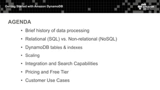
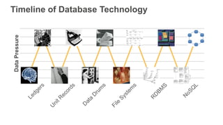
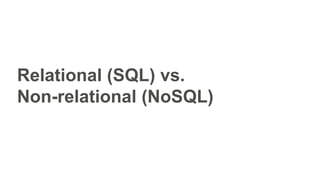
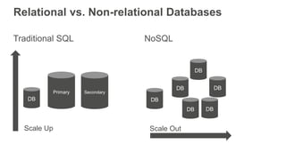
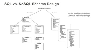
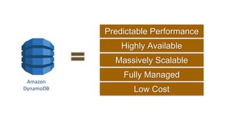
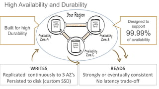
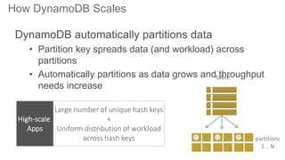
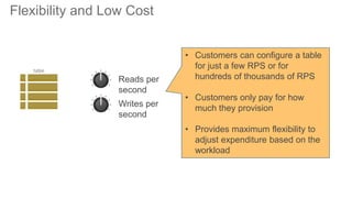
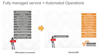
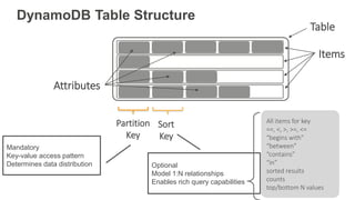
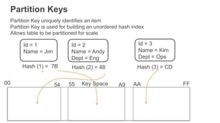
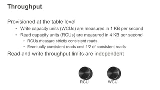
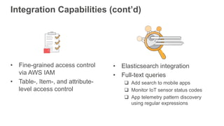
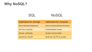
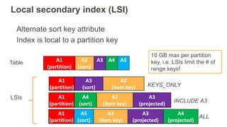
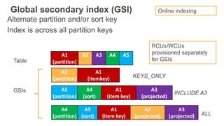
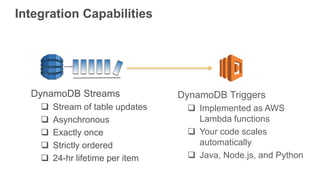
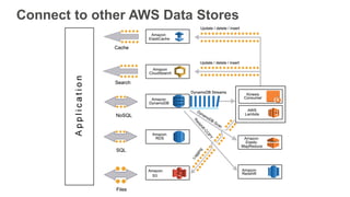
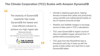
Jim Scharf will give a presentation on Getting Started with Amazon DynamoDB. The presentation will provide a brief history of data processing, compare relational and non-relational databases, explain DynamoDB tables and indexes, scaling, integration capabilities, pricing, and include customer use cases. The agenda also includes time for Q&A.

1. Jim Scharf
General Manager, DynamoDB
Time : 10:10 – 10:50
Getting Started with Amazon
DynamoDB

2. Getting Started with Amazon DynamoDB
AGENDA
• Brief history of data processing
• Relational (SQL) vs. Non-relational (NoSQL)
• DynamoDB tables & indexes
• Scaling
• Integration and Search Capabilities
• Pricing and Free Tier
• Customer Use Cases

3. Timeline of Database Technology

4. Data Volume Since 2010
• 90% of stored data generated in
last 2 years
• 1 Terabyte of data in 2010 equals
6.5 Petabytes today
• Linear correlation between data
pressure and technical innovation
• No reason these trends will not
continue over time

5. Technology Adoption and the Hype Curve

6. Relational (SQL) vs.
Non-relational (NoSQL)

7. Amazon’s Path to DynamoDB
RDBMS
DynamoDB

8. Relational vs. Non-relational Databases
Traditional SQL NoSQL
DB
Primary Secondary
Scale Up
DB
DB
DBDB
DB DB
Scale Out

9. Why NoSQL?
Optimized for storage Optimized for compute
Normalized/relational Denormalized/hierarchical
Ad hoc queries Instantiated views
Scale vertically Scale horizontally
Good for OLAP Built for OLTP at scale
SQL NoSQL

10. SQL vs. NoSQL Schema Design
NoSQL design optimizes for
Compute instead of storage

11. NoSQL Opportunity

12. SQL NoSQL
Evolution of Databases

13. Amazon
DynamoDB
Fully Managed
Low Cost
Predictable Performance
Massively Scalable
Highly Available

14. Consistently Low Latency At Scale
PREDICTABLE
PERFORMANCE!!!

15. High Availability and Durability
WRITES
Replicated continuously to 3 AZ’s
Persisted to disk (custom SSD)
READS
Strongly or eventually consistent
No latency trade-off
Designed to
support
99.99%
of availability
Built for high
Durability

16. How DynamoDB Scales
partitions
1 .. N
table
DynamoDB automatically partitions data
• Partition key spreads data (and workload) across
partitions
• Automatically partitions as data grows and throughput
needs increase
Large number of unique hash keys
+
Uniform distribution of workload
across hash keys
High-scale
Apps

17. Flexibility and Low Cost
Reads per
second
Writes per
second
table
• Customers can configure a table
for just a few RPS or for
hundreds of thousands of RPS
• Customers only pay for how
much they provision
• Provides maximum flexibility to
adjust expenditure based on the
workload

18. Fully managed service = Automated Operations
DB hosted on premise DB hosted on Amazon EC2

19. Fully managed service = Automated Operations
DB hosted on premise DynamoDB

20. DynamoDB Tables & Indexes

21. DynamoDB Table Structure
Table
Items
Attributes
Partition
Key
Sort
Key
Mandatory
Key-value access pattern
Determines data distribution Optional
Model 1:N relationships
Enables rich query capabilities
All items for key
==, <, >, >=, <=
“begins with”
“between”
“contains”
“in”
sorted results
counts
top/bottom N values

22. 00 55 A954 FFAA
Partition Keys
Partition Key uniquely identifies an item
Partition Key is used for building an unordered hash index
Allows table to be partitioned for scale
Id = 1
Name = Jim
Hash (1) = 7B
Id = 2
Name = Andy
Dept = Eng
Hash (2) = 48
Id = 3
Name = Kim
Dept = Ops
Hash (3) = CD
Key Space

23. Partition:Sort Key
Partition:Sort Key uses two attributes together to uniquely identify an Item
Within unordered hash index, data is arranged by the sort key
No limit on the number of items (∞) per partition key
• Except if you have local secondary indexes
00:0 FF:∞
Hash (2) = 48
Customer# = 2
Order# = 10
Item = Pen
Customer# = 2
Order# = 11
Item = Shoes
Customer# = 1
Order# = 10
Item = Toy
Customer# = 1
Order# = 11
Item = Boots
Hash (1) = 7B
Customer# = 3
Order# = 10
Item = Book
Customer# = 3
Order# = 11
Item = Paper
Hash (3) = CD
55 A9:∞54:∞ AA
Partition 1 Partition 2 Partition 3

24. Partitions are three-way replicated
Id = 2
Name = Andy
Dept = Engg
Id = 3
Name = Kim
Dept = Ops
Id = 1
Name = Jim
Id = 2
Name = Andy
Dept = Engg
Id = 3
Name = Kim
Dept = Ops
Id = 1
Name = Jim
Id = 2
Name = Andy
Dept = Engg
Id = 3
Name = Kim
Dept = Ops
Id = 1
Name = Jim
Replica 1
Replica 2
Replica 3
Partition 1 Partition 2 Partition N

25. Local secondary index (LSI)
Alternate sort key attribute
Index is local to a partition key
A1
(partition)
A3
(sort)
A2
(item key)
A1
(partition)
A2
(sort)
A3 A4 A5
LSIs A1
(partition)
A4
(sort)
A2
(item key)
A3
(projected)
Table
KEYS_ONLY
INCLUDE A3
A1
(partition)
A5
(sort)
A2
(item key)
A3
(projected)
A4
(projected)
ALL
10 GB max per partition
key, i.e. LSIs limit the # of
range keys!

26. Global secondary index (GSI)
Alternate partition and/or sort key
Index is across all partition keys
A1
(partition)
A2 A3 A4 A5
GSIs A5
(partition)
A4
(sort)
A1
(item key)
A3
(projected)
Table
INCLUDE A3
A4
(partition)
A5
(sort)
A1
(item key)
A2
(projected)
A3
(projected) ALL
A2
(partition)
A1
(itemkey) KEYS_ONLY
RCUs/WCUs
provisioned separately
for GSIs
Online indexing

27. How do GSI updates work?
Table
Primary
table
Primary
table
Primary
table
Primary
table
Global
Secondary
Index
Client
2. Asynchronous
update (in progress)
If GSIs don’t have enough write capacity, table writes will be throttled!

28. LSI or GSI?
LSI can be modeled as a GSI
If data size in an item collection > 10 GB, use GSI
If eventual consistency is okay for your scenario, use
GSI!

29. Scaling

30. Scaling
Throughput
• Provision any amount of throughput to a table
Size
• Add any number of items to a table
• Max item size is 400 KB
• LSIs limit the number of range keys due to 10 GB limit
Scaling is achieved through partitioning

31. Throughput
Provisioned at the table level
• Write capacity units (WCUs) are measured in 1 KB per second
• Read capacity units (RCUs) are measured in 4 KB per second
• RCUs measure strictly consistent reads
• Eventually consistent reads cost 1/2 of consistent reads
Read and write throughput limits are independent
WCURCU

32. Partitioning math
In the future, these details might change…
Number of Partitions
By Capacity (Total RCU / 3000) + (Total WCU / 1000)
By Size Total Size / 10 GB
Total Partitions CEILING(MAX (Capacity, Size))

33. Partitioning example Table size = 8 GB, RCUs = 5000, WCUs = 500
RCUs per partition = 5000/3 = 1666.67
WCUs per partition = 500/3 = 166.67
Data/partition = 10/3 = 3.33 GB
RCUs and WCUs are uniformly
spread across partitions
Number of Partitions
By Capacity (5000 / 3000) + (500 / 1000) = 2.17
By Size 8 / 10 = 0.8
Total Partitions CEILING(MAX (2.17, 0.8)) = 3

34. To learn more, please attend:
Deep Dive on DynamoDB
Room E450a, 11:45am-12:45pm
Rick Houlihan, Principal Solutions Architect

35. Integration Capabilities
DynamoDB Triggers
 Implemented as AWS
Lambda functions
 Your code scales
automatically
 Java, Node.js, and Python
DynamoDB Streams
 Stream of table updates
 Asynchronous
 Exactly once
 Strictly ordered
 24-hr lifetime per item

36. Integration Capabilities (cont’d)
• Elasticsearch integration
• Full-text queries
 Add search to mobile apps
 Monitor IoT sensor status codes
 App telemetry pattern discovery
using regular expressions
• Fine-grained access control
via AWS IAM
• Table-, Item-, and attribute-
level access control

37. Connect to other AWS Data Stores

38. Customer Use Cases

39. Over 200 million usersOver 4 billion items stored
Millions of ads per month
Cross-device ad solutions
130+ million new users in 1 year
150+ million messages per month
Process requests in milliseconds High-performance ads
Statcast uses burst scalability
for many games on a single day
Flexibility for fast growth
Web clickstream insights
Specialty online & retail stores
Over 5 billion items
processed daily
About 200 million messages
processed daily
Cognitive training
Job-matching platform
5+ million registered users
Mobile game analytics
10M global users
Home security
Wearable and IoT
solutions
170,000 concurrent players

40. The Climate Corporation (TCC) Scales with Amazon DynamoDB
The Climate Corporation is a San Francisco-based
company that examines weather data to help farmers
optimize their decision-making.
The elasticity of DynamoDB
read/write Ops made
DynamoDB the fastest and
most efficient solution to
achieve our high ingest rate
Mohamed Ahmed
Director of Engineering,
Site Reliability Engineering & Data Analytics
The Climate Corporation
”
“ • Climate is digitizing agriculture, helping
farmers increase their yields and productivity
using scientific and mathematical models on
top of massive amounts of data
• Weather and Satellite imagery is one large
source of data used in TCC’s calculations
• TCC uses DynamoDB to ingest a burst of
data and satellite images retrieved from 3rd
parties before processing them
• TCC goes from few Read/Write Ops to
thousands each day to keep up with the
bursts of data written and read from it main
DynamoDB tables

41. Thank you!

42. Agenda
• Brief history of data processing
• Relational (SQL) vs. Non-relational (NoSQL)
• DynamoDB tables & indexes
• Scaling
• Int and Search Capabilities
• Pricing and Free Tier
• Customer Use Cases

43. Timeline of Database Technology

44. Data Volume Since 2010
• 90% of stored data generated in
last 2 years
• 1 Terabyte of data in 2010 equals
6.5 Petabytes today
• Linear correlation between data
pressure and technical innovation
• No reason these trends will not
continue over time

45. Technology Adoption and the Hype Curve

46. Relational (SQL) vs.
Non-relational (NoSQL)

47. Amazon’s Path to DynamoDB
RDBMS
DynamoDB

48. Relational vs. Non-relational Databases
Traditional SQL NoSQL
DB
Primary Secondary
Scale Up
DB
DB
DBDB
DB DB
Scale Out

49. Why NoSQL?
Optimized for storage Optimized for compute
Normalized/relational Denormalized/hierarchical
Ad hoc queries Instantiated views
Scale vertically Scale horizontally
Good for OLAP Built for OLTP at scale
SQL NoSQL

50. SQL vs. NoSQL Schema Design
NoSQL design optimizes for
Compute instead of storage

51. NoSQL Opportunity

52. SQL NoSQL
Evolution of Databases

53. The Year of the Monkey
DynamoDB!

54. Amazon
DynamoDB
Fully Managed
Low Cost
Predictable Performance
Massively Scalable
Highly Available

55. Consistently Low Latency At Scale
PREDICTABLE
PERFORMANCE!!!

56. High Availability and Durability
WRITES
Replicated continuously to 3 AZ’s
Persisted to disk (custom SSD)
READS
Strongly or eventually consistent
No latency trade-off
Designed to
support
99.99%
of availability
Built for high
Durability

57. How DynamoDB Scales
partitions
1 .. N
table
DynamoDB automatically partitions data
• Partition key spreads data (and workload) across
partitions
• Automatically partitions as data grows and throughput
needs increase
Large number of unique hash keys
+
Uniform distribution of workload
across hash keys
High-scale
Apps

58. Flexibility and Low Cost
Reads per
second
Writes per
second
table
• Customers can configure a table
for just a few RPS or for
hundreds of thousands of RPS
• Customers only pay for how
much they provision
• Provides maximum flexibility to
adjust expenditure based on the
workload

59. Fully managed service = Automated Operations
DB hosted on premise DB hosted on Amazon EC2

60. Fully managed service = Automated Operations
DB hosted on premise DynamoDB

61. DynamoDB Tables & Indexes

62. DynamoDB Table Structure
Table
Items
Attributes
Partition
Key
Sort
Key
Mandatory
Key-value access pattern
Determines data distribution Optional
Model 1:N relationships
Enables rich query capabilities
All items for key
==, <, >, >=, <=
“begins with”
“between”
“contains”
“in”
sorted results
counts
top/bottom N values

63. 00 55 A954 FFAA
Partition Keys
Partition Key uniquely identifies an item
Partition Key is used for building an unordered hash index
Allows table to be partitioned for scale
Id = 1
Name = Jim
Hash (1) = 7B
Id = 2
Name = Andy
Dept = Eng
Hash (2) = 48
Id = 3
Name = Kim
Dept = Ops
Hash (3) = CD
Key Space

64. Partition:Sort Key
Partition:Sort Key uses two attributes together to uniquely identify an Item
Within unordered hash index, data is arranged by the sort key
No limit on the number of items (∞) per partition key
• Except if you have local secondary indexes
00:0 FF:∞
Hash (2) = 48
Customer# = 2
Order# = 10
Item = Pen
Customer# = 2
Order# = 11
Item = Shoes
Customer# = 1
Order# = 10
Item = Toy
Customer# = 1
Order# = 11
Item = Boots
Hash (1) = 7B
Customer# = 3
Order# = 10
Item = Book
Customer# = 3
Order# = 11
Item = Paper
Hash (3) = CD
55 A9:∞54:∞ AA
Partition 1 Partition 2 Partition 3

65. Partitions are three-way replicated
Id = 2
Name = Andy
Dept = Engg
Id = 3
Name = Kim
Dept = Ops
Id = 1
Name = Jim
Id = 2
Name = Andy
Dept = Engg
Id = 3
Name = Kim
Dept = Ops
Id = 1
Name = Jim
Id = 2
Name = Andy
Dept = Engg
Id = 3
Name = Kim
Dept = Ops
Id = 1
Name = Jim
Replica 1
Replica 2
Replica 3
Partition 1 Partition 2 Partition N

66. Local secondary index (LSI)
Alternate sort key attribute
Index is local to a partition key
A1
(partition)
A3
(sort)
A2
(item key)
A1
(partition)
A2
(sort)
A3 A4 A5
LSIs A1
(partition)
A4
(sort)
A2
(item key)
A3
(projected)
Table
KEYS_ONLY
INCLUDE A3
A1
(partition)
A5
(sort)
A2
(item key)
A3
(projected)
A4
(projected)
ALL
10 GB max per partition
key, i.e. LSIs limit the # of
range keys!

67. Global secondary index (GSI)
Alternate partition and/or sort key
Index is across all partition keys
A1
(partition)
A2 A3 A4 A5
GSIs A5
(partition)
A4
(sort)
A1
(item key)
A3
(projected)
Table
INCLUDE A3
A4
(partition)
A5
(sort)
A1
(item key)
A2
(projected)
A3
(projected) ALL
A2
(partition)
A1
(itemkey) KEYS_ONLY
RCUs/WCUs
provisioned separately
for GSIs
Online indexing

68. How do GSI updates work?
Table
Primary
table
Primary
table
Primary
table
Primary
table
Global
Secondary
Index
Client
2. Asynchronous
update (in progress)
If GSIs don’t have enough write capacity, table writes will be throttled!

69. LSI or GSI?
LSI can be modeled as a GSI
If data size in an item collection > 10 GB, use GSI
If eventual consistency is okay for your scenario, use
GSI!

70. Scaling

71. Scaling
Throughput
• Provision any amount of throughput to a table
Size
• Add any number of items to a table
• Max item size is 400 KB
• LSIs limit the number of range keys due to 10 GB limit
Scaling is achieved through partitioning

72. Throughput
Provisioned at the table level
• Write capacity units (WCUs) are measured in 1 KB per second
• Read capacity units (RCUs) are measured in 4 KB per second
• RCUs measure strictly consistent reads
• Eventually consistent reads cost 1/2 of consistent reads
Read and write throughput limits are independent
WCURCU

73. Partitioning math
In the future, these details might change…
Number of Partitions
By Capacity (Total RCU / 3000) + (Total WCU / 1000)
By Size Total Size / 10 GB
Total Partitions CEILING(MAX (Capacity, Size))

74. Partitioning example Table size = 8 GB, RCUs = 5000, WCUs = 500
RCUs per partition = 5000/3 = 1666.67
WCUs per partition = 500/3 = 166.67
Data/partition = 10/3 = 3.33 GB
RCUs and WCUs are uniformly
spread across partitions
Number of Partitions
By Capacity (5000 / 3000) + (500 / 1000) = 2.17
By Size 8 / 10 = 0.8
Total Partitions CEILING(MAX (2.17, 0.8)) = 3

75. To learn more, please attend:
Deep Dive on DynamoDB
Room E450a, 11:45am-12:45pm
Rick Houlihan, Principal Solutions Architect

76. Integration Capabilities
DynamoDB Triggers
 Implemented as AWS
Lambda functions
 Your code scales
automatically
 Java, Node.js, and Python
DynamoDB Streams
 Stream of table updates
 Asynchronous
 Exactly once
 Strictly ordered
 24-hr lifetime per item

77. Integration Capabilities (cont’d)
• Elasticsearch integration
• Full-text queries
 Add search to mobile apps
 Monitor IoT sensor status codes
 App telemetry pattern discovery
using regular expressions
• Fine-grained access control
via AWS IAM
• Table-, Item-, and attribute-
level access control

78. Connect to other AWS Data Stores

79. Customer Use Cases

80. Over 200 million usersOver 4 billion items stored
Millions of ads per month
Cross-device ad solutions
130+ million new users in 1 year
150+ million messages per month
Process requests in milliseconds High-performance ads
Statcast uses burst scalability
for many games on a single day
Flexibility for fast growth
Web clickstream insights
Specialty online & retail stores
Over 5 billion items
processed daily
About 200 million messages
processed daily
Cognitive training
Job-matching platform
5+ million registered users
Mobile game analytics
10M global users
Home security
Wearable and IoT
solutions
170,000 concurrent players

81. The Climate Corporation (TCC) Scales with Amazon DynamoDB
The Climate Corporation is a San Francisco-based
company that examines weather data to help farmers
optimize their decision-making.
The elasticity of DynamoDB
read/write Ops made
DynamoDB the fastest and
most efficient solution to
achieve our high ingest rate
Mohamed Ahmed
Director of Engineering,
Site Reliability Engineering & Data Analytics
The Climate Corporation
”
“ • Climate is digitizing agriculture, helping
farmers increase their yields and productivity
using scientific and mathematical models on
top of massive amounts of data
• Weather and Satellite imagery is one large
source of data used in TCC’s calculations
• TCC uses DynamoDB to ingest a burst of
data and satellite images retrieved from 3rd
parties before processing them
• TCC goes from few Read/Write Ops to
thousands each day to keep up with the
bursts of data written and read from it main
DynamoDB tables

82. Thank you!