This thesis examines building-integrated renewable energy systems installed at the EcoSmart show village developed by Barratt Developments PLC. Various renewable systems were monitored over a 12-month period to analyze their performance under realistic conditions. The systems included photovoltaics, solar thermal collectors, micro wind turbines, ground source heat pumps, and micro-combined heat and power. Measured energy generation and consumption data was used to validate performance models of the systems. Financial and carbon savings were estimated based on performance. The thesis provides recommendations for improving system designs to maximize benefits based on lessons learned.


![20
FIGURE 11.18: LONGITUDINAL TURBULENCE (HOURLY STANDARD DEVIATION OF WIND SPEED) DURING
GENERATING TIMES OF BOTH TURBINES OVER A 4-WEEK SAMPLE PERIOD IN 2007....................257
FIGURE 11.19: LATERAL TURBULENCE FOR COMBINED PERIODS OF ENERGY GENERATION ONLY, OVER A 4-
WEEK SAMPLE PERIOD IN 2007 ................................................................................258
FIGURE 11.20: LATERAL TURBULENCE FOR COMBINED PERIODS OF ZERO GENERATION ONLY, OVER A 4-WEEK
SAMPLE PERIOD IN 2007 .......................................................................................258
FIGURE 11.21: STATISTICS FROM FEEDBACK QUESTIONNAIRE (SOURCE: SMS MARKET RESEARCH SUMMARY
REPORT) ...........................................................................................................262
FIGURE 12.1: VERTICAL U SYSTEM (LEFT) AND HORIZONTAL SLINKY-TYPE SYSTEM (RIGHT) (SOURCE:
CURTIS
285, 2001) ...............................................................................................266
FIGURE 12.2: COMPRESSION / EXPANSION CIRCUIT OF GSHP SYSTEM (SOURCE: CALOREX GSHP USER
MANUAL) ...........................................................................................................267
FIGURE 12.3: GSHP UNIT (LEFT) AND BOREHOLE/PILING OPERATIONS (RIGHT) ................................268
FIGURE 12.4: MODELLED SOIL TEMPERATURE VARIATION IN UK (SOURCE: DOHERTY ET AL
291, 2004)......272
FIGURE 12.5: SOIL TEMPERATURE VARIATIONS IN BRITAIN (SOURCE: BS EN15450290) .....................272
FIGURE 12.6: TEMPERATURE PROFILE IN °C NEAR BOREHOLE (BHE) AT BEGINNING [LEFT] AND AFTER 3
MONTHS OPERATION DURING WINTER IN GERMANY [RIGHT] (SOURCE: RAYBACH & SANNER
283, 2000)
......................................................................................................................273
FIGURE 12.7: PALMERSTON INTERNAL TEMPERATURE VARIATIONS DURING WINTER PERIOD ....................280
FIGURE 12.8: PALMERSTON INTERNAL HUMIDITY VARIATIONS DURING WINTER PERIOD .........................280
FIGURE 12.9: MALVERN HEAT PUMP POWER CONSUMPTION AND TEMPERATURE VARIATIONS ....................281
FIGURE 12.10: TEMPERATURE DIFFERENCE BETWEEN MALVERN GSHP FLOW AND RETURN PIPES..............283
FIGURE 12.11: STATISTICS FROM FEEDBACK QUESTIONNAIRE (SOURCE: SMS MARKET RESEARCH SUMMARY
REPORT) ...........................................................................................................284
FIGURE 13.1: WHISPERGEN MCHP SYSTEM AT ECOSMART SHOW VILLAGE ......................................289
FIGURE 13.2: WHISPERGEN MCHP SYSTEM (SOURCE: WHISPERGEN TECHNICAL SPECIFICATION BROCHURE)
......................................................................................................................290
FIGURE 13.3: COMPARISON OF BUCKINGHAM DATA .................................................................295
FIGURE 13.4: BUCKINGHAM HEAT AND ELECTRICITY OUTPUT COMPARED TO GAS CONSUMPTION ...............296
FIGURE 13.5: INTERNAL TEMPERATURE OF MCHP-CONTROLLED HOMES, APRIL-JULY 2007 ...................296
FIGURE 13.6: INTERNAL TEMPERATURE OF MCHP-CONTROLLED HOMES, JANUARY-APRIL 2007...............297
FIGURE 13.7: ELECTRICAL EFFICIENCY AND OVERALL EFFICIENCY OF BUCKINGHAM SYSTEM ....................298
FIGURE 13.8: HEAT AND ELECTRICITY OUTPUT COMPARED TO GAS CONSUMPTION OF EDINBURGH SYSTEM ...300
FIGURE 13.9: ELECTRICAL EFFICIENCY AND OVERALL EFFICIENCY OF EDINBURGH SYSTEM ......................302
FIGURE 13.10: GAS CONSUMPTION AND ELECTRICITY GENERATION OVER ONE CYCLE ...........................303
FIGURE 13.11: STATISTICS FROM FEEDBACK QUESTIONNAIRE (SOURCE: SMS MARKET RESEARCH SUMMARY
REPORT) ...........................................................................................................304](https://image.slidesharecdn.com/2a840ac0-7978-44a8-bd44-7f61960c2437-141126174221-conversion-gate02/85/Alex-Glass-EngD-Thesis-20-320.jpg)


![203
Q = mc [( T − T ) + ( T − T )]
(10.30)
gain f top initial ,top bottom initial ,bottom 1
2
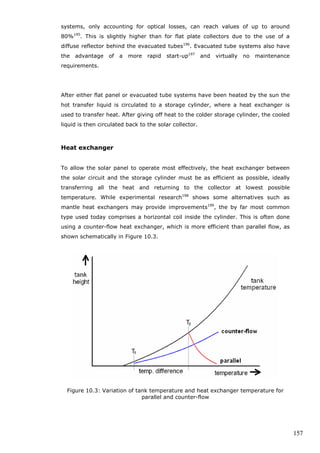
The results were summed to give daily totals and converted to kWh. The energy
gain based on cylinder temperature is given in Table 10.W labelled ‘Sensors
(cylinder temp.)’.
A comparison between the manually recorded data and the model output is
given in Table 10.W and Figure 10.22. For data gaps in the cumulative manual
data, which result from periods of absence from the house, the ‘Daily’ value
represents the cumulative value over the preceding gap. ‘Manual data’ refers to
data recorded from the control panel.
Table 10.W: Comparison between measured and modelled generation of Test
System 1
Manual data (kWh) Sensors (kWh) Model (kWh)
Cumulative Daily (cylinder temp.) Solar Solar + boiler
01/04/2010 156 2 2.4
02/04/2010 158 2 3.0 1.1 5.1
03/04/2010
04/04/2010
05/04/2010
06/04/2010
07/04/2010 174 16 12.4 8.8 11.0
08/04/2010 179 5 4.6 3.0 3.0
09/04/2010 184 5 3.6 2.8 3.2
10/04/2010 189 5 4.1 3.1 4.4
11/04/2010 193 4 4.1 4.4 4.4
12/04/2010 199 6 4.5 3.7 4.5
13/04/2010
14/04/2010 205 6 6.0 4.2 6.3
15/04/2010
16/04/2010 0.0
17/04/2010 223 18 14.3 10.2 11.3
18/04/2010 224 1 1.9 2.0 2.0
19/04/2010
20/04/2010 229 5 4.5 3.7 4.1
21/04/2010 234 5 5.3 4.0 4.0
22/04/2010
23/04/2010
24/04/2010
25/04/2010
26/04/2010 253 19 16.9 13.5 13.5
27/04/2010 258 5 3.8 3.7 3.7
28/04/2010 260 2 2.4 2.8 2.8
29/04/2010 261 1 1.2 0.6 0.6
30/04/2010 2.3 2.3
Total* 107.0 92.6 74.0 83.9
*Total does not include 30th April as no comparative data is available](https://image.slidesharecdn.com/2a840ac0-7978-44a8-bd44-7f61960c2437-141126174221-conversion-gate02/85/Alex-Glass-EngD-Thesis-204-320.jpg)


![237
The power law is able to give very similar results to the logarithmic law, hence
can be seen as an adequate alternative to calculate wind shear for a given
height within the turbulent boundary layer.
As shown by the logarithmic law and the related power law, the wind shear is
highly dependent on roughness length (z0) and surface drag coefficient (k ).
Both values in turn are highly dependent on the type of terrain. Table 11.F
gives a set of typical reference values which were adapted from the Australian
Standard for Wind Loads261, one of several reliable international standards262.
Table 11.F: Roughness length and drag coefficient for different terrain types
(Source: Australian Standard AS1170.2)
Terrain Type Roughness length z0 (m) Drag coefficient k
Very flat (snow, desert) 0.001-0.005 0.002-0.003
Open (grassland, few trees) 0.01-0.05 0.003-0.006
Suburban (buildings, height 3-5m) 0.1-0.5 0.0075-0.02
Dense urban (buildings, 10-30m) 1-5 0.03-0.3
Turbulence
The level of turbulence essentially describes the gustiness of air, and can be
measured using the standard deviation of a set of wind speeds. Equation (5.2)
for standard deviation can be re-written in terms of wind speed (u(t)), given by
equation (11.7).
1
[ ] 2
2
s ( )
(11.7)
1](https://image.slidesharecdn.com/2a840ac0-7978-44a8-bd44-7f61960c2437-141126174221-conversion-gate02/85/Alex-Glass-EngD-Thesis-238-320.jpg)


![273
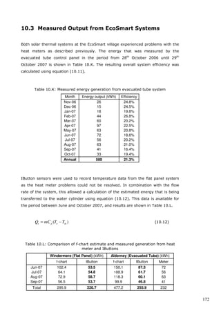
After assessing the temperature variation with depth of typical soil, it must also be
considered that the use of a GSHP means heat is extracted from the soil, and the
distribution can change over time. This has been investigated previously, and
measurements have given the change in temperature profile due to use of a
vertical GSHP system. Figure 12.6 shows soil heat distribution after 3 months of
GSHP operation during the winter in Germany283.
Figure 12.6: Temperature profile in °C near borehole (BHE) at beginning [left] and
after 3 months operation during Winter in Germany [right] (Source: Raybach
Sanner283, 2000)
Figure 12.6 shows that the temperature decreases significantly in immediate
proximity to the borehole, particularly within a 5m range around it. Other
research295 confirms this, where modelling of the ground temperature using a
reverse-cycle heat pump in Hong-Kong resulted in significant temperature
variations predominantly within a 5m range around the borehole. After conducting
a detailed investigation, Hopkirk Kaelin298 suggested that if several vertical heat-exchangers
are placed in close proximity they should at least be 5m apart, ideally
15m, to avoid any thermal interference.](https://image.slidesharecdn.com/2a840ac0-7978-44a8-bd44-7f61960c2437-141126174221-conversion-gate02/85/Alex-Glass-EngD-Thesis-275-320.jpg)