This document is a thesis submitted by Aaron Outhwaite to Dalhousie University in partial fulfillment of the requirements for a Master of Applied Sciences degree. The thesis characterizes the design and modeling of a building-integrated microalgae photobioreactor (BIMP) system. It discusses BIMP design fundamentals, including growth limiting factors like light, temperature, nutrients, and carbon. It also covers BIMP modeling fundamentals, growth rate expressions, and dynamics of light, temperature, nutrients, and carbon dioxide in the system. Several chapters then present mathematical models of light and temperature dynamics in a BIMP and results of the models.

1. THE CHARACTERIZATION OF A BUILDING-INTEGRATED MICROALGAE
PHOTOBIOREACTOR
by
Aaron Outhwaite
Submitted in partial fulfilment of the requirements
for the degree of Master of Applied Sciences
at
Dalhousie University
Halifax, Nova Scotia
August 2015
© Copyright by Aaron Outhwaite, 2015

2. ii
Table of Contents
List of Tables............................................................................................................................................. v
List of Figures..........................................................................................................................................vi
Abstract ...................................................................................................................................................... x
List of Abbreviations Used .................................................................................................................xi
Acknowledgements..............................................................................................................................xii
Chapter 1 Introduction...................................................................................................................1
1.1 Characterization of a Building-Integrated Microalgae Photobioreactor ..............5
Chapter 2 BIMP Design Fundamentals ....................................................................................7
2.1 Introduction..................................................................................................................................7
2.2 BIMP Design Characterization...............................................................................................8
2.3 Growth Limiting Factors....................................................................................................... 16
2.3.1 Light...................................................................................................................................... 16
2.3.2 Temperature ..................................................................................................................... 19
2.3.3 Nutrients............................................................................................................................. 21
2.3.4 Carbon ................................................................................................................................. 24
2.4 Discussion................................................................................................................................... 26
Chapter 3 BIMP Modeling Fundamentals ............................................................................. 28
3.1 Introduction............................................................................................................................... 28
3.2 System Description................................................................................................................. 29
3.3 BIMP System Growth Modeling ......................................................................................... 30
3.3.1 Continuous Photobioreactor....................................................................................... 31
3.3.2 Fed-batch Photobioreactor.......................................................................................... 34
3.4 Growth Rate Expressions ..................................................................................................... 35
3.4.1 Monod Growth Rate ....................................................................................................... 35
3.4.2 Haldane Growth Rate..................................................................................................... 37
3.4.3 Maximum Growth Rate................................................................................................. 39
3.4.4 Multiplicative Growth Rate ......................................................................................... 40
3.5 BIMP Light Dynamics............................................................................................................. 43
3.5.2 Light-Dependent Growth Rate ................................................................................... 49

3. iii
3.6 BIMP Temperature Dynamics............................................................................................. 51
3.6.1 Temperature-Dependent Growth Rate................................................................... 56
3.7 BIMP Nutrient Dynamics...................................................................................................... 56
3.7.1 Rainwater........................................................................................................................... 58
3.7.2 Human Urine..................................................................................................................... 60
3.7.3 Nutrient-Dependent Growth rate ............................................................................. 61
3.8 BIMP CO2 Dynamics................................................................................................................ 62
3.8.1 Biological Phase............................................................................................................... 63
3.8.2 Gas Phase............................................................................................................................ 63
3.8.3 Liquid Phase...................................................................................................................... 66
3.8.4 CO2-Dependent Growth Rate...................................................................................... 68
3.9 Discussion................................................................................................................................... 68
Chapter 4 Modeling Light Dynamics in a BIMP System.................................................. 70
4.1 Introduction............................................................................................................................... 70
4.2 System Description................................................................................................................. 70
4.3 Mathematical Model............................................................................................................... 71
4.3.1 Solar model........................................................................................................................ 72
4.3.2 Biological model .............................................................................................................. 72
4.4 Results.......................................................................................................................................... 73
4.5 Sensitivity Analysis................................................................................................................. 76
4.6 Discussion................................................................................................................................... 76
Chapter 5 Modeling Temperature Dynamics in a BIMP System .................................. 79
5.1 Introduction............................................................................................................................... 79
5.2 System Description................................................................................................................. 79
5.3 Mathematical Model............................................................................................................... 81
5.3.1 Temperature model........................................................................................................ 81
5.3.2 Biological model .............................................................................................................. 83
5.4 Results.......................................................................................................................................... 83
5.5 Sensitivity Analysis................................................................................................................. 86
5.6 Discussion................................................................................................................................... 86

4. iv
Chapter 6 Conclusions................................................................................................................. 88
References.............................................................................................................................................. 93
Appendix A Equilibrium Equations for BIMP Nutrient System.................................104
Appendix B MATLAB Code.......................................................................................................107
B.1 Monod........................................................................................................................................107
B.2 Haldane .....................................................................................................................................109
B.3 Light Main.................................................................................................................................110
B.4 Solar Function.........................................................................................................................112
B.5 Light-Temperature Main....................................................................................................114
B.6 Temperature function .........................................................................................................116

5. v
List of Tables
Table 2.1: Design Features for Outdoor Microalgae PBR Systems
(adapted Ugwu et al., 2008). 9
Table 2.2: Classification of Different Wastewater Effluent in Terms of
Total Kjeldahl Nitrogen (TKN) and Total Phosphorus (TP) (adapted
from Cai et al., 2013; Christenson and Sims, 2011). 23
Table 3.1: Reported Maximum Specific Growth Rate 𝜇 𝑚𝑎𝑥 (h-1) Values
for PBR Systems Growing the Microalgae Species C. vulgaris. 40
Table 3.2: Composition of Fresh Human Urine (FMU) and Stored
Human Urine (SHU) (adapted from Udert et al., 2003a). 60
Table 4.1: Meteorological Data for Halifax Nova Scotia Canada
(adapted from Green Power Labs, 2009; Duffie and Beckman, 2006). 72
Table 4.2: Summary of BIMP Light Model Parameters for Microalgae
Species C. vulgaris. 73
Table 4.3: Final BIMP Biomass Concentrations After seven-day
Growth Simulation for the Four Equinox Months When Starting from
a Concentration of 1 g L-1 Microalgae Biomass in the System. 75
Table 5.1: Outdoor Temperature Statistics and Double Cosine Model
Calibration Data for Halifax Nova Scotia Canada (Environment
Canada, 2015; Chow and Levermore, 2007). 81
Table 5.2: Summary of BIMP Heat Transfer Model Parameters. 82
Table 5.3: Summary of BIMP Temperature Model Parameters for
Microalgae Species C. vulgaris. 83
Table 5.4: Final BIMP Biomass Concentrations after Seven-Day
Growth Simulation for the Four Equinox Months When Starting from
a Concentration of 1 g L-1 Microalgae Biomass in the System. 85
Table A.1: Equilibrium Reactions for BIMP Nutrient System 106

6. vi
List of Figures
Fig. 1.1. The ecological footprint of the 29 largest cities in the Baltic
region of Europe, showing ecosystem appropriation for city resource
production (left), and ecosystem appropriation for city waste
assimilation (adapted from Folke et al., 1997). 2
Fig. 1.2. Ecological Life Support System Concept. 4
Fig. 2.1. Examples of outdoor microalgae PBR systems, including (A)
open pond (B) flat- plate (C) horizontal tubular (D) vertical column. 8
Fig. 2.2. BBS process flow diagrams for BIMP integration within the
built environment. External environmental factors include (1) Sunlight
(2) Outdoor temperature, and (3) Precipitation. Habitation dynamics
include (4) Source separated urine (5) Low quality indoor air, and (6)
Indoor Temperature. BBS dynamics include the generation and
discharge of (7) Vermicompost (8) Municipal solid waste, and (9)
Greywater, and requires the input of (10) External foodstuffs. BBS
influent streams to the BIMP include (11) Nutrients (12) CO2, and (13)
Electricity, while BIMP output to the BBS for recovery include (14) High
quality indoor air, (15) Heat, and (16) Microalgae effluent. 11
Fig. 2.3. Schematic diagram of BIMP system within a theoretical BBS
construct. 12
Fig. 2.4. Schematic diagram of metabolism requirements within a
theoretical BBS construct. 13
Fig. 2.5. Schematic diagram of food production system within
theoretical BBS construct. 14
Fig. 2.6. Schematic diagram of water usage within theoretical BBS
construct. 15
Fig. 2.7. Schematic diagram of energy recovery within theoretical BBS
construct. 16
Fig. 2.8. Microalgae growth rate as a function of light intensity and
culture depth in flat-plate PBR. 𝐼𝑐 light compensation point; 𝐼𝑠 light
saturation intensity; 𝐼ℎ light intensity value for photoinhibition onset;
𝜇 𝑚𝑎𝑥 maximum microalgal growth rate; 𝜇 𝑑 microalgae loss rate
(adapted from Grobbelaar, 2010; Ogbonna and Tanaka, 2000). 18

7. vii
Fig. 2.9. Variation of optimal light intensity 𝐼 𝑜𝑝𝑡 with culture
temperature 𝑇 𝑤 for freshwater microalgae species C. vulgaris
(adapted from Dauta et al., 1990). 20
Fig. 2.10. Variation of maximum microalgal growth rate 𝜇 𝑚𝑎𝑥 with
culture temperature 𝑇 𝑤 for freshwater microalgae species C. vulgaris
(adapted from Dauta et al., 1990). 21
Fig. 2.11. Biomass concentration (closed symbols) and urea
consumption of C. vulgaris for different initial urea concentrations
(open symbols) (5,:) 0.100 g L-1; (C,.) 0.200 g L-1 (adapted from
Hsieh and Wu, 2009). 23
Fig. 2.12. Comparison of the aqueous CO2 fixation ability of 25
microalgal species during batch growth (adapted from Ho et al.,
2011). 26
Fig. 3.1. Fundamental BIMP design schematic showing light and
temperature factors. 30
Fig. 3.2. Schematic diagram for continuous PBR (c-PBR) operation
during time 𝑡. 31
Fig. 3.3. Growth dynamics of algae biomass 𝑋 𝑎 (solid line) in a b-PBR
based on the availability of a growth limiting substrate 𝑆𝑖 (dash line)
over 7 days, or 𝑡 = 168 hours, for 𝑋 𝑎(𝑡 = 0) = 1 g L-1; 𝑆𝑖(𝑡 = 0) = 3
g-1; 𝜇 𝑚𝑎𝑥 = 0.05 h-1; 𝜇 𝑑 = 0.01 h-1; 𝑌𝑥/𝑠,𝑖 = 1 g 𝑋 𝑎 g-1 𝑆𝑖; and 𝐾𝑠,𝑖 = 0.5
g L-1. Variable parameterization based on an idealization of literature
values to show trend. 36
Fig. 3.4. Growth dynamics of algae biomass 𝑋 𝑎 (solid line) in a b-PBR
based on the availability of sunlight over 7 days, or 𝑡 = 168 hours, for
𝑋 𝑎(𝑡 = 0) = 1 g L-1; 𝜇 𝑚𝑎𝑥 = 0.05 h-1; 𝜇 𝑑 = 0.01 h-1; and 𝐾𝑠 = 100
µmol m-2 s-1. Sunlight described using a 12:12 daily light-dark cycle,
with 𝑆 = 200 µmol m-2 s-1 for light hours, and 𝑆 = 0 µmol m-2 s-1 for
dark hours. Variable parameterization based on an idealization of
literature values to show trend. 37
Fig. 3.5 Comparison of BIMP growth rate 𝜇 with increasing substrate
concentration 𝑆𝑖 as described using Monod kinetics (solid line) and
Haldane kinetics (dash line), for 𝜇 𝑚𝑎𝑥 = 0.05 h-1; 𝐾𝑠,𝑖 = 0.5 g L-1; and
𝐾𝑖,𝑖 = 0.5 g L-1. Variable parameterization based on an idealization of
literature values to show trend 39

8. viii
Fig. 3.6. Multiplicative growth rate dynamics of algae biomass 𝑋 𝑎
(solid line) within a b-PBR based on the availability of co-limiting
substrates 𝑆1 and 𝑆2 (dashed line) over 7 days, or 𝑡 = 168 hours. For
biomass growth 𝑋 𝑎,1 on substrate 𝑆1 (5,: respectively), 𝑋 𝑎,1(𝑡 =
0) = 1 g L-1; 𝑆1(𝑡 = 0) = 3 g-1; 𝜇 𝑚𝑎𝑥 = 0.05 h-1; 𝜇 𝑑 = 0.01 h-1; 𝑌𝑥/𝑠,1 =
1 g 𝑋 𝑎,1 g-1 𝑆1; and 𝐾𝑠,1 = 0.5 g L-1. For biomass growth 𝑋 𝑎,2 on
substrate 𝑆2 (C,. respectively), 𝑋 𝑎,2(𝑡 = 0) = 0.5 g L-1; 𝑆2(𝑡 = 0) =
1.5 g-1; 𝜇 𝑚𝑎𝑥 = 0.05 h-1; 𝜇 𝑑 = 0.01 h-1; 𝑌𝑥/𝑠,2 = 0.5 g 𝑋 𝑎,2 g-1 𝑆2; and
𝐾𝑠,2 = 0.25 g L-1. Variable parameterization based on an idealization
of literature values to show trend. 42
Fig. 4.1. Schematic for light interaction in BIMP system. 71
Fig. 4.2. A comparison between published Green Power Labs (2009)
data (dashed line) and calculated (solid line) data for the monthly
average daily full-spectrum solar radiation on a vertical surface facing
due South in Halifax Nova Scotia Canada. 74
Fig. 4.3. MATLAB simulation of BIMP biomass growth dynamics over
seven days as characterized by Monod (solid line) and Haldane
(dashed line) kinetic expressions, for spatially-averaged culture PPFD
in Halifax Nova Scotia Canada. (A) March (B) June (C) September (D)
December. Parameterization based on values given in Table 4.1 for
solar model, and Table 4.2 for biological models. 75
Fig. 4.4. Tornado plot showing the sensitivity of BIMP light-growth
model inputs when varied by ± 20% of their nominal value. Hatch bar
indicates change in parameter value of -20%. Solid bar indicates
change in parameter value of +20%. 76
Fig. 5.1 Schematic for temperature interaction in BIMP system 80
Fig. 5.2. MATLAB simulation of daily variation in outdoor
temperature (dashed line) and the resultant BIMP culture
temperature (solid line) for the four equinox months in Halifax Nova
Scotia Canada. (A) March (B) June (C) September (D) December.
Parameterization based on values given in Table 5.2. 84

9. ix
Fig. 5.3. MATLAB simulation of BIMP biomass growth dynamics over
7 days as characterized by Monod (solid line) kinetics for light, and
multiplicative (dashed line) kinetic for light-temperature, in Halifax
NS Canada. (A) March (B) June (C) September (D) December.
Parameterization based on values given in Table 4.1 for solar model,
and Tables 5.1 and 5.2 for temperature model, and Tables 4.2 and 5.3
for light and temperature biological models, respectively.
and Tables 5.1 and 5.2 for temperature model, and Tables 4.2 and 5.3
for light and temperature biological models, respectively 85

10. x
Abstract
This thesis uses an adaptive design methodology for the characterization of a building
integrated microalgae photobioreactor (BIMP) system. As an integrated building
component that mediates between the indoor and outdoor environments, the BIMP
system is novel in that no similar applications of microalgal photobioreactor (PBR)
technology are reported in the literature. As such, a preliminary analysis is needed of
the BIMP system before prototyping, to understand performance issues, and to
improve the fitness of the BIMP design itself. Here, the adaptive design methodology
utilizes a literature review to describe the key principles and growth limiting factors
in PBR systems, with a focus on light and temperature dynamics. This general analysis
is followed by the specific analysis of each of light and temperature dynamics within
the BIMP system, using mathematical modeling and simulation. These analyses are
evaluated, and used in summary to suggest methods for improving the BIMP design.

11. xi
List of Abbreviations Used
BBS Biological Building System
BIMP Building Integrated Microalgae Photobioreactor
b-PBR Batch Photobioreactor
c-PBR Continuous Photobioreactor
C Carbon
CELSS Closed Ecological Life Support System
CO2 Carbon Dioxide
CSTR Continuously-Stirred Tank Reactor
MATLAB MATrix LABoratory
MCHP Micro-Combined Heating and Power
N Nitrogen
NASA National Aeronautics and Space Administration
ODE Ordinary Differential Equation
P Phosphorus
PAR Photosynthetically Active Radiation
PBR Photobioreactor
PPFD Photosynthetically Active Photon Flux Density
TKN Total Kjeldahl Nitrogen
TP Total Phosphorus
UN United Nations

12. xii
Acknowledgements
It is with sincere appreciation that I thank my supervisory team of Dr. Stephen Kuzak
and Dr. Mark Gibson. Their expertise, perceptiveness, and patience gave foundation
to my ideas, and the opportunity to define them. I would also like to thank Dr. Susanne
Craig for her insight and provocation, and for asking the tough questions that help
solidify the theoretical underpinnings of my work.
I would like to thank my parents, whose unconditional support and generosity has
not only been invaluable to my thesis work, but also in making me the person I am
today. My extended family has also been incredibly supportive of my work, and I
thank them as well.
Finally, and most importantly, I thank my wife Elizabeth Powell. She has been, and
continues to be, my inspiration.

13. 1
Chapter 1 Introduction
A problem faced by cities globally is that buildings consume resources and generate
wastes, which impacts both the environment and health. However, re-designing
buildings so they behave as ecological machines, and bioregenerate their wastes, may
be a solution to this problem.
How buildings affect their biophysical environment is of great importance, not only
for the sustainability of the city, but also for the health and well-being of their
occupants. The study of cities as metabolic systems involves the quantification of the
inputs, outputs and storage of energy, water, nutrients, materials and wastes for an
urban region (Kennedy et al., 2010). As a primary mediator between humans and
their biophysical environments, buildings are a microcosm of urban metabolism
theory, wherein raw materials, energy and water are converted to human biomass
and wastes (Decker et al., 2000). By consuming these resources and generating waste
streams, the construction and operation of buildings account for the greatest burden
on natural resources of all the economic sectors (Kibert et al., 2000).
The impact that buildings have on their environment extends beyond the confines of
the city, impacting the biophysical makeup of a much larger area. For instance, Folke
et al. (1997) suggest that the 29 largest cities in the Baltic Sea drainage basin cover a
total area of 2,216 km2, but require open land that is approximately 200 times larger
to supply the resources they require. Even more alarming is the fact that these same
authors suggest that the amount of open land required to assimilate the nitrogen (N),
phosphorus (P), and carbon dioxide (CO2) generated as waste in these 29 cities is at
least 400 – 1000 times larger than the size of the cities themselves.

14. 2
Fig. 1.1. The ecological footprint of the 29 largest cities in the Baltic region of
Europe, showing ecosystem appropriation for city resource production (left), and
ecosystem appropriation for city waste assimilation (adapted from Folke et al.,
1997).
Contemporary urban design and infrastructure are failing to account for the drastic
increase in city population expected before 2050. According to a UN report (Heilig,
2012), between 2011 and 2050, the world population is expected to increase by 2.3
billion, moving from 6.8 billion to 9.1 billion. During this same time interval, the
population living in urban areas is projected to increase by 2.9 billion to a total of 6.3
billion, meaning that urban areas will house at least 70% of the world population by
2050. In North America – an already highly urbanized society – cities are expected to
house at least 90% of the population by 2050.
It is not anticipated that existing city drinking water resources will be able to manage
an increase in demand of such a magnitude. Further, an increase in city population

15. 3
will localize and increase atmospheric pollution such that the current health issues
associated with urban smog will only become exacerbated. The same is true for how
the vast amounts of garbage, and human liquid and solid waste generated by an urban
population is treated and disposed of. Again, it is anticipated that our already strained
waste management infrastructure will be able to cope with the additional waste
volume related to an increased global population. To put it simply, the contemporary
methods used to design and operate cities, and the buildings they contain, are not
sustainable.
Instead, a paradigm shift is required; a shift away from building typologies that are
inert, to those that are alive and form a productive part of the urban metabolism. The
building itself needs to behave as would a natural ecosystem, using the free resources
of sunlight and rainwater for the maintenance of living systems that can
bioregenerate depleted urban resources such as wastewater and CO2 without the
need to rely on – or destroy – vast exurban ecosystems. And we have a model for
these types of buildings available to us, namely the biologically-based, ecological life
support systems developed for space exploration.
The study of a BIMP system is based on life support systems developed by NASA and
the former Soviet Union for use during manned, non-orbital long-duration space
flights. These missions – expected to last at least two years – could not be effectively
supported from Earth, as any attempt to leave the atmosphere with the required
stores would be both uneconomical and technically unfeasible. As a result, a
fundamental outline of a new life support system was developed, entailing a
regenerative environment that could support human life in space using agricultural
means. The earliest successful controlled ecological life support systems (CELSS),
described schematically in Fig. 1.2 utilized a microalgae photobioreactor (PBR)
system that could (1) provide oxygen to an enclosed environment while at the same
time consume CO2 produced by occupant respiration, (2) regenerate wastewater
through the biofixation of various mineral constituents, including N and P, and (3)

16. 4
provide a continuous biomass food source for consumption (Nelson et al., 2009;
Gitelson et al., 2003; Eckart, 1996).
Fig. 1.2. Ecological Life Support System Concept.
Conceptually, a BIMP system is able to achieve the same results as the CELSS systems
here described. However, unlike the CELSS system, the design of a BIMP system must
account for both the indoor and outdoor environments. As such, the purpose of this
thesis is to characterize these environmental conditions, and to determine their effect
on the development of a BIMP prototype system.

17. 5
1.1 Characterization of a Building-Integrated Microalgae Photobioreactor
This thesis investigates the potential utilization of a building integrated microalgae
photobioreactor (BIMP) system. To convert building generated wastewater and
CO2 into useable resources, rather than discharge wastes streams into the
environment. As a preliminary step toward the development of a BIMP prototype, an
adaptive methodology is used to describe how sunlight and temperature affect the
growth of microalgae within the BIMP system. This involves the mathematical
modeling and simulation of these key factors, with a focus on improving the
robustness of the BIMP design.
Therefore, this thesis uses an adaptive design methodology for the development of a
BIMP system. An adaptive methodology attempts to remove uncertainly and improve
robustness by increasing the understanding of a design system before it is built as a
prototype. For the BIMP system, this means developing mathematical models to
describe those factors considered most likely to directly affect how a prototype might
be developed. Characterizing the BIMP system in such a manner will be achieved in
the following chapters, here summarized briefly.
In Chapter 2, the fundamental design requirements for a BIMP system are described,
including those factors that limit the growth of the microalgae within the system.
These factors are inclusive of both the ‘geographic’ and the ‘built’ and include the
access to sunlight, the culture temperature, as well as the availability of the nutrient
resources of wastewater, and CO2.
In Chapter 3, the basic methods for the characterization of the BIMP system through
mathematical modeling and dynamic simulation are presented. Included in this
chapter are the kinetic methods for describing growth limitation and inhibition, for
single or co-limited microalgae cultures in a BIMP system, based specifically on

18. 6
diurnal and seasonal dynamics for a particular geographic location, and on the built
environment within which it is placed.
Chapter 4 describes the dynamics of growth in the BIMP system based on the incident
solar radiation resource in Halifax Nova Scotia Canada. The mathematical modeling
and simulation of the biological dynamics within the BIMP system are presented.
Chapter 5 describes the dynamics of growth within the BIMP system based on both
the indoor and outdoor environments in Halifax. Modeling and simulation in this
chapter follow a methodology similar to that in Chapter 4, with the addition of the
multiplicative dynamics described in Chapter 3.
Chapter 6 summarizes the findings in Chapter 5 and 6, and several conclusions about
the design of the BIMP system are made.

19. 7
Chapter 2 BIMP Design Fundamentals
2.1 Introduction
As a novel biological building system (BBS), the BIMP system is akin to – but distinct
from – contemporary microalgae PBR technology. This chapter introduces the design
concepts used to manifest PBR systems, with a focus on how these principles affect
the development of the BIMP system.
The utilization of microalgal biomass grown in PBR systems has received
considerable attention in the literature, most notably in the production of biofuels
(Wiley et al., 2011; Mata et al., 2009; Chisti, 2007), as well as various other chemical
and food products (Borowitzka, 2013; Harun et al., 2012; Pulz and Gross, 2004). In an
effort to improve process efficiencies and reduce operating costs, microalgae PBR
systems have been studied empirically as part of a biorefinery concept. In these
studies, natural and waste resources such as sunlight and wastewater effluent are
utilized as part of the microalgal photosynthetic growth dynamic (Shurin et al., 2013;
Razzak et al., 2013; Sortana and Landis, 2011). In a similar effort, microalgae PBR
have been used within CELSS for the bioregeneration of the by-products of habitation,
including wastewater and CO2, for reuse within the enclosure (Ganzer and
Messerschmid, 2009; Gitelson et al., 2002; Eckart, 1996).
In open systems such as a biorefinery, PBR dynamics and design are dependent on
the outdoor environment, as well as on the availability of the abiotic resources such
as nutrients and CO2 needed for microalgae growth. Conversely, for closed systems
such as CELSS, PBR dynamics are dependent on the indoor environment, which
produces these same abiotic resources. For the BIMP system, an adaptive design
approach requires the careful consideration of both the indoor and outdoor
environmental factors considered most likely to affect the development of a

20. 8
prototype. The purpose of this chapter is to therefore introduce these environmental
factors using a literature review.
2.2 BIMP Design Characterization
In general, outdoor microalgae culturing systems that utilize solar energy are
designed to have a large illuminated surface area (Ugwu et al., 2008). Common
outdoor PBR of this type include open pond, horizontal tubular, vertical column, and
flat-plate systems, all of which have been reviewed extensively by other authors
(Wang et al., 2012; Carvalho et al., 2006; Tredici, 2004). An example for each of these
types of outdoor microalgae PBR systems is shown in Fig. 2.1.
Fig. 2.1. Examples of outdoor microalgae PBR systems, including (A) open pond (B)
flat- plate (C) horizontal tubular (D) vertical column.
As an integrated system in the built environment, the BIMP is designed to mediate
between the indoor and outdoor environments in the form of a façade element similar

21. 9
to a window. This makes the flat-plate type PBR the most obvious choice as the design
basis for the BIMP system. Additionally, to avoid obstructions from environmental
factors such as snow and rainwater accumulation, the BIMP system is vertically-
oriented. This will have an impact on the mathematical modeling of solar radiation,
which is described in detail in Chapter 3. The key design features for each
photobioreactor type are presented in Table 2.1.
Table 2.1: Design Features for Outdoor Microalgae PBR Systems (adapted Ugwu et
al., 2008).
Culture systems Prospects Limitations
Open ponds High illuminated surface area
Moderate cost;
Easy to clean after cultivation;
High land requirements;
Low productivity;
Low long term culture stability;
Limited control of growth conditions;
Limited to few microalgae strains;
Easily contaminated
Horizontal tubular High illuminated surface area;
Moderate productivity
High gradation for pH, O2, CO2 along tube
length;
High land requirements;
High cost
Vertical column High mass transfer;
High mixing with low shear
stress;
Moderate productivity;
Moderate scalability;
Easy to sterilize
High cost;
Low illuminated surface area;
Limited light path with increased scale
Flat-plate High illuminated surface area;
High productivity;
High mass transfer;
High mixing with low shear
stress;
Moderate cost;
Easy to sterilize
Moderate scaling issues;
Moderate temperature control issues;
Flat-plate PBR are cuboids in form, with a large transparent surface facing the
illumination source, and a short light path distance from that illumination source
through the reactor. Usually flat-plate panel PBR are placed vertically or inclined
facing the sun, though this is not always the case (Cuaresma et al., 2011). The large

22. 10
illumination surface and short light path characterize the flat-plate PBR as having a
high surface to volume ratio, which has the advantage of affording good light
distribution accessibility within the microalgae culture medium. However, in outdoor
flat-plate PBR, the solar gain afforded by the large surface area has the additional
effect of causing temperature changes in the culture medium, which must be
controlled to maintain optimal growth conditions (Richmond and Cheng-Wu, 2001).
Nutrients for microalgal metabolism are provided based on the operational mode of
the reactor; continuously for CSTR-type operation, and in sufficient density to
support sustained growth dynamics in batch- or fed-batch-type operation (Yamane,
1994). Because of the short light path and limited internal volume, agitation and
mixing in a flat-plate PBR is most often provided by mechanically sparging, thereby
creating gas-liquid dynamics similar to those found in vertical column type airlift and
bubble-column PBR (Chisti, 1989). This type of mixing has the added benefit of acting
as the delivery mechanism for aqueous CO2, a requirement for photosynthesis.
Describing the BIMP as a pseudo flat-plate PBR, and placing it within the façade means
that it has both an indoor and outdoor surface, and is therefore subject to the specific
environmental conditions at each of those locale. This is a non-trivial dilemma, for
while outdoor environmental conditions can readily be described, the indoor
environment requires a more thorough consideration. Here, a BBS concept has been
developed for the purposes of rationalizing the waste/resource dynamics as are
associated with habitation. These dynamics are described in Fig. 2.2.
The BBS concept described in Fig. 2.2 is not resolved in its entirety in this thesis, but
is instead used to orient the characterization of the BIMP system. Explicitly then, and
in summary, the geographic climate describes the amount of solar radiation incident
on the exterior BIMP vertical surface, as well as the outdoor surface temperature. The
indoor surface temperature, as well as the availability of the wastewater nutrients
and CO2 that are utilized for microalgae growth, are both characterized by the indoor
environment of the building in which the BIMP system is placed. Therefore, the four

23. 11
factors here considered to limit growth in the BIMP system are light, temperature,
nutrients and CO2, each of which is described in detail in the following section.
Fig. 2.2. BBS process flow diagrams for BIMP integration within the built
environment. External environmental factors include (1) Sunlight (2) Outdoor
temperature, and (3) Precipitation. Habitation dynamics include (4) Source separated
urine (5) Low quality indoor air, and (6) Indoor Temperature. BBS dynamics include
the generation and discharge of (7) Vermicompost (8) Municipal solid waste, and (9)
Greywater, and requires the input of (10) External foodstuffs. BBS influent streams to
the BIMP include (11) Nutrients (12) CO2, and (13) Electricity, while BIMP output to
the BBS for recovery include (14) High quality indoor air, (15) Heat, and (16)
Microalgae effluent.
Each of the five individual BBS subsystems shown in Fig. 2.2 are expanded, and
described in Fig. 2.3-2.7.

24. 12
Fig. 2.3. Schematic diagram of BIMP system within a theoretical BBS construct.

25. 13
Fig. 2.4. Schematic diagram of metabolism requirements within a theoretical BBS
construct.

26. 14
Fig. 2.5. Schematic diagram of food production system within theoretical BBS
construct.

27. 15
Fig. 2.6. Schematic diagram of water usage within theoretical BBS construct.

28. 16
Fig. 2.7. Schematic diagram of energy recovery within theoretical BBS construct.
2.3 Growth Limiting Factors
2.3.1 Light
The amount of light that can be utilized for photosynthesis is the critical factor in
determining the overall performance and bioregenerative capacity of a BIMP system.
Light is electromagnetic radiation that has a wavelength between 10 and 106 nm, of

29. 17
which the visible spectrum is between about 380–750 nm (Carvalho et al., 2011). The
radiation that is usable in photosynthesis is called photosynthetically active radiation
(PAR), and its wavelength range corresponds to the visible spectrum, or about 400–
700 nm. Of the total solar resource that is incident on the surface of the Earth, only
about 45.8% is PAR (Weyer et al., 2010). The general reaction for photosynthesis is
given in Eq. 2.1 and it describes the conversion of inorganic compounds and PAR to
organic matter and oxygen by autotrophs such as microalgae (Osborne and Geider,
1987).
𝐶𝑂2 + 𝐻2 𝑂 + 𝑝ℎ𝑜𝑡𝑜𝑛𝑠 → (𝐶𝐻2 𝑂) 𝑛 + 𝑂2 2.1
It is useful here to distinguish between the different methods of reporting light
energy. Often sunlight is described as a radiant flux energy, or irradiance, measured
in units of power per area per time such as J m-2 s-1 (Kalogirou, 2009). However, in
microalgae PBR research, irradiance is typically expressed as PAR photon flux density
(PPFD), measured in units of quanta per area per time, or µmol quanta m-2 s-1, or more
conveniently, µmol m-2 s-1 (Carvalho et al., 2011). The mathematical derivation for the
conversion of PAR radiant flux to PPFD is provided in Chapter 3, for the determination
of the maximum theoretical BIMP photosynthetic yield. However, it is noted here that
an approximate conversion factor for sunlight is 1 J m-2 s-1 PAR radiant flux equals 4.5
µmol m-2 s-1 PPFD (Masojidek et al., 2004).
In addition to the quality of light here described, the quantity of PAR incident on the
exterior BIMP vertical surface is very important in determining growth dynamics.
Consider that on a sunny day in equatorial regions the average solar radiation that
reaches the surface of the Earth is approximately 1000 J m-2 s-1 at noon (Kalogirou,
2009). Of this, approximately 450 J m-2 s-1 is PAR radiant flux, or approximately 2000
µmol m-2 s-1 PPFD. However, the growth of microalgae is optimum at PPFD of about
200 µmol m-2 s-1, or about 1/10th the daily average (Kumar et al., 2011). Any exposure
of the microalgae photosynthetic unit to light intensities above the saturation PPFD
can impair the photosynthetic complex, resulting in decreased growth rates, cell

30. 18
damage, and culture mortality (Richmond, 2004). Further, as light passes through
the depth of the microalgae culture, its intensity is attenuated, meaning that a light
source that is above saturation intensity at the culture surface may in fact become
optimal after attenuating at some culture depth 𝑑. The response of microalgae growth
to the quantity of light, or light intensity, is described in Fig. 2.8.
Fig. 2.8. Microalgae growth rate as a function of light intensity and culture depth in
flat-plate PBR. 𝐼𝑐 light compensation point; 𝐼𝑠 light saturation intensity; 𝐼ℎ light
intensity value for photoinhibition onset; 𝜇 𝑚𝑎𝑥 maximum microalgal growth rate; 𝜇 𝑑
microalgae loss rate (adapted from Grobbelaar, 2010; Ogbonna and Tanaka, 2000).
For unidirectional incident sunlight, at a culture depth 𝑑 from the illuminated surface,
the light compensation intensity 𝐼𝑐 is the light level at which the microalgal growth
rate is equally balanced by microalgal mortality, resulting in a net biomass
accumulation of zero. As the culture depth is decreased toward the illuminated
surface, more light is available for photosynthesis, and the microalgal growth rate is
accelerated. Eventually, the culture depth is sufficiently shallow such that the light
saturation intensity 𝐼𝑠 is reached, and the microalgal growth rate is at its maximum.
Any increase in the light intensity past the saturation value does not increase the

31. 19
microalgal growth rate, and in fact, at a certain inhibition light intensity 𝐼ℎ, the
microalgal growth rate can be seen to decline as a result of cell damage and radiation
induced mortality.
In practice, for outdoor microalgae systems such as the BIMP, high microalgal growth
rates can be achieved if the saturation light intensity 𝐼𝑠 can be maintained throughout
the culture by maintaining a short light path 𝑑 and/or reducing the exposure time of
microalgae cells to the high illuminated surface light intensities through mixing. Light
availability and control is therefore the most significant factor in the adaptive design
methodology for the development of a BIMP prototype. Therefore, the subject of
Chapter 4 is the modeling of light dynamics in a BIMP.
2.3.2 Temperature
Microalgae grown in an outdoor PBR can only utilize the solar radiation that is
photosynthetically active, and then only a fraction of the PPFD itself absorbed by the
microalgae. That portion of the PPFD not absorbed is either dissipated as heat within
the PBR culture medium or reflected back into the outdoor environment (Richmond,
2004). Additionally, outdoor PBR are subject not only to the PPFD, but also to the rest
of the solar spectrum, including infrared and ultraviolet radiation (Masojidek et al.,
2004), which can also cause temperature fluctuations within the PBR culture
medium.
There is a strong correlation between light and temperature for a number of
microalgae species (Sorokin and Krauss, 1962). These authors demonstrated that an
increase in culture temperature caused an increase in the optimal light intensity 𝐼 𝑜𝑝𝑡
for photosynthesis, as described in Fig. 2.9. Conversely, it has been shown that at low
light levels, high culture temperature causes a drastic decrease in photosynthetic
efficiency (Richmond, 2004). Irrespective of light, most microalgae species grown in

32. 20
PBR require a culture temperature between 20 – 30 oC for optimal growth (Chisti,
2007), as is described in Fig. 2.10.
Fig. 2.9. Variation of optimal light intensity 𝐼 𝑜𝑝𝑡 with culture temperature 𝑇 𝑤 for
freshwater microalgae species C. vulgaris (adapted from Dauta et al., 1990).
However, controlling the culture temperature of outdoor PBR can be a challenging
prospect. Both the amount of incident solar radiation and the outdoor ambient
temperature vary based on diurnal and seasonal cycles, causing dynamic changes in
outdoor PBR culture temperatures. Most often culture temperature in outdoor PBR
is controlled using mechanical operations such as water cooling jackets (Miron et al.,
2002), submersion in a temperature-controlled pool (Carlozzi and Sacchi, 2001), or
water-spray techniques (Richmond and Cheng-Wu, 2001).
For a BIMP system, culture temperature and control will depend not only on the
outdoor solar and temperature dynamics, but also on the indoor ambient room
temperature. In an adaptive design methodology, temperature control is considered

33. 21
a significant factor that may change the BIMP prototype design, and as such modeling
the temperature dynamics in the BIMP system is the subject of Chapter 5.
Fig. 2.10. Variation of maximum microalgal growth rate 𝜇 𝑚𝑎𝑥 with culture
temperature 𝑇 𝑤 for freshwater microalgae species C. vulgaris (adapted from Dauta
et al., 1990).
2.3.3 Nutrients
The three most important nutrients for microalgae growth are carbon (C), N, and P,
and their sustainable supply to any PBR is pivotal for optimizing growth conditions
in an economical way (Grobbelaar, 2004). Note here that the availability of aqueous
C for use in the photosynthetic process will be discussed in detail in the following
section. Additional requirements include the macronutrients sulfur, calcium,
magnesium, sodium, potassium, and chlorine, and in trace quantities the
micronutrients iron, boron, manganese, copper, molybdenum, vanadium, cobalt,
nickel, silicon, and selenium (Suh and Lee, 2003). These nutritional requirements
have traditionally been provided using a purpose-built synthetic substrate, such as

34. 22
BG11, Modified Allen’s, and Bold’s Basal media types (Sharma et al., 2011; Grobbelaar,
2004; Mandalam and Palsson, 1998). However, owing to the high costs of these
industrial fertilizers, recycling wastewater as a nutrient resource for microalgae in
PBR has proven to be an attractive alternative (Cai et al., 2013; Christenson and Sims,
2011; Wang et al., 2010). For instance, according to Christenson and Sims (2011),
municipal wastewater can be used to support microalgae growth in PBR without
growth rate limitation or supplementation with other nutrient sources, as the
wastewater itself contains sufficient quantities of N, P, and micronutrients. Taking it
one step further, Wang et al. (2010) suggest that not only is growth not limited by
municipal wastewater nutrients, but in fact microalgae the microalgae species C.
Vulgaris can remove N, P, and chemical oxygen demand (COD) with such efficiency
that PBR technology is a viable alternative to activated sludge processes as a
secondary or tertiary wastewater treatment step. These results are supported by Fig.
2.11, which describes the near complete removal of urea – the nitrogen constituent
in human urine – by C. vulgaris within a retention time of 6 days.

35. 23
Fig. 2.11. Biomass concentration (closed symbols) and urea consumption of C.
vulgaris for different initial urea concentrations (open symbols) (5,:) 0.100 g L-1;
(C,.) 0.200 g L-1 (adapted from Hsieh and Wu, 2009).
Table 2.2: Classification of Different Wastewater Effluent in Terms of Total Kjeldahl
Nitrogen (TKN) and Total Phosphorus (TP) (adapted from Cai et al., 2013;
Christenson and Sims, 2011).
Wastewater category Description TKN (mg L-1)a TP (mg L-1)
Municipal wastewater Weak domestic 20 4
Medium domestic 40 8
Strong domestic 85 15
Animal wastewater Dairy 185 30
Poultry 802 50
Swine 895 168
Industrial wastewater Textile 90 18
Winery 110 52
Distillery 2700 680
Anaerobic digestion effluent Dairy manure 125 18
Sewage sludge 427 134
Food waste and sewage
sludge
1640 296
a Total Kjeldahl nitrogen (𝑁𝐻3+ 𝑁𝐻4
+
)

36. 24
As described in Table 2.2, there are several candidate wastewater streams that have
ample N and P for use as a nutrient influent for a microalgae PBR. In practice, the
utilization of building wastewater for the BIMP system would require careful
monitoring and control such that harmful chemicals such as paints, solvents, and
discarded pharmaceuticals would not be introduced to the system. Fouling by
bacteria, mould, and other microalgae species potentially found in a stored building
urine-rainwater system could also be a concern, as they would introduce a
competition regime for nutrient resources in the BIMP system.
As reported by several authors, most notably Tuantet et al (2014a, b), the generation
and availability of a wastewater nutrient resource within the built environment is
sufficient to consider this factor as non-limiting within the BIMP system. For the
purposes of predictive analysis on the BIMP prototype once built, a preliminary
mathematical model describing nutrient dynamics has been include in Chapter 3.
2.3.4 Carbon
As stated in the previous section, C is one of the major macronutrients required for
optimal growth of microalgae in a PBR. Microalgae growth dynamics include
photoautotrophic, heterotrophic, and mixotrophic scenarios wherein either
inorganic C, organic C, or a mixture of both are utilized, respectively (Yen et al., 2014).
For photoautotrophic growth, such trees growing in sunlight, this means utilizing the
abundant atmospheric resource of inorganic C – CO2 – for photosynthesis. However,
in contrast to terrestrial plants, microalgae grown in PBR require higher CO2
concentrations than those found in typical outdoor environments to sustain their
growth (Grobbelaar, 2004). As described in Fig. 2.7, even when intense mixing of the
culture is provided, natural diffusion of CO2 from the atmosphere, which has a
concentration of approximately 400 ppm, or 400 mg L-1 (Tans, 2015), into the culture
medium is too slow to replace the aqueous CO2 assimilated by the microalgae in a
PBR.

37. 25
As such, PBR are often C limited (Riebesell et al., 1993), and additional CO2 must be
provided reliably and economically to ensure satisfactory growth dynamics. As such,
microalgae PBR have been studied in depth for their ability to biofixate CO2 from a
variety of traditional emission sources, including most notably post-combustion flue
gas used for municipal energy generation (Gonzalez-Lopez et al., 2012; Douskova et
al., 2009; Kurano et al., 1995).
As part of the urban environment, the BIMP system can support the reduction of CO2
at the building scale by utilizing the post-combustion CO2 resulting from distributed
micro combined heating and power (MCHP) generation systems, which are already
themselves a low CO2 option (Labis et al., 2011). Of additional relevance to the BIMP
system is the use of microalgae PBR as part of bioregenerative life support systems
(BLSS) for the regeneration of indoor CO2 resulting from habitation (Li et al., 2013),
and how these studies apply to the bioregeneration of indoor air within the built
environment. As with nutrients, the availability of CO2 within the built environment
is considered non-limiting for the BIMP system, and as such, these considerations are
left for the predictive analysis of the BIMP prototype once built. A preliminary
mathematical model to this end is provided in Chapter 3.

38. 26
Fig. 2.12. Comparison of the aqueous CO2 fixation ability of 25 microalgal species
during batch growth (adapted from Ho et al., 2011).
2.4 Discussion
The BIMP system, as a flat-plate-type PBR integrated in the built environment, has
four principle growth-limiting factors. The first of these factors is the availability of
light for photosynthesis, which is a factor determined by the specific outdoor
environment within which the BIMP system is placed. Light may limit microalgae
growth by either being in a supply insufficient to support photosynthesis optimally,
or in excess supply so as to damage the photosynthetic mechanism in the microalgae
cell. The BIMP culture temperature is a limiting factor dependent on both the outdoor
environment and the indoor environment, as the BIMP system is designed to mediate
between the two. The culture temperature can limit growth by reducing the optimal
light intensity for photosynthesis, as well as limiting the maximum growth rate.
Within the adaptive design methodology used in this thesis, both light and
temperature are considered factors that can change the mechanistic character of the

39. 27
BIMP prototype design. As such, the mathematical modeling and analysis of these
factors will be a primary consideration in the forthcoming chapters.
Nutrient limitation is based on the availability of a urine-rainwater mixture, as
generated within the indoor environment. Here growth limitation can occur if the
nutrient mixture is generated in insufficient quantities to maintain the algae culture
in the BIMP without the need for supplemental fertilizers. Finally, 𝐶 limitation is
based on the availability of CO2 gas, as generated within the indoor environment
through an energy based process such as a MCHP generation system, or the metabolic
process of breathing and exhausting CO2 to the indoor atmosphere. The supply of
both nutrients and CO2 from the built environment is not deterministic in the
adaptive methodology employed in this thesis in that these factors do not change how
the prototype system is designed. Both nutrient and CO2 availability in the built
environment is considered sufficient to not limit growth, and the mechanistic supply
of these resources is dependent on the design of subsystems to the BIMP, and not the
BIMP itself. These factors are therefore not included in the analysis presented in this
thesis, save the modeling efforts that are presented in Chapter 3 toward a predictive
methodology in future works.

40. 28
Chapter 3 BIMP Modeling Fundamentals
3.1 Introduction
This chapter presents the fundamental modeling and simulation methods required to
characterize a building-integrated microalgae photobioreactor (BIMP) system. For
novel applications such as a BIMP, dynamic mathematical modeling can be an
invaluable prerequisite for empirical studies, when predicting process performance
and optimizing operating conditions and design. The modeling of growth in a PBR is
based on efforts to model oceanic phytoplankton growth dynamics using a chemostat
analogy (Huisman et al., 2002; Frost and Franzen, 1992; Picket, 1975). The chemostat
is theoretically akin to a CSTR, and as such, early ocean-based phytoplankton growth
models have been optimized for microalgae PBR using process dynamics and control
methods developed for microorganism growth in bioreactors (Bequette, 1998;
Asenjo and Merchuk, 1995; Panikov, 1995).
Because PBR are designed to maximize the production of microalgae, PBR modeling
has most often been used to understand and optimize the optical properties and
intensity of light within the culture medium used for photosynthesis (Zonneveld,
1998; Evers, 1991; Aiba, 1982). Other abiotic factors such as culture temperature
(Ras et al., 2003; Goldman and Carpenter, 1974; Eppley, 1972), as well as the
concentration and character of aqueous nutrients (Ruiz et al., 2013; O’Brian, 1974;
Monod, 1949), and CO2 (Laamanen et al., 2014; Talbot et al., 1991; Gavis and
Ferguson, 1974) have also been modeled for the purposes optimizing and maximizing
the growth of microalgae in a PBR. These factors can independently or
multiplicatively limit microalgae growth within a PBR, and beyond single-limitation
modeling studies, most often multiple growth limitation modeling focuses on the
interaction between two of these factors (Bernard and Remond, 2012; Lacerda et al.,
2011; Baquerisse et al., 1998).

41. 29
As a bioregenerative device in the built environment, a BIMP system has four
fundamental interacting growth limiting factors, including light, temperature,
nutrients, and CO2. However, only two of these factors, namely light and temperature,
are considered as determinants in the mechanistic characterization of a BIMP
prototype. The focus of this chapter is therefore on the development of a fundamental
modeling method for studying these limiting factors for their specific and interacting
effects on BIMP growth in silico, with a specific emphasis on coupling light and
temperature dynamics.
3.2 System Description
As part of the BBS concept described in Chapter 2, the characterization of a BIMP
system involves the analysis of several different influent an effluent streams, each of
which is dependent on an additional subsystem. The BIMP defined for this thesis is a
flat-plate-type PBR that is meant to act as the threshold – or façade – between the
indoor and outdoor environments. The amount of sunlight impingent on the exterior
surface of the BIMP system is a condition of the geographical location, as is the
outdoor temperature. The indoor temperature is a condition of the specific building
in which the BIMP system is situated, as are the availability of nutrients and CO2. It is
assumed that indoor light does not contribute a significant PPFD for photosynthesis
in the BIMP system. This assumption is a result of considering where exactly the BIMP
system would be placed within a building. For instance, as integrated within an open
living space, PPFD from indoor lights used during night time would certainly be of a
quantity worth considering in the light model presented in this chapter. However, if
the BIMP system were to be placed within a bathroom space, as may be preferable for
the proximity to the urine-rainwater storage, then PPFD from lights would be very
limited. As the specific architectural space within which the BIMP system is to be
integrated has yet to be defined, the influence of indoor PPFD on the BIMP light model
must be neglected. Also, as briefly stated in the introduction, this chapter focuses on
the coupling of light and temperature dynamics in the BIMP system. Therefore, the

42. 30
modeling of both the nutrient and CO2 dynamics within the BIMP system are
introduced in this chapter, but not solved explicitly for the BIMP system. As a result
of these assumptions and definitions, the fundamental BIMP design schematic
showing the light and temperature considerations developed in this chapter and
subsequently for the rest of this thesis are described in Fig. 3.1.
Fig. 3.1. Fundamental BIMP design schematic showing light and temperature
factors.
These factors are the basis for the development of the mathematical model in the
subsequent section.
3.3 BIMP System Growth Modeling
Consider a bioreactor system that utilizes a nutrient substrate to grow a microalgae
product. The relationship between the quality and quantity of the substrate to the
growth dynamic of the product has been extensively modeled in the literature (Dunn
et al., 2003; Bequette, 1998; Bailey and Ollis, 1986). What makes PBR modeling efforts

43. 31
unique to those used for bioreactors is the need to include light dynamics. As will be
discussed further in Chapter 4, modeling the light dynamics in a PBR often involves
treating light as a substrate akin to a liquid or gaseous influent stream. As such, this
section presents an introduction to classic bioreactor modeling methods, with the
additional consideration of light as a substrate.
It is assumed that the BIMP will operate as a fed-batch PBR. However, as stated in the
introduction, classic PBR modeling efforts are based on an analogy with the
chemostat, which are in essence CSTR reactors. As such, the following analysis first
describes continuous PBR (c-PBR) dynamics, and then relates these to fed-batch PBR
(b-PBR) dynamics. The MATLAB code used to simulate the modeling presented in this
section is provided in Appendix E.
3.3.1 Continuous Photobioreactor
The continuous PBR (c-PBR) schematic used in the following analysis is described in
in Fig. 3.2.
Fig. 3.2. Schematic diagram for continuous PBR (c-PBR) operation during time 𝑡.

44. 32
It is assumed that the c-PBR is perfectly mixed and that the volume is constant, and
thus 𝐹𝑖𝑛 = 𝐹𝑜 = 𝐹. The material balance on the microalgal biomass within the c-PBR
can therefore be written as (Dunn et al., 2003):
algae accumulation = algae in + algae generation – algae out – algae death
or, expressed mathematically:
𝑉 ∙
𝑑𝑋 𝑎
𝑑𝑡
= 𝐹 ∙ 𝑋 𝑎,𝑓 + 𝑉 ∙ 𝑟𝑥 − 𝐹 ∙ 𝑋 𝑎 − 𝑉 ∙ 𝑟𝑑 3.1
Where 𝑋 𝑎 is the microalgal concentration in the c-PBR (mass cells volume-1), 𝑋 𝑎,𝑓 is
the microalgal concentration in the c-PBR feed stream, 𝐹 is the volumetric flow rate
to and from the c-PBR (volume time-1), 𝑟𝑥 is the rate of microalgal cell generation
(mass cells volume-1 time-1), 𝑟𝑑 is the rate of microalgal cell death (mass cells volume-
1 time-1), and 𝑉 is the c-PBR volume.
Similar to the material balance as described in Eq. 3.1 for microalgae biomass in the
BIMP, a material balance on a substrate 𝑆𝑖 utilized for growth in the c-PBR can be
described as:
substrate accumulation = substrate in – substrate out – substrate consumption
or, mathematically as:
𝑉 ∙
𝑑𝑆𝑖
𝑑𝑡
= 𝐹 ∙ 𝑆𝑖,𝑓 − 𝐹 ∙ 𝑆𝑖 − 𝑉 ∙ 𝑟𝑠,𝑖 3.2
where 𝑆𝑖 is the substrate concentration in the c-PBR (mass substrate volume-1), 𝑆𝑖,𝑓 is
the substrate concentration in the c-PBR feed stream, and 𝑟𝑠,𝑖 is the rate of substrate
𝑖 consumption (mass substrate volume-1 time-1).

45. 33
By dividing through by 𝑉 and by defining 𝐹/𝑉 as the dilution rate 𝐷, Eq. 3.1 and Eq.
3.2 become, respectively:
𝑑𝑋 𝑎
𝑑𝑡
= 𝐷 ∙ 𝑋 𝑎,𝑓 + 𝑟𝑥 − 𝐷 ∙ 𝑋 𝑎 − 𝑟𝑑 3.3
𝑑𝑆𝑖
𝑑𝑡
= 𝐷 ∙ 𝑆𝑖,𝑓 − 𝐷 ∙ 𝑆𝑖 − 𝑟𝑠,𝑖 3.4
The rate of microalgal cell generation 𝑟𝑥 in Eq. 3.3 is described in terms of a specific
growth rate 𝜇 (time-1) as (Bequette, 1998):
𝑟𝑥 = 𝜇 ∙ 𝑋 𝑎 3.5
The rate of microalgal loss 𝑟𝑑 through cell death, respiration, and other loss
mechanisms 𝑟𝑑 in Eq. 3.3 is described in terms the specific growth rate 𝜇, the algal
density 𝑋 𝑎, and a dimensionless constant φ as (Bechet et al., 2013):
−𝑟𝑑 = −φ ∙ 𝜇 ∙ 𝑋 𝑎 3.6
Often, Eq. 3.6 is expressed in terms of a specific loss rate 𝜇 𝑑 (time-1) (Concas et al.,
2012) such that:
−𝑟𝑑 = −𝜇 𝑑 ∙ 𝑋 𝑎 3.7
There exists a relationship between the rate at which cells grow and the rate that
substrate concentration is reduced in the PBR as a result of this growth. This
relationship is described using a yield coefficient, defined as the mass of cells
produced per mass of substrate consumed (Bequette, 1998), or:
𝑌𝑥/𝑠,𝑖 =
𝑟𝑥
𝑟𝑠,𝑖
3.8

46. 34
By substitution of Eq. 3.5 into Eq. 3.8, and through rearrangement, the rate of
substrate consumed can be written as:
𝑟𝑠,𝑖 =
𝜇 ∙ 𝑋 𝑎
𝑌𝑥/𝑠,𝑖
3.9
By substituting Eq. 3.5 and Eq. 3.9 into Eq. 3.3 and Eq. 3.4, respectively, and by
assuming that there exists no biomass in the c-PBR feed stream (𝑋 𝑎,𝑓 = 0), modeling
equations for biomass growth and substrate consumption in the c-PBR are:
𝑑𝑋
𝑑𝑡
= ( 𝜇 − 𝜇 𝑑 − 𝐷) ∙ 𝑋 𝑎 3.10
𝑑𝑆𝑖
𝑑𝑡
= 𝐷 ∙ ( 𝑆𝑖,𝑓 − 𝑆𝑖) −
𝜇 ∙ 𝑋 𝑎
𝑌𝑥/𝑠,𝑖
3.11
3.3.2 Fed-batch Photobioreactor
For fed-batch growth in a photobioreactor, there is no dilution rate, and thus Eq. 3.10
takes the form of the Malthusian model (Ratledge and Kristiansen 2006), or:
𝑑𝑋 𝑎
𝑑𝑡
= ( 𝜇 − 𝜇 𝑑) ∙ 𝑋 𝑎 3.12
while the change in substrate concentration 𝑆𝑖 described by Eq. 3.11 becomes:
𝑑𝑆𝑖
𝑑𝑡
= −
𝜇 ∙ 𝑋 𝑎
𝑌𝑥/𝑠,𝑖
3.13
These equations are here described as a means of introducing the BIMP system
growth dynamics. As built, the BIMP system would rely on these kinetic expressions
for the predictive modeling of performance, based on the utilization of both nutrients
and CO2 as substrates. When light is treated as a substrate, Eq. 3.12 remains valid for

47. 35
the description of the microalgae growth rate, while Eq. 3.13 has no physical meaning.
This position is defended in the next section.
3.4 Growth Rate Expressions
The specific growth rate 𝜇 described previously is not constant, but instead must vary
based on the microalgae density 𝑋 𝑎 in the BIMP. Several mathematical expressions
have been developed to relate 𝜇 = 𝑓(𝑋 𝑎, 𝑆𝑖) in the literature. Here, two of the most
common methods for describing growth rate kinetics for PBR systems are described.
3.4.1 Monod Growth Rate
The Monod growth rate expression is a general kinetic model that is used to describe
the relationship between the growth rate 𝜇 of a microorganism, and the availability,
or concentration, of a growth limiting substrate 𝑆𝑖, or:
𝜇 = 𝜇 𝑚𝑎𝑥 ∙
𝑆𝑖
𝐾𝑠,𝑖 + 𝑆𝑖
3.14
where 𝜇 𝑚𝑎𝑥 is the maximum growth rate of the microorganism under non-limiting
conditions, and 𝐾𝑠,𝑖 is the half-saturation constant, which describes the theoretical
value of the substrate concentration 𝑆𝑖 when 𝜇/𝜇 𝑚𝑎𝑥 is equal to 0.5. Notice that the
ratio 𝑆𝑖/(𝐾𝑠,𝑖 + 𝑆𝑖) is unitless and must be 0 ≤ 𝑆𝑖/(𝐾𝑠,𝑖 + 𝑆𝑖) ≤ 1, meaning that the
specific growth rate 𝜇 is bound as 0 ≤ 𝜇 ≤ 𝜇 𝑚𝑎𝑥 , a consideration that is important in
the forthcoming analyses.
Recall that a specific substrate 𝑆𝑖 may be described as limiting within the BIMP
system. Utilizing the Monod rate expression, and solving the coupled ordinary
differential equations (ODE) given in Eq. 3.12 and Eq. 3.13 using MATLAB describes
the dynamic growth of microalgae in a b-PBR based on single substrate limitation, as
is shown in Fig. 3.3.

48. 36
Fig. 3.3. Growth dynamics of algae biomass 𝑋 𝑎 (solid line) in a b-PBR based on the
availability of a growth limiting substrate 𝑆𝑖 (dash line) over 7 days, or 𝑡 = 168
hours, for 𝑋 𝑎(𝑡 = 0) = 1 g L-1; 𝑆𝑖(𝑡 = 0) = 3 g-1; 𝜇 𝑚𝑎𝑥 = 0.05 h-1; 𝜇 𝑑 = 0.01 h-1;
𝑌𝑥/𝑠,𝑖 = 1 g 𝑋 𝑎 g-1 𝑆𝑖; and 𝐾𝑠,𝑖 = 0.5 g L-1. Variable parameterization based on an
idealization of literature values to show trend.
Based on b-PBR operating principles, only a fixed – and limiting – amount of substrate
𝑆𝑖 is available for growth over the duration of the growth cycle. When the substrate
is exhausted, the growth expression given in Eq. 3.12 becomes governed by the
specific loss rate term 𝜇 𝑑, and therefore the microalgae density 𝑋 𝑎 in the b-PBR
declines as shown in Fig. 3.3. When sunlight is considered a limiting substrate 𝑆𝑖 in a
p-PBR, these limitation conditions are no longer fixed, but instead vary with the
diurnal cycle. The dynamics of microalgae growth in a b-PBR with sunlight as the
substrate are presented in Fig. 3.4.

49. 37
Fig. 3.4. Growth dynamics of algae biomass 𝑋 𝑎 (solid line) in a b-PBR based on the
availability of sunlight over 7 days, or 𝑡 = 168 hours, for 𝑋 𝑎(𝑡 = 0) = 1 g L-1;
𝜇 𝑚𝑎𝑥 = 0.05 h-1; 𝜇 𝑑 = 0.01 h-1; and 𝐾𝑠 = 100 µmol m-2 s-1. Sunlight described using
a 12:12 daily light-dark cycle, with 𝑆 = 200 µmol m-2 s-1 for light hours, and 𝑆 = 0
µmol m-2 s-1 for dark hours. Variable parameterization based on an idealization of
literature values to show trend.
In Fig. 3.4, the same exponential growth as is described in Fig. 3.3 is seen for the 12
hour light cycle, after which during the 12-hour dark cycle, no sunlight is available for
photosynthesis, and the loss rate 𝜇 𝑑 dominates the dynamics. The sawtooth dynamic
is a consequence of light-dark cycles repeating over a seven-day period, and is a trend
that will appear again in Chapter 4.
3.4.2 Haldane Growth Rate
In a microalgae b-PBR system, the amount of substrate that is available for growth
affects the system as described by the dynamics shown in Fig. 3.3, wherein the
substrate is depleted in response to biomass growth, thereby creating a limit to

50. 38
growth with time. In certain cases, biomass growth is actually inhibited by the
presence of an excess of an otherwise consumable substrate, such as was described
for photoinhibition in Fig. 2.3. As such, the Haldane growth rate (Aiba, 1982) was
developed, which adjusts the Monod expression given in Eq. 3.14 through the
inclusion of an inhibition term, as:
𝜇 = 𝜇 𝑚𝑎𝑥 ∙
𝑆𝑖
𝐾𝑠,𝑖 + 𝑆𝑖 +
𝑆𝑖
2
𝐾𝑖,𝑖
3.15
where 𝐾𝑖,𝑖 is the inhibitory constant, describing the point at which the microalgal
culture is limited by too much substrate, thereby creating a decline in the b-PBR
growth rate. A comparison between the uninhibited Monod growth rate and the
inhibited Haldane growth rate is given in Fig. 3.5.
The inclusion of inhibitory kinetics actually causes the growth rate to decrease
despite an increase in consumable substrate. This is an important consideration in
the BIMP system, wherein the sunlight intensity may have a significant impact on the
growth dynamics due to the photoinhibition effect. Both Monod and Haldane kinetics
will be used in Chapter 4 to describe the characteristics of light limitation in the BIMP
system.

51. 39
Fig. 3.5 Comparison of BIMP growth rate 𝜇 with increasing substrate concentration
𝑆𝑖 as described using Monod kinetics (solid line) and Haldane kinetics (dash line),
for 𝜇 𝑚𝑎𝑥 = 0.05 h-1; 𝐾𝑠,𝑖 = 0.5 g L-1; and 𝐾𝑖,𝑖 = 0.5 g L-1. Variable parameterization
based on an idealization of literature values to show trend.
3.4.3 Maximum Growth Rate
The maximum specific growth rate 𝜇 𝑚𝑎𝑥 within a b-PBR system is the growth rate
that can be theoretically achieved if no limitation occurs, and microalgae growth is
ideal. For ideal conditions and with 𝜇 𝑑 = 0, Eq. 3.12 can be solved exactly as:
𝑋 𝑎 = 𝑋 𝑎,𝑜 ∙ exp(𝜇 ∙ 𝑡) 3.21
where 𝑋 𝑎,𝑜 is the initial microalgae concentration, 𝑋 𝑎 is the microalgae concentration
at some time 𝑡, and 𝜇 is the microalgae growth rate. Of note in Eq. 3.21 are the units
of 𝜇, which by definition must be 1/𝑡, with the most often reported unit scale being
either h-1 or d-1. Representationally, the unit of time used to describe 𝜇 𝑚𝑎𝑥 suggest

52. 40
that this is the maximum growth rate that can occur during that time interval. Thus,
a daily 𝜇 𝑚𝑎𝑥 value has questionable applicability to hourly modeling and simulation
efforts, such as are used in this thesis to characterize a BIMP system. Additionally, the
maximum growth rate is found experimentally by sampling 𝑋 and plotting this versus
experimental time 𝑡; the maximum slope of the resulting curve is the 𝜇 𝑚𝑎𝑥 of the
experimental system. As shown in Table 3.1, even for experiments using the same
microalgae species and the same time interval, the maximum specific growth rate
𝜇 𝑚𝑎𝑥 can vary significantly, based on different individual PBR operational
characteristics.
Table 3.1: Reported Maximum Specific Growth Rate 𝜇 𝑚𝑎𝑥 (h-1) Values for PBR
Systems Growing the Microalgae Species C. vulgaris.
Reference 𝜇 𝑚𝑎𝑥 (h-1)
Silva et al., (1984) 0.230
Lee, (2001) 0.110
Lee, (2001) 0.081
Filali et al., (2011) 0.080
Huisman et al., (2007) 0.070
Concas et al., (2012) 0.064
Sasi et al., (2011) 0.040
This is a common problem when trying to parameterize mathematical modeling
efforts such as those used in this thesis to characterize the BIMP system. Because
such variance exists in the literature, a sensitivity analysis will be used in Chapters 4
and 5 to determine the effect that varying key model parameters has on the growth
dynamics in the BIMP system, thereby improving the fitness of the characterization
efforts.
3.4.4 Multiplicative Growth Rate
The previous analysis has demonstrated how a single substrate may limit and inhibit
growth in a microalgae b-PBR. However, as is most often the case, more than one

53. 41
substrate in the system can limit growth, thereby giving rise to co-limitation
dynamics. Microalgae nutritional requirements include more than one mineral
substrate, and instead include many macro and micro nutrients, as was described in
Chapter 2. The multiplicative growth rate assumes (Bae and Rittmann., 1995) that if
two or more of these mineral nutrient substrates 𝑆𝑖 are present in sub-optimal
concentrations, then both will directly limit the growth of microalgae in a b-PBR, with
the limitation effects being multiplicative. For two limiting substrates, this can be
described as:
𝜇 = 𝜇 𝑚𝑎𝑥 ∙ (
𝑆1
𝐾𝑠,1 + 𝑆1
) ∙ (
𝑆2
𝐾𝑠,2 + 𝑆2
) 3.16
where 𝑆1 and 𝑆2 represent two unique substrates that the microalgae culture utilize
for growth. Notice that the multiplicative growth rate is composed of the Monod
growth rate expression; Eq. 3.16 could just as easily be written for the Haldane
growth rate expression. The dynamics of the multiplicative growth rate are given in
Fig. 3.6.

54. 42
Fig. 3.6. Multiplicative growth rate dynamics of algae biomass 𝑋 𝑎 (solid line) within
a b-PBR based on the availability of co-limiting substrates 𝑆1 and 𝑆2 (dashed line)
over 7 days, or 𝑡 = 168 hours. For biomass growth 𝑋 𝑎,1 on substrate 𝑆1 (5,:
respectively), 𝑋 𝑎,1(𝑡 = 0) = 1 g L-1; 𝑆1(𝑡 = 0) = 3 g-1; 𝜇 𝑚𝑎𝑥 = 0.05 h-1; 𝜇 𝑑 = 0.01 h-
1; 𝑌𝑥/𝑠,1 = 1 g 𝑋 𝑎,1 g-1 𝑆1; and 𝐾𝑠,1 = 0.5 g L-1. For biomass growth 𝑋 𝑎,2 on substrate
𝑆2 (C,. respectively), 𝑋 𝑎,2(𝑡 = 0) = 0.5 g L-1; 𝑆2(𝑡 = 0) = 1.5 g-1; 𝜇 𝑚𝑎𝑥 = 0.05 h-1;
𝜇 𝑑 = 0.01 h-1; 𝑌𝑥/𝑠,2 = 0.5 g 𝑋 𝑎,2 g-1 𝑆2; and 𝐾𝑠,2 = 0.25 g L-1. Variable
parameterization based on an idealization of literature values to show trend.
The specific case of two-substrate limitation demonstrated in Fig. 3.6 can be
generalized to a condition of multiple substrate limitation, or:
𝜇 = 𝜇 𝑚𝑎𝑥 ∙ ∏ (
𝑆 𝑛
𝐾𝑠,𝑛 + 𝑆 𝑛
)
𝑛
1
3.17
where 𝑆1, 𝑆2, 𝑆3 … 𝑆 𝑛 are specific substrate species within the microalgal culture
medium that may limit growth. Generalizing the term 𝑆 𝑛 (𝐾𝑠,𝑛 + 𝑆 𝑛)⁄ as a specific

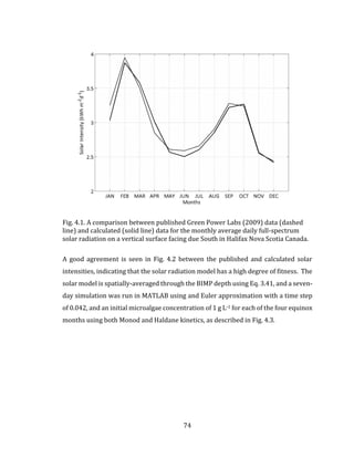
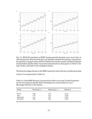
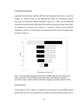
55. 43
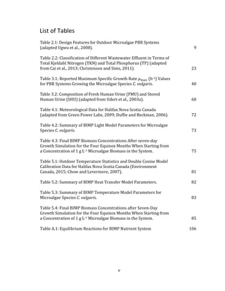
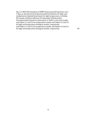
limiting function 𝑓(𝐿 𝑛), the multiplicative growth rate expression given in Eq. 3.17
becomes:
𝜇 = 𝜇 𝑚𝑎𝑥 ∙ ∏ 𝑓(𝐿 𝑛)
𝑛
1
3.18
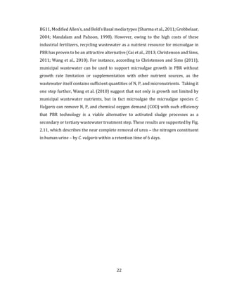
where 𝐿1, 𝐿2, 𝐿3 … 𝐿 𝑛 are specific growth rate limiting functions. For the BIMP system,
four specific growth limiting factors have been described in Chapter 2, including the
availability of sunlight for photosynthesis, the culture temperature as influenced by
both the outdoor and indoor environment, as well as the availability of building
generated nutrient and CO2 resources. Rewriting Eq. 3.18 to include each of these
specific limiting functions yields:
𝜇 = 𝜇 𝑚𝑎𝑥 ∙ 𝑓(𝐼 𝑎𝑣𝑔) ∙ 𝑓(𝑇𝑎𝑣𝑔) ∙ 𝑓 ([𝑆𝑡𝑜𝑡,𝑖] 𝐿
) ∙ 𝑓([𝐶𝑂2] 𝐿) 3.19
As an adaptive method for the design development of the BIMP system, this thesis
will explore the interaction between two limiting factors, such that Eq. 3.19 becomes:
𝜇 = 𝜇 𝑚𝑎𝑥 ∙ 𝑓(𝐼 𝑎𝑣𝑔) ∙ 𝑓(𝑇𝑎𝑣𝑔) 3.20
where 𝐼 𝑎𝑣𝑔 is the average solar radiation incident on the BIMP, and 𝑇𝑎𝑣𝑔 is the average
BIMP culture temperature. The utilization of Monod and Haldane kinetics, and the
application of multiplicative kinetics described by Eq. 3.20 are expanded upon in
Chapters 4 and 5. In the following sections, each of the four limiting functions
described by Eq. 3.19 are described mathematically.
3.5 BIMP Light Dynamics
The modeling of the monthly average hourly sunlight incident on a vertical surface is
well described in the literature (Chwieduk, 2009; Kalogirou, 2009; Duffie and

56. 44
Beckman, 2006), and has been applied to PBR systems in the literature (Pruvost et
al., 2011; Sierra et al., 2008; Grima et al., 1999; Fernandez et al., 1998 ). Typically,
these works utilize the Beer-Lambert approximation to average the incident PAR
through the volume of the PBR culture medium. For instance, Grima et al (1999)
employ a stepwise approach for the averaging the PAR radiation in their continuous
tubular PBR system, which includes the definition of a PAR model and the use of the
Beer-Lambert relationship to describe the spatially averaged PAR amount at any
depth 𝑑 within the PBR culture. To describe light-limited growth within a microalgae
PBR, these authors then couple these light dynamics with an empirically-derived,
photoinhibition growth rate model similar to the Haldane kinetic expression
described in previously in this chapter. Conversely, Pruvost et al., (2011) utilize an
empirically uninhibited Monod type model to describe the biological growth rate
dynamics in their PBR system. According to Bechet et al., (2013), when coupled with
the Beer-Lambert relationship, both Monod and Haldane type expressions have been
used to predict microalgae growth rates for a wide range of light-limited or -inhibited
PBR systems with a high level of accuracy.
For this thesis, it is assumed that the Liu and Jordon (1960) Isotropic Diffuse Sky
Model, as describe by Duffie and Beckman (2006) is sufficiently accurate to describe
the solar resource available for utilization in the BIMP system, despite its
computational ease in relation to more complex solar models (Evseev and Kudish,
2009; Loutzenhiser et al., 2007). It is also assumed that the surface azimuth angle, or
surface tilt deviation from due South, is zero. This is considered optimal for flat-plate
solar collectors in the northern hemisphere (Duffie and Beckman, 2006).
The total monthly average daily incident solar radiation on a horizontal surface 𝐻̅ is
composed of two components, namely the direct beam radiation component, and the
diffuse sky radiation component, such that:
𝐻̅ = 𝐻̅ 𝑏 + 𝐻̅ 𝑑 3.21

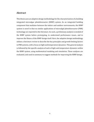
57. 45
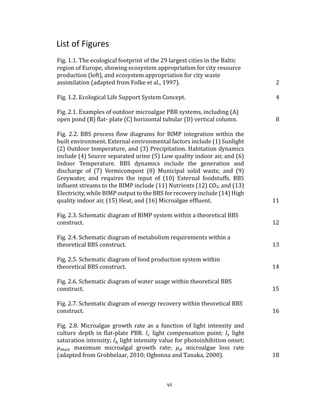
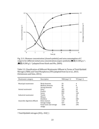
For the monthly average day 𝑁, the total solar intensity 𝐻̅ has been defined
empirically and published for major cities in Canada. To define each of the beam and
diffuse components in Eq. 3.21, a second published empirically defined component is
used. This is the clearness factor 𝐾 𝑡, and it accounts for the attenuation of
extraterrestrial solar radiation as it passes through the atmosphere. Using
empirically derived formulae, the clearness factor can be used to describe the
correlation between the monthly average daily horizontal diffuse sky radiation 𝐻 𝑑
and horizontal total radiation 𝐻 at the surface of the earth:
For 𝜔𝑠 ≤ 81.4o and 0.3 ≤ 𝐾 𝑡 ≤ 0.8:
𝐻 𝑑
𝐻
= 1.391 − 3.560 ∙ 𝐾 𝑡 + 4.189 ∙ 𝐾 𝑡
2
− 2.137 ∙ 𝐾 𝑡
3
3.22
For ωs > 81.4o and 0.3 ≤ 𝐾 𝑡 ≤ 0.8:
𝐻 𝑑
𝐻
= 1.311 − 3.022 ∙ 𝐾 𝑡 + 3.427 ∙ 𝐾 𝑡
2
− 1.821 ∙ 𝐾 𝑡
3
3.23
Here, the criteria for selecting the appropriate empirical correlation is based on
calculating the sunset hour angle 𝜔𝑠 for the average monthly day 𝑁 using the
following relationship:
𝜔𝑠 = 𝑐𝑜𝑠−1(− 𝑡𝑎𝑛 𝜙 ∙ 𝑡𝑎𝑛 𝛿) 3.24
where latitude ϕ = 44.4o for Halifax. The declination angle δ describes the angular
position of the sun at solar noon with respect to the equator, and is calculated as:
𝛿 = 23.45 ∙ 𝑠𝑖𝑛 [
360
365
∙ (284 + 𝑁)] 3.25

58. 46
As the BIMP relies on the diurnal light-dark cycle, the monthly average daily solar
intensity value 𝐻 must be converted to a monthly average hourly value. The monthly
average day length 𝑁 is a description of how many sunlight hours are available
during each monthly average day, and is calculated using the sunset hour angle using
the following equation:
𝐷𝑎𝑦 𝑙𝑒𝑛𝑔𝑡ℎ =
2
15
∙ 𝜔𝑠 = 𝑁 3.26
Dividing the monthly average day length gives an estimation of the number of
sunlight hours before and after local solar time. Then, the specific solar hour angle 𝜔
can be determined for the midpoint of each sunlight hour using:
𝜔 = ±0.25 ∙ (# 𝑜𝑓 𝑚𝑖𝑛𝑢𝑡𝑒𝑠 𝑓𝑟𝑜𝑚 𝑙𝑜𝑐𝑎𝑙 𝑠𝑜𝑙𝑎𝑟 𝑛𝑜𝑜𝑛) 3.27
For example, for January in Halifax, the monthly average day number is 𝑁 = 17, and
by calculating declination δ = −20.92 degrees using Eq. 3.25, the sunset hour angle
is found to be 𝜔𝑠 = 67.78 degrees from Eq. 3.24. The day length is then 𝑁 = 9.04
hours from Eq. 3.26, meaning there are approximately 4.5 hours of sunlight before
and after solar noon. The corresponding specific solar hours are then calculated using
Eq. 3.27 for the midpoint of each solar hour before and after noon.
For each solar hour defined by Eq. 3.26, the monthly average daily solar intensity can
be converted to an hourly solar intensity. This is achieved by defining a ratio 𝑟𝑡, given
as:
𝑟𝑡 =
𝐼
𝐻
3.28

59. 47
where 𝐼 is the average hourly radiation on a horizontal surface (MJ m−2
hr−1
). The
ratio 𝑟𝑡 can be determined for each solar hour using the specific solar hour angle 𝜔
and the sunset hour angle 𝜔𝑠 as follows:
𝑟𝑡 =
𝜋
24
∙ (𝑎 + 𝑏 𝑐𝑜𝑠 𝜔) ∙ (
𝑐𝑜𝑠 𝜔 − 𝑐𝑜𝑠 𝜔𝑠
𝑠𝑖𝑛 𝜔𝑠 −
𝜋𝜔𝑠
180
∙ 𝑐𝑜𝑠 𝜔𝑠
) 3.29
where the coefficients 𝑎 and 𝑏 are given as:
𝑎 = 0.409 + 0.5016 ∙ 𝑠𝑖𝑛(𝜔𝑠 − 60) 3.30
𝑏 = 0.6609 + 0.4767 ∙ 𝑠𝑖𝑛(𝜔𝑠 − 60) 3.31
Similar to Eq. 3.28, an expression for the ratio of hourly total diffuse radiation on a
horizontal surface 𝑟𝑑 is:
𝑟𝑑 =
𝐼 𝑑
𝐻 𝑑
3.32
Where 𝐼 𝑑 is the average hourly diffuse radiation on a horizontal surface (MJ m2 h-1),
and the expression for 𝑟𝑑 is given as:
𝑟𝑑 =
𝜋
24
∙ (
𝑐𝑜𝑠 𝜔 − 𝑐𝑜𝑠 𝜔𝑠
𝑠𝑖𝑛 𝜔𝑠 −
𝜋𝜔𝑠
180
∙ 𝑐𝑜𝑠 𝜔𝑠
) 3.33
Note here that Eq. 3.28 to Eq. 3.33 must be calculated for each solar hour defined by
the day length calculation given in Eq. 3.26, using the specific solar hour angle defined
for that solar hour by Eq. 3.27. Then, for each daily solar hour, and in a manner similar
to that described in Eq. 3.21, the total hourly radiation on a horizontal surface is
expressed using beam 𝐼̅𝑏 and diffuse 𝐼̅𝑑 components as:
𝐼̅ = 𝐼̅𝑏 + 𝐼̅𝑑 3.34

60. 48
For a tilted surface, the hourly beam radiation 𝐼 𝑏,𝑡 diffuse radiation 𝐼 𝑑,𝑡 reflected
radiation 𝐼 𝑟,𝑡 and total radiation 𝐼 𝑡 are estimated through a summation of the beam,
diffuse, and reflected radiation components incident on the surface itself:
𝐼 𝑡 = 𝐼 𝑏,𝑡 + 𝐼 𝑑,𝑡 + 𝐼 𝑟,𝑡 3.35
For the isotropic diffuse sky model, the beam, diffuse, and reflected solar radiation
components in Eq. 4.15 are term-expanded as:
𝐼 𝑡 = 𝐼 𝑏 ∙ 𝑅 𝑏 + 𝐼 𝑑 ∙ (
1 + 𝑐𝑜𝑠 𝛽
2
) + 𝐼 ∙ (
1 − 𝑐𝑜𝑠 𝛽
2
) ∙ 𝜌 𝑔 3.36
where 𝜌 𝑔 is the ground reflectance – or albedo – of the area surrounding the vertical
surface, and 𝛽 = 90°
is the angle of surface tilt. The ratio 𝑅 𝑏 for a tilted surface is
given as:
𝑅 𝑏 =
𝑐𝑜𝑠 𝜃
𝑐𝑜𝑠 𝜃𝑧
=
𝑐𝑜𝑠(𝜙 − 𝛽) ∙ 𝑐𝑜𝑠 𝛿 ∙ 𝑐𝑜𝑠 𝜔 + 𝑠𝑖𝑛(𝜙 − 𝛽) ∙ 𝑠𝑖𝑛 𝛿
𝑐𝑜𝑠 𝜙 ∙ 𝑐𝑜𝑠 𝛿 ∙ 𝑐𝑜𝑠 𝜔 + 𝑠𝑖𝑛 𝜙 ∙ 𝑠𝑖𝑛 𝛿
3.37
Thus, for any calendar day N, Eq. 3.36 can be solved to describe the hourly solar
radiation incident on the vertical exterior surface of the BIMP, for each daily solar
hour defined by Eq. 3.26.
As a photosynthetic organism, microalgae are only able to utilize a specific spectral
range within the incident solar resource. This range, commonly referred to as PAR,
has a spectrum between λ = 400–700 nm (Richmond, 2004). Only the PAR radiation
is useful in the BIMP system to support photosynthesis, so the monthly average
hourly solar radiation incident on the BIMP system described by Eq. 3.36 must be
reduced by the ratio of PAR to full spectrum solar energy. This ratio has been
calculated by Weyer et al., (2010) as 0.458.

61. 49
A second attenuation of the monthly average hourly solar resource is caused by the
BIMP system itself: light incident on the BIMP exterior glazed surface will be reflected
to a certain degree, thereby attenuating the solar resource. Here a simple correlation
is made between the PAR spectrum, and the visible light spectrum, the latter of which
is also λ = 400–700 nm. As such, published data on visible light transmission of
common glazing materials can be used to approximate the PAR transmission through
the exterior BIMP glazing. Average visible light transmittance values for various
glazing products are described by the Canadian Housing and Mortgage Company
(2004) as between 81 – 89% PAR. Based on the PAR and attenuation reductions here
described, the average monthly hourly PAR that has passed through the exterior
BIMP translucent surface and is impingent on the exterior vertical culture surface is:
𝐼𝑖 = 0.458 ∙ 0.89 ∙ 𝐼 𝑡 = 0.408 ∙ 𝐼 𝑡 3.38
In the following section, the average monthly hourly PAR value described in Eq. 3.38
is spatially averaged through the volume of the BIMP culture medium, for the
description of the light-limited growth rate.
3.5.2 Light-Dependent Growth Rate
The characterization of the light-dependent growth rate in the BIMP system is
dependent on the spatially-averaged PAR density 𝐼 𝑎𝑣𝑔, which can be determined by
averaging the incident solar radiation 𝐼𝑖 through the culture depth d of the BIMP
system. This is achieved using a modified form of the Beer-Lambert relationship, as
described by Yun and Park (2003) as:
𝐼(𝑋, 𝑧) = 𝐼𝑖 ∙ exp(−𝑘 𝑚 ∙ 𝑋 𝑎 ∙ 𝑧) 3.39
where 𝐼𝑖 and 𝐼(𝑋, 𝑧) are the radiation intensity at the BIMP interior culture surface
and at any point 𝑧 (m) from the illuminated surface within the culture medium,

62. 50
respectively. The variable 𝑋 describes the microalgae biomass density (g m-3) within
the BIMP, while the parameter 𝑘 𝑚 represents the mass attenuation coefficient of the
culture medium (m2 g-1). For rectangular photobioreactor geometries, Richmond
(2004) integrated the Beer-Lambert expression given in Eq. 3.39 through the culture
depth d to determine the spatially averaged PAR 𝐼 𝑎𝑣𝑔 available within the BIMP:
𝐼 𝑎𝑣𝑔 = ∫
𝐼(𝑋, 𝑧) ∙ 𝑑𝑧
𝑑
𝑑
0
3.40
For the assumption that the BIMP system is completely mixed, and by using
substitution and solving Eq. 3.40, the spatially-averaged PAR density within the BIMP
for photosynthesis 𝐼 𝑎𝑣𝑔 is given as:
𝐼 𝑎𝑣𝑔 = 0.408 ∙ 𝐼 𝑡 ∙
1 − 𝑒𝑥𝑝(−𝑘 𝑚 ∙ 𝑋 𝑎 ∙ 𝑑)
𝑘 𝑚 ∙ 𝑋 𝑎 ∙ 𝑑
3.41
Using Monod kinetics, the spatially-averaged PAR density dependent microalgal
biomass growth rate function 𝑓1(𝐼 𝑎𝑣𝑔) in the BIMP system is given as:
𝑓1(𝐼 𝑎𝑣𝑔) = (
𝐼 𝑎𝑣𝑔
𝐾𝑠 + 𝐼 𝑎𝑣𝑔
) ; 0 ≤ 𝑓1(𝐼 𝑡) ≤ 1 3.42
where 𝐾𝑠 is the half-saturation constant for light-dependent microalgal growth. Here,
𝑓1(𝐼 𝑎𝑣𝑔) is extended using Haldane kinetics to include the effects of light saturation,
or:
𝑓2(𝐼 𝑎𝑣𝑔) =
(
𝐼 𝑎𝑣𝑔
𝐾𝑠 + 𝐼 𝑎𝑣𝑔 +
𝐼 𝑎𝑣𝑔
2
𝐾𝑖 )
; 0 ≤ 𝑓2(𝐼 𝑡) ≤ 1 3.43
where 𝐾𝑖 is the inhibition constant for light-dependent microalgal growth.

63. 51
3.6 BIMP Temperature Dynamics
For outdoor PBR systems, the impact of the geographically specific environment on
the culture temperature has not been extensively modeled in the literature. Gutierrez
et al., (2008) performed a heat balance on a stand-alone, outdoor batch open tank
PBR, and described variation in culture temperature with time as dependent on five
heat transfer mechanisms, which include solar gain, convection, evaporation,
radiation, and conduction. In addition, these authors described the change in PBR
tank body temperature with time, important in their work for the conductive heat
transfer mechanism. Goetz et al., (2011) use a similar approach, but for an outdoor
horizontal continuous flat-plate-type PBR. Here, the authors replace the term
describing conduction between the PBR and the culture medium with a convective
term, as is typical for flow conditions. Bechet et al., (2010) described an outdoor batch
vertical tubular PBR, and assumed there is no temperature gradient between the PBR
material and the culture medium, thereby affording an analysis with only one PBR
system temperature changing with time. For the BIMP system, the indoor building
environment must also be considered in the heat transfer analysis, a condition not
considered in the aforementioned studies, nor in the PBR literature. Published work
on the solar gain through building windows is useful in this analysis, most notably the
work of Chow et al., (2011a, 2011b), who modeled a window system as a solar
thermal heating device.
For the BIMP system, a heat balance is used to describe the temperature change
within the exterior translucent surface. Based on the characteristics of the incident
solar radiation 𝐼̅𝑡 , as well as the average daily outdoor temperature 𝑇𝑜 and the BIMP
culture temperature 𝑇 𝑤, the temperature change in the exterior BIMP surface is given
as:
𝑚1 ∙ 𝐶 𝑝,1 ∙
𝑑𝑇1
𝑑𝑡
= 𝑄𝑠,1 − 𝑄 𝑟,1 − 𝑄 𝑐,1 − 𝑄 𝑘,1 3.44

64. 52
where 𝑇1 is the temperature of the BIMP exterior translucent surface, while 𝑚1 (kg)
and 𝐶 𝑝,1 (J kg-1 K-1) are the mass and heat capacity of that surface, respectively. The
heat transfer mechanism 𝑄𝑠,1 is the total possible heat gain from the sun for a given
geographic location and BIMP orientation, 𝑄 𝑟,1 is the amount of heat radiated as a
loss from the outside BIMP surface to the exterior environment, and 𝑄 𝑐,1 represents
the convective heat transfer from the exterior surface to the outdoor environment.
Because the BIMP operates in a fed-batch mode, the conductive heat transfer
mechanism dominates across the exterior BIMP surface. As such, 𝑄 𝑘,1 represents the
conductive heat transfer through the exterior surface between the outdoor
environment and the BIMP culture medium. Each of these heat transfer mechanisms
is term expanded and described through the following equations:
𝑄𝑠,1 = 𝛼1 ∙ 𝐴1 ∙ 𝐼̅𝑡 3.45
𝑄 𝑟,1 = 𝜀1 ∙ 𝜎 ∙ 𝐴1 ∙ (𝑇1
4
− 𝑇𝑠𝑘𝑦
4
) 3.46
𝑄 𝑐,1 = ℎ 𝑐,1 ∙ 𝐴1 ∙ (𝑇1 − 𝑇𝑜) 3.47
𝑄 𝑘,1 = ℎ 𝑘,1 ∙ 𝐴1 ∙ (𝑇1 − 𝑇 𝑤) 3.48
Here, 𝛼1 (-) and 𝜖1 (-) are the absorptivity and emissivity of the BIMP exterior
translucent surface, respectively, while 𝐴1 (m2) is the illuminated area of that surface.
The Stefan-Boltzmann constant 𝜎 is equal to 5.67037(10)-8 (W m-2 K-4).
The effective sky temperature 𝑇𝑠𝑘𝑦 (K) used to describe radiation from the
atmosphere is expressed empirically as a function of the outdoor temperature 𝑇𝑜
(Duffie and Beckman, 2006), as:
𝑇𝑠𝑘𝑦 = 0.0552 ∙ 𝑇𝑜
1.5
3.49

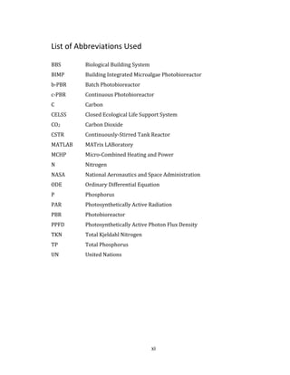
65. 53
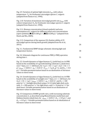
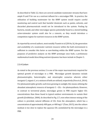
The outdoor temperature 𝑇𝑜 for the average day in any given month is described
statistically for weather stations in Canada using a daily average minimum
temperature 𝑇 𝑚𝑖𝑛, a daily average maximum temperature 𝑇 𝑚𝑎𝑥, and a daily average
temperature 𝑇𝑎𝑣𝑔. To convert the monthly average daily outdoor temperatures to a
monthly average hourly outdoor temperature, the Double Cosine Model as described
by Bilbao et al. (2002) and Chow and Levermore (2007) is used. The Double Cosine
Model provides a method of calculating and linking together the hours of occurrence
of the daily maximum and minimum temperatures using three sinusoidal segments
as given by the following expressions:
For 1 ≤ 𝑡 < 𝑡 𝑇 𝑚𝑖𝑛
:
𝑇𝑜(𝑡) = 𝑇𝑎𝑣𝑔 + 𝑐𝑜𝑠 [
𝜋 ∙ (𝑡 𝑇 𝑚𝑖𝑛
− 𝑡)
24 + 𝑡 𝑇 𝑚𝑖𝑛
− 𝑡 𝑇 𝑚𝑎𝑥
] ∙
𝑇𝑎𝑚𝑝
2
3.50
For 𝑡 𝑇 𝑚𝑖𝑛
≤ 𝑡 ≤ 𝑡 𝑇 𝑚𝑎𝑥
:
𝑇𝑜(𝑡) = 𝑇𝑎𝑣𝑔 + 𝑐𝑜𝑠 [
𝜋 ∙ (𝑡 − 𝑡 𝑇 𝑚𝑖𝑛
)
𝑡 𝑇 𝑚𝑎𝑥
− 𝑡 𝑇 𝑚𝑖𝑛
] ∙
𝑇𝑎𝑚𝑝
2
; 3.51
For 𝑡 𝑇 𝑚𝑎𝑥
< 𝑡 ≤ 24 :
𝑇𝑜(𝑡) = 𝑇𝑎𝑣𝑔 + 𝑐𝑜𝑠 [
𝜋 ∙ (24 + 𝑡 𝑇 𝑚𝑖𝑛
− 𝑡)
24 + 𝑡 𝑇 𝑚𝑖𝑛
− 𝑡 𝑇 𝑚𝑎𝑥
] ∙
𝑇𝑎𝑚𝑝
2
3.52
where 𝑇𝑜(𝑡) is the monthly average hourly outdoor temperature calculated for each
hour 𝑡 between 12:30 am (𝑡 = 1) and 11:30 pm (𝑡 = 24), 𝑡 𝑇 𝑚𝑖𝑛
is the hour of
occurrence of the daily average minimum temperature 𝑇 𝑚𝑖𝑛 , and 𝑡 𝑇 𝑚𝑎𝑥
is the hour of
occurrence of the daily average maximum temperature 𝑇 𝑚𝑎𝑥 . The monthly mean
temperature amplitude 𝑇𝑎𝑚𝑝 is defined as the difference between the monthly
average maximum and minimum temperatures.

66. 54
The convective heat transfer coefficient between the exterior translucent BIMP
surface and the outdoor environment ℎ 𝑐,1 (W m-2 K-1) is a function of the wind speed
𝑉 (m s-1) (Duffie and Beckman, 2006), and is expressed as:
ℎ 𝑐,1 = (5.7 + 3.8 ∙ 𝑉) 3.53
The conductive heat transfer coefficient ℎ 𝑘,1 (W m-2 K-1) through the exterior surface
is expressed as a relationship between the thermal conductivity 𝑘1 (W m-1 K-1) and
depth 𝑑1 (m) of the material (Incropera et al., 2007), or:
ℎ 𝑘,1 =
𝑘1
𝑑1
3.54
Similar to the analysis presented for the exterior BIMP surface but for conditions
characterized by the indoor environment, the change in temperature in the inside
surface of the BIMP can be described using a heat balance based on the indoor
environment, namely the internal temperature 𝑇𝑖. As such, the rate of change in
temperature for the interior translucent BIMP surface is given as:
𝑚2 ∙ 𝐶 𝑝,2 ∙
𝑑𝑇2
𝑑𝑡
= 𝑄𝑠,2 − 𝑄 𝑟,2 − 𝑄 𝑐,2 − 𝑄 𝑘,2 3.55
where 𝑇2 is the temperature of the BIMP interior translucent surface. The heat
transfer mechanism 𝑄𝑠,2 is the total possible heat gain from the sun as transmitted
through both the exterior BIMP surface and the culture medium, 𝑄 𝑟,2 is the amount
of heat radiated from the inside BIMP surface to the indoor environment, and 𝑄 𝑐,2
represents the convective heat transfer from the interior surface to the indoor
environment. And, as for the exterior surface 2 represents the conductive heat
transfer through the interior surface between the outdoor environment and the BIMP
culture medium.

67. 55
Again term expanding these heat transfer mechanism results in the following
equation set:
𝑄𝑠,2 = 𝜏1 ∙ 𝜏 𝑤 ∙ 𝛼2 ∙ 𝐴2 ∙ 𝐼̅𝑡 3.56
𝑄 𝑟,2 = 𝜀2 ∙ 𝜎 ∙ 𝐴2 ∙ (𝑇2
4
− 𝑇𝑠𝑢𝑟
4
) 3.57
𝑄 𝑐,2 = ℎ 𝑐,2 ∙ 𝐴2 ∙ (𝑇2 − 𝑇𝑖) 3.58
𝑄 𝑘,2 = ℎ 𝑘,2 ∙ 𝐴2 ∙ (𝑇2 − 𝑇 𝑤) 3.59
The terms 𝜏1 (-) and 𝜏 𝑤 (-) represent the transmissivity of the exterior BIMP surface
and the culture medium, respectively. The effective indoor surface temperature 𝑇𝑠𝑢𝑟
is assumed equivalent to the indoor temperature 𝑇𝑖 (Chow et al., 2011a, b). The indoor
convective heat transfer coefficient ℎ 𝑐,2 is simply defined as Eq. 3.53 without the wind
speed term (Carlos et al., 2011), or 5.7 W m-2 K-1 when converted to the normal unit
set used in this chapter. As both the interior and exterior BIMP surfaces are the same
material, the conductive heat transfer coefficient ℎ 𝑘,2through the interior BIMP
surface between the culture medium and the indoor environment is defined using Eq.
3.54.
The change in the BIMP culture temperature 𝑇 𝑤 is dependent on the expressions
developed for the change in exterior and interior translucent BIMP surface
temperatures 𝑇1and 𝑇2, respectively, as described by the following heat balance:
𝑚 𝑤 ∙ 𝐶 𝑝𝑤 ∙
𝑑𝑇 𝑤
𝑑𝑡
= 𝑄𝑠,𝑤 − 𝑄 𝑘,1 − 𝑄 𝑘,2 3.60
with the term expansion resulting in the following equation set:
𝑄𝑠,𝑤 = 𝜏1 ∙ 𝛼 𝑤 ∙ 𝐴 𝑤 ∙ 𝐼̅𝑇 3.61

68. 56
In the following section, these heat transfer analyses will be used to determine the
BIMP culture temperature defined by Eq. 3.60.
3.6.1 Temperature-Dependent Growth Rate
The effect that temperature has on the growth rate of microalgae is described by
Quinn et al. (2011) using two expressions that relate culture medium temperature 𝑇 𝑤
to the activity of the ribulose-1,5-bisphosphate carboxylase/oxygenase – or RuBisCo
– enzyme, which catalyzes the preliminary carbon fixation activities in the microalgae
cell. These expressions are:
𝜑 𝑇 = exp (
𝐸 𝑎
𝑅 ∙ 𝑇𝑜𝑝𝑡
−
𝐸 𝑎
𝑅 ∙ 𝑇 𝑤
) 3.62
𝑓(𝑇 𝑤) =
2 ∙ 𝜑 𝑇
1 + (𝜑 𝑇)2
; 0 ≤ 𝑓(𝑇 𝑤) ≤ 1 3.63
where 𝐸 𝑎 (J mol-1) is the activation energy of the RuBisCo enzyme, and 𝑅 (J K-1 mol-1)
is the universal gas constant. The optimal culture temperature 𝑇𝑜𝑝𝑡 (K) is the
temperature at which microalgae growth is ideal and not temperature limited, and
𝑇 𝑤 is the actual culture temperature.
3.7 BIMP Nutrient Dynamics
In this section, a microalgae nutrient resource consisting of human urine and
rainwater is theoretically defined. As described in Fig. 1.1, an urban region has a large
demand on exurban water resources, requiring both freshwater inputs, and large
ecosystem regions for the treatment of wastewater that is generated. Instead, this
section proposes the BIMP system as an in-situ wastewater treatment device, able to
bioregenerate a human urine/wastewater mixture, without the need of an exurban
ecosystem.

69. 57
The BIMP nutrient medium is described as a mixture of stored rainwater collected
from an urban environment as mixed with stored human urine, as provided from a
wastewater source separation system. The influence of nutrients on biomass growth
includes the definition of the chemical composition of a urine-rainwater mixture to
be used as a nutrient feed, the specific uptake of various aqueous chemical species by
microalgae within the BIMP, and the resulting effect on the BIMP system pH.
Rainwater collected from an urban environment changes pH as it passes through the
various stages of harvesting; Despins et al., (2009) describe a range of pH 5.8 for rural
environments, to 8.2 for industrial areas. Also, rainwater in various North American
regions demonstrate different pH values based on various climatic factors, including
proximity to sea spray, heavy industry, and urbanized areas. Here it is assumed that
rainwater entering the catchment area only has aqueous C species present, and other
species such as N and sulfur dioxides absorbed from the atmosphere are neglected.
This assumption is then used as a first approximation for rainwater pH.
Stored human urine differs from fresh human urine in chemical composition, based
mainly on the hydrolysis of urea according to the following reaction (Udert et al.,
2003a, b):
𝑁𝐻2(𝐶𝑂)𝑁𝐻2 + 2𝐻2 𝑂 → 𝑁𝐻3 + 𝑁𝐻4
+
+ 𝐻𝐶𝑂3
−
3.64
The formation of ammonia and bicarbonate in the hydrolyzed urine system causes the
pH to increase, resulting in the formation of various precipitates (Udert et al., 2003a).
These precipitates settle in the urine storage tank, and as such, it is here assumed that
the stored urine utilized within the BIMP is drawn from the supernatant, while settled
precipitates would be collected and utilized elsewhere. It is also assumed that upon
mixing the source-separated urine and rainwater, new precipitates will not form due
to very low concentrations of calcium and magnesium in rainwater (Udert et al.,
2003b), and ammonia in situ will remain so, and not volatilize within the BIMP
system.

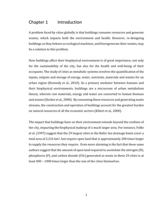
70. 58
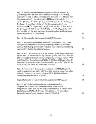
It is assumed that C species in rainwater and urine mix additively to form a new TIC,
whereby the change in pH caused by rainwater dilution – and resulting change in pH
– results in a new equilibrium point, and a new TIC profile after mixing. Also, C species
are not removed from the system based on biological uptake in this study, and instead
the specific species concentrations of TIC are utilized here to calculate changes in the
system pH, based on the nutrient metabolism of microalgae within the BIMP. At any
given time, the TIC profile can be determined based on the system pH here described,
and are utilized as inputs to the BIMP system modeling of aqueous 𝐶𝑂2 uptake by
microalgae, as described in the next section.
All equilibrium constants for the equilibrium equations are for 25 oC, and variations
based on the change in BIMP liquid temperature are neglected. Also, it is assumed that
no complex species exist that have equilibrium dynamics outside those characterized
by the equations in Appendix A.
3.7.1 Rainwater
To determine the pH of rainwater based on the presence of C species, the electro-
neutrality condition must be described. The electro-neutrality expression describes
the balance between the concentrations of C cation and anion species, as well as the
concentrations of hydrogen [𝐻+
] and hydroxyl [𝑂𝐻−
] species present, and is given as
(Stumm and Morgan, 1996):
[𝐻+] = [𝐻𝐶𝑂3
−] + 2 ∙ [𝐶𝑂3
2−] + [𝑂𝐻−
] 3.65
Where concentrations [𝐻+
] and [𝑂𝐻−
] are related by the equilibrium reaction
constant for water 𝐾 𝑊, as provided in Appendix A. To determine the bicarbonate
[𝐻𝐶𝑂3
−] and carbonate [𝐶𝑂3
2−] aqueous concentrations, the equivalent carbonic acid
aqueous concentration [𝐻2 𝐶𝑂3]∗
must first be described.

71. 59
This is achieved using the dynamics of CO2 mass transfer from the gas-phase
(atmosphere) to the liquid phase (rainwater), as expressed by the equilibrium
reaction (England et al., 2011):
[𝐶𝑂2] 𝐺 + 𝐻2 𝑂
𝐻 𝐶
↔ [𝐻2 𝐶𝑂3]∗ 3.66
where 𝐻 𝐶 = 3.4 x 10-2 mol L∙atm-1 is the Henry’s constant for CO2 , the concentration
[𝐶𝑂2] 𝐺 is equivalent to the partial pressure 𝑃𝐶𝑂2
of CO2 in the atmosphere. The
equivalent carbonic acid concentration is the sum of aqueous CO2 and carbonic acid
described by the relationship [𝐻2 𝐶𝑂3]∗
= [𝐶𝑂2] 𝐿 + [𝐻2 𝐶𝑂3] for open freshwater
systems, and is a convention used due to the slow rate of conversion of aqueous CO2
to carbonic acid. Thus, the equilibrium equation describing the equivalent carbonic
acid concentration is given as:
[𝐻2 𝐶𝑂3]∗
= 𝐻 𝐶 ∙ 𝑃𝐶𝑂2 3.67
Then, by expressing the equilibrium equations for bicarbonate and carbonate in
terms of the equivalent carbonic acid concentration, and through substitution, the
expression for electro-neutrality given in Eq. 3.65 becomes:
[𝐻+] =
2 ∙ 𝐾𝐶2 ∙ 𝐾𝐶3 ∙ 𝐻 𝐶 ∙ 𝑃𝐶𝑂2
[𝐻+]2
+
𝐾𝐶2 ∙ 𝐻 𝐶 ∙ 𝑃𝐶𝑂2
[𝐻+]
+
𝐾 𝑊
[𝐻+]
3.68
where, after rearranging, a polynomial equation with respect to [𝐻+] is achieved:
[𝐻+]3
− [𝐻+] ∙ (𝐾𝐶2 ∙ 𝐻 𝐶 ∙ 𝑃𝐶𝑂2
+ 𝐾 𝑊) − 2 ∙ 𝐾𝐶2 ∙ 𝐾𝐶3 ∙ 𝐻 𝐶 ∙ 𝑃𝐶𝑂2
= 0 3.69
For an atmospheric partial pressure 𝑃𝐶𝑂2
= 4 x 10-4 atm (equivalent to a concentration
of [𝐶𝑂2] 𝐺 = 400 ppm), Eq. 3.69 can be solved using the roots function in MATLAB,
yielding a concentration [𝐻+] = 2.476 x 10-6 M, and a corresponding pH = 5.6 for the
rainwater system here considered. This pH value is in the range of rainwater cistern

72. 60
values for Canada (Despins et al., 2009). The total inorganic C (TIC) in the rainwater
system can be described as:
[𝑇𝐼𝐶] = [𝐶𝑂2] 𝐿 + [𝐻2 𝐶𝑂3] + [𝐻𝐶𝑂3
−] + [𝐶𝑂3
2−
] 3.70
where the equilibrium equations for each species in Eq. 3.70 utilize Eq. 69. The
equilibrium equations for rainwater are provided in Appendix A.
3.7.2 Human Urine
Based on the formation of precipitates, as well as the volatilization of ammonia within
the source-separated urine system, the difference between chemical species density
in fresh and stored human urine are described in Table 3.2.
Table 3.2: Composition of Fresh Human Urine (FMU) and Stored Human Urine (SHU)
(adapted from Udert et al., 2003a)
Species Fresh urine Stored urine
Ammonia (g N m-3) 254 1720
Urea (g N m-3) 5810 73
Phosphate (g P m-3) 367 76
Calcium (g m-3) 129 28
Magnesium (g m-3) 77 1
Sodium (g m-3) 2670 837
Potassium (g m-3) 2170 770
Sulphate (g 𝑆𝑂4 m-3) 748 292
Chloride (g m-3) 3830 1400
Carbonate (g C m-3) - 966
Total COD (g 𝑂2 m-3) 8150 1650
pH 7.2 9.0
For the chemical species described in Table 3.2, the relevant equilibrium equations
and reactions for the urine-rainwater system are described in Appendix A. Stored
urine has two important characteristics. First, stored urine is diluted with water, as
part of mechanism used to separate it from solid wastes in a source separation
system. Second, the pH = 9 of the stored urine is suboptimal for C. Vulgaris growth

73. 61
(Mayo, 1997), and therefore must be buffered prior to utilization within the BIMP.
The requirements of electro-neutrality within the BIMP suggest that the
concentration [𝐻+
] – and thus the 𝑝𝐻 – can be described as follows:
[𝑂𝐻−] + [𝐻𝐶𝑂3
−] + 2 ∙ [ 𝐶𝑂3
−2] +[𝐻2 𝑃𝑂4
−
] + 2 ∙ [ 𝐻𝑃𝑂4
−2] + 3 ∙ [ 𝑃𝑂4
−3] + 2 ∙
[𝑆𝑂4
−2] + [𝐶𝑙−] = [𝐻+] + [𝑁𝐻4
+] + 2 ∙ [𝐶𝑎+2] + 2 ∙ [𝑀𝑔+2] + [𝑀𝑔+] +
[𝑁𝑎+] + [𝐾+
]
3.71
3.7.3 Nutrient-Dependent Growth rate
To describe the change in macronutrient concentration in the BIMP system, the yield
coefficient 𝑌𝑆 𝑡𝑜𝑡,𝑖
for each must be defined, as is described in Chapter 3. For each
macronutrient in the BIMP culture medium, the rate of biological nutrient uptake
𝑑[𝑆𝑡𝑜𝑡,𝑖] 𝑋
can be described as follows:
𝑑[𝑆𝑡𝑜𝑡,𝑖] 𝑋
𝑑𝑡
= −𝜇 𝑚𝑎𝑥 ∙ 𝑋 𝑎 ∙ 𝑌𝑆 𝑡𝑜𝑡,𝑖
3.72
The change in macronutrient concentration in the BIMP culture medium can then be
defined as:
𝑑[𝑆𝑡𝑜𝑡,𝑖] 𝐿
𝑑𝑡
= [𝑆𝑡𝑜𝑡,𝑖]𝑖
+
𝑑[𝑆𝑡𝑜𝑡,𝑖] 𝑋
𝑑𝑡
3.73
Using the multiplicative growth kinetics described by Eq. 3.18, the nutrient limitation
function is given as:
𝑓 ([𝑆𝑡𝑜𝑡,𝑖] 𝐿
) = ∏
[𝑆𝑡𝑜𝑡,𝑖] 𝐿
𝐾𝑆 𝑡𝑜𝑡,𝑖
+ [𝑆𝑡𝑜𝑡,𝑖] 𝐿
𝑛
𝑖=1
; 0 ≤ 𝑓 ([𝑆𝑡𝑜𝑡,𝑖] 𝐿
) ≤ 1 3.74

74. 62
3.8 BIMP CO2 Dynamics
This section introduces the mathematical modeling of the dynamics of BIMP CO2
utilization. Here, the model describes the mechanism of bubbling CO2 into the BIMP
at various concentrations, and the corresponding dynamics of mass transfer, and
biological uptake that result. An important consideration in this chapter is the
mechanism by which microalgae fixate aqueous C. To ensure that the biological
models for microalgal uptake of C remain consistent, and an assumption must be
made whether microalgae preferentially uptake a specific aqueous C type. Concas et
al., (2012) assume that C. Vulgaris are indifferent in their selection of aqueous C
species, while Pegallapati and Nirmalakhandan (2012) select bicarbonate [𝐻𝐶𝑂3
−
]
based on the prevalence of the aforementioned species in the pH range of 6.8 – 7.4,
considered ideal for C. Vulgaris.
A secondary consideration here is the dynamics present with the utilization of urban
wastewater – either source separated urine, or secondary and/or tertiary wastewater
effluent – as aqueous C species are more than likely present as a result of urease
degradation of urea, thereby changing again the dynamics of the model. As part of a
comprehensive urban waste strategy, the BIMP is challenged with using said
wastewater, thereby creating a meta-variable set that is rarely discussed and/or
modeled within the literature.
The influence of aqueous CO2 on biomass growth as described in this section includes
the definition CO2 gas-liquid mass transfer from bubbles sparged to the BIMP culture
medium, the dynamics of CO2 hydrolysis, and the specifics of biological uptake of
aqueous CO2 species by microalgae within the BIMP. Also of interest here is the
power required to sparge the CO2 (Hulatt and Thomas, 2011).

75. 63
3.8.1 Biological Phase
The biological uptake of CO2 is similar to that described in Appendix C for nutrients,
or:
𝑑[𝐶𝑂2] 𝐿,𝑋
𝑑𝑡
= −𝜇 𝑚𝑎𝑥 ∙ 𝑋 𝑎 ∙ 𝑌𝑆𝑖/𝐴 3.75
3.8.2 Gas Phase
Gas-liquid mass transfer of CO2 from sparged air to the BIMP microalgal culture
medium is defined by both time and space; the former being a function of the gas
holdup 𝜖 within the BIMP culture, while the latter a function of the BIMP culture
medium height 𝑦. To state this more directly, sparged air entering that enters the
bottom of the BIMP will continuously undergo gas-liquid mass transfer as bubbles
rise through the height of the culture medium, meaning the CO2 concentration within
the bubbles at the base of the BIMP will be greater than the CO2 concentration of the
bubbles entering the BIMP headspace. In general, across the volume of the BIMP
culture medium, the gas-liquid mass transfer rate is defined as:
𝑑[𝐶𝑂2] 𝐺
𝑑𝑡
= 𝐹𝐺 ∙ ([𝐶𝑂2] 𝐺,𝑖 − [𝐶𝑂2] 𝐺,𝑜) 3.76
Where [𝐶𝑂2]𝑖 is the concentration of CO2 in bubbles sparged at the base of the BIMP,
while [𝐶𝑂2] 𝑜 is the concentration of CO2 in sparged bubbles leaving the BIMP culture
medium and entering the headspace. Consider then, a differential volume within the
BIMP, as characterized by the height dimension 𝑑𝑧. The gas-liquid mass transfer 𝐽 𝑑𝑧
for the differential volume 𝑉𝑑𝑧 is described by Chisti (1989) as:
𝐽 𝑑𝑧 = 𝑘 𝐿 𝑎 𝐿 ∙ ([𝐶𝑂2] 𝐿
∗
− [𝐶𝑂2] 𝐿) ∙ 𝑉𝑑𝑧 3.77

76. 64
Where 𝑉𝑑𝑧 = (1 − 𝜖) ∙ 𝐴 ∙ 𝑑𝑧 describes the available aqueous culture medium within
the differential volume for gas-liquid mass transfer. Also, by definition during steady-
state BIMP operation, the rate of gas-liquid mass transfer within the differential
volume 𝑉𝑑𝑧 must be:
𝐽 𝑑𝑧 = 𝐹𝐺 ∙ [𝐶𝑂2] 𝐺,𝑖 − 𝐹𝐺 ∙ ([𝐶𝑂2] 𝐺,𝑖 + 𝑑[𝐶𝑂2] 𝐺,𝑑𝑧) = −𝐹𝐺 ∙ 𝑑[𝐶𝑂2] 𝐺,𝑑𝑧 3.78
Thus, the amount of CO2 transferred from the gaseous phase to the aqueous BIMP
phase within the differential volume can be described by equating Eq. 3.77 with Eq.
78 and rearranging, or:
𝑑[𝐶𝑂2] 𝐺,𝑑𝑧
𝑑𝑧
= 𝑘 𝐿 𝑎 𝐿 ∙ ([𝐶𝑂2] 𝐿
∗
− [𝐶𝑂2] 𝐿) ∙ (1 − 𝜖) ∙
𝐴
𝐹𝐺
3.79
where [𝐶𝑂2] 𝐿
∗
= 𝐻𝑐 ∙ [𝐶𝑂2] 𝐺,𝑑𝑧, for 𝐻𝑐 as the Henry Constant for CO2 between gas and
BIMP culture medium. Eq. 3.79 can is now rearranged and to solve using boundary
conditions characteristic of the BIMP:
∫
𝑑[𝐶𝑂2] 𝑑𝑧
(𝐻𝑐 ∙ [𝐶𝑂2] 𝐺,𝑑𝑧 − [𝐶𝑂2] 𝐿)
[𝐶𝑂2] 𝐺,𝑜
[𝐶𝑂2] 𝐺,𝑖
= −𝑘 𝐿 𝑎 𝐿 ∙ (1 − 𝜖) ∙
𝐴
𝐹𝐺
∙ ∫ 𝑑𝑧
𝑦
𝑜
3.80
Thus, by solving Eq. 3.80 and rearranging yields the concentration of CO2 leaving the
gaseous bubble phase and entering the headspace of the BIMP. Assuming no gas-
liquid mass transfer between the headspace and BIMP culture medium, the amount
of CO2 leaving the BIMP is described as:
[𝐶𝑂2] 𝐺,𝑜 =
1
𝐻𝑐
∙ [((𝐻𝑐 ∙ [𝐶𝑂2] 𝐺,𝑖 − [𝐶𝑂2] 𝐿) ∙ exp (
(𝑘 𝐿 𝑎 𝐿 ∙ (1 − 𝜖) ∙ 𝐴 ∙ 𝑦
𝐹𝐺
))
+ [𝐶𝑂2] 𝐿]
3.81

77. 65
Returning then to Eq. 3.76, the rate of CO2 transferred from the sparged gas phase to
the liquid phase within the BIMP is:
𝑑[𝐶𝑂2] 𝐺
𝑑𝑡
= 𝐹𝐺 ∙ [[𝐶𝑂2] 𝐺,𝑖 −
1
𝐻𝑐
∙ [((𝐻𝑐 ∙ [𝐶𝑂2] 𝐺,𝑖 − [𝐶𝑂2] 𝐿) ∙ exp (
(𝑘 𝐿 𝑎 𝐿 ∙ (1 − 𝜖) ∙ 𝐴 ∙ 𝑦
𝐹𝐺
))
+ [𝐶𝑂2] 𝐿]]
3.82
By design, the BIMP behaves as a pneumatically-agitated bubble column reactor with
a rectangular shape factor. For this type of reactor, Acien-Fernandez et al., (2012)
present empirical relationships describing both the mass transfer coefficient 𝑘 𝐿 𝑎 𝐿
and gas holdup 𝜖, as dependent on the power input through gas sparging per unit
reactor culture medium volume:
𝑘 𝐿 𝑎 𝐿 = 2.39(10)−4
∙ (
𝑃𝐺
𝑉𝐿
)
0.86
3.83
𝜖 = 3.32(10)−4
∙ (
𝑃𝐺
𝑉𝐿
)
0.97
3.84
The power input per volume factor 𝑃𝐺 𝑉𝐿⁄ is a function of the superficial gas velocity
in the aerated zone of the reactor, the density of the reactor culture medium, and
gravitational acceleration:
𝑃𝐺
𝑉𝐿
= 𝜌 𝐿 ∙ 𝑔 ∙ 𝑈 𝐺 3.85

78. 66
Where the superficial gas velocity 𝑈 𝐺 is defined as the flow rate of aeration gas per
area of aeration zone, or:
𝑈 𝐺 =
𝑄 𝐺
𝐴 𝐺
3.86
3.8.3 Liquid Phase
If it is assumed that C. Vulgaris preferentially uptake aqueous CO2 then the amount of
C in that form available for photosynthesis may limit growth, based on the dynamics
of CO2 hydrolysis with respect to pH within the BIMP culture medium. For the
hydrolysis of CO2 the following overall chemical equilibria equations (England et al.,
2011) are considered.
[𝐶𝑂2] 𝐿 + 𝐻2 𝑂
𝐾𝑐1
↔ 𝐻2 𝐶𝑂3
3.87
𝐻2 𝐶𝑂3
𝐾𝑐2
↔ 𝐻𝐶𝑂3
−
+ 𝐻+ 3.88
𝐻𝐶𝑂3
−
𝐾𝑐3
↔ 𝐻+
+ 𝐶𝑂3
−2 3.89
Here, the variables 𝐾𝑖 (for 𝑖 =C1, C2, C3) represent the equilibrium constant for each
reaction, respectively. These equilibrium constants are related to the reaction rates
for each CO2 hydrolysis reaction by the relationship proposed by Erickson et al.,
(1987):
𝐾𝑐𝑖 =
𝑘+𝑖
𝑘−𝑖
3.90
where 𝑘+𝑖 represents the forward reaction rate of the 𝑖th reaction, while 𝑘−𝑖
represents the reverse reaction rate of the 𝑖th reaction. Along with the characteristics
of biological uptake of [𝐶𝑂2] 𝐿 in situ, the reaction rates 𝑘±𝑖 are utilized with respect

79. 67
to the dynamic concentration of each C species within the BIMP to determine the
availability of [𝐶𝑂2] 𝐿 for microalgal photosynthesis. This is described as:
𝑉𝐿 ∙
𝑑[𝐶𝑂2] 𝐿
𝑑𝑡
=
𝑑[𝐶𝑂2] 𝐺
𝑑𝑡
+
𝑑[𝐶𝑂2] 𝐿,𝑋
𝑑𝑡
+ [𝐶𝑂2] 𝐿,𝑖 + 𝑘−1 ∙ [𝐻2 𝐶𝑂3] − 𝑘1
∙ [𝐶𝑂2] 𝐿
3.91
The rate of change of concentration for each C species – those not [𝐶𝑂2] 𝐿 – are
dependent on the kinetics of Eq. 3.91, as well as the initial concentration of each
species present as a result of utilizing a urine-rainwater mixture as the BIMP
nutrient source. These concentrations are therefore given as:
𝑉𝐿 ∙
𝑑[𝐻2 𝐶𝑂3]
𝑑𝑡
= [𝐻2 𝐶𝑂3]𝑖 + 𝑘1 ∙ [𝐶𝑂2] 𝐿 + 𝑘−2 ∙ [𝐻+] ∙ [𝐻𝐶𝑂3
−
] − 𝑘−1
∙ [𝐻2 𝐶𝑂3] − 𝑘2 ∙ [𝐻2 𝐶𝑂3]
3.92
𝑉𝐿 ∙
𝑑[𝐻𝐶𝑂3
−]
𝑑𝑡
= [𝐻𝐶𝑂3
−]𝑖 + 𝑘2 ∙ [𝐻2 𝐶𝑂3] + 𝑘−3 ∙ [𝐻+] ∙ [𝐶𝑂3
−2] − 𝑘−2 ∙ [𝐻+]
∙ [𝐻𝐶𝑂3
−] − 𝑘3 ∙ [𝐻𝐶𝑂3
−]
3.93
𝑉𝐿 ∙
𝑑[𝐶𝑂3
−2]
𝑑𝑡
= [𝐶𝑂3
−2]𝑖 + 𝑘3 ∙ [𝐻𝐶𝑂3
−] − 𝑘−3 ∙ [𝐻+] ∙ [𝐶𝑂3
−2] 3.94
where [𝐻+
] is defined based on the nutrient chemical equilibria and electro-
neutrality requirements for the BIMP nutrient media and microalgal uptake dynamics
presented in Appendix A.

80. 68
3.8.4 CO2-Dependent Growth Rate
Using the Monod growth kinetics described in Chapter 3, the CO2 limitation function
is given as:
𝑓([𝐶𝑂2] 𝐿) =
[𝐶𝑂2] 𝐿
𝐾𝑐 + [𝐶𝑂2] 𝐿
; 0 ≤ 𝑓([𝐶𝑂2] 𝐿) ≤ 1 3.95
3.9 Discussion
This chapter introduces the b-PBR dynamic modeling method, where the microalgae
biomass concentration 𝑋 𝑎 is shown to be dependent on a specific growth rate 𝜇, for
which two kinetic expressions are described, including the uninhibited Monod
growth rate and the inhibited Haldane growth rate. For the former of these
expressions, the depletion of a single substrate 𝑆𝑖 in a b-PBR system is shown to limit
the growth of the microalgae, as described in Fig. 3.3. This analysis is extended to the
specific case of sunlight as substrate, which is not exhausted with the b-PBR, but
instead varies diurnally, resulting in a sawtooth microalgae growth dynamic, as
described in Fig. 3.4. As was described in Chapter 2, the sunlight intensity may be such
that it limits growth through photoinhibition, a concept introduced using a
comparison between the Monod and Haldane growth rates as described in Fig. 3.5. A
brief review of the empirical derivation of the maximum specific growth rate 𝜇 𝑚𝑎𝑥
was presented. As described in Table 3.1, there exists a large variance in the literature
for values of 𝜇 𝑚𝑎𝑥 , even in systems using the same microalgae species. This is a
consequence of the individual PBR system dynamics that are present in these studies,
and as such, this thesis will utilize a sensitivity analysis in the modeling
characterization of the BIMP system.
The analysis of the growth rate for a single-limiting substrate is extended to the case
of multiple-limitation dynamics, where two or more substrate 𝑆1, 𝑆2, 𝑆3, … , 𝑆 𝑛 can co-
limit growth, as described using the multiplicative growth rate. For the scenario of

81. 69
two co-limiting substrates 𝑆1 and 𝑆2 , the multiplicative growth rate is describe in Fig.
3.6. The multiplicative growth rate expression is then generalized in terms of a
specific limiting function 𝑓(𝐿 𝑛) , and applied to the BIMP system by defining four
unique limiting functions, one each for sunlight 𝑓(𝐼 𝑎𝑣𝑔), culture temperature 𝑓(𝑇𝑎𝑣𝑔),
nutrients 𝑓 ([𝑆𝑡𝑜𝑡,𝑖] 𝐿
), and CO2 [𝐶𝑂2] 𝐿. The analysis of a single limiting function
𝑓(𝐼 𝑎𝑣𝑔) on the growth dynamic in the BIMP system is the subject of Chapter 4. The
analysis of BIMP system multiplicative growth kinetics 𝑓(𝐼 𝑎𝑣𝑔) ∙ 𝑓(𝑇𝑎𝑣𝑔) is the
subject of Chapter 5.

82. 70
Chapter 4 Modeling Light Dynamics in a BIMP System
4.1 Introduction
As described in Chapter 2, microalgae grown in PBR systems have specific light
requirements that must be maintained to ensure photosynthesis is not limited or
inhibited. As such, this chapter presents an analysis of the single-limitation growth
dynamics in the BIMP system, as defined by the available outdoor PPFD resource.
4.2 System Description
The influence of light on biomass growth as described in this chapter includes the
definition of the total monthly average daily solar resource incident on a horizontal
terrestrial surface, and the conversion of this to a monthly average hourly vertical
solar resource 𝐼 𝑡. As stated in Chapter 3, the influence of indoor light on the BIMP
system is neglected. The hourly solar radiation is then reduced by two mechanistic
principles: the first reduction is to quantify the PPFD value that could be utilized by
microalgae for photosynthesis; the second reduction is a result of reflecting a small
portion of the PPFD from the exterior vertical translucent material surface of the
BIMP system. These considerations and the BIMP system analyzed in this section are
presented in Fig 4.1.
The average PPFD available for photosynthesis 𝐼 𝑎𝑣𝑔 at any depth 𝑑 within the BIMP
system is determined using the Beer-Lambert relationship, which is spatially
averaged throughout the rectangular culture profile. Here it is assumed that the BIMP
has an illuminated culture surface area of 1 m2. Finally the biological utilization of
light by microalgae in the BIMP system is described using two kinetic theories for
growth.

83. 71
Fig. 4.1. Schematic for light interaction in BIMP system.
4.3 Mathematical Model
Using Eq. 3.12 in Chapter 3 with the specific light-growth rate function, the biomass
growth rate for the light-limited BIMP system can be calculated using:
𝑑𝑋 𝑎
𝑑𝑡
= [𝜇 𝑚𝑎𝑥 ∙ 𝑓𝑖(𝐼 𝑎𝑣𝑔) − 𝜇 𝑑] ∙ 𝑋 𝑎 4.1
where 𝐼 𝑎𝑣𝑔 is the spatially-averaged PPFD in the BIMP system, as defined in Chapter
3 for both Monod and Haldane kinetics. The following section describes the model
inputs, including any assumptions that are made. The model is based on the
theoretical cultivation of the microalgae species C. vulgaris.

84. 72
4.3.1 Solar model
For the determination of incident solar radiation on a vertical surface in Halifax,
published meteorological data, as described in Table 4.1, are here utilized.
Table 4.1: Meteorological Data for Halifax Nova Scotia Canada (adapted from Green
Power Labs, 2009; Duffie and Beckman, 2006).
Jan Feb Mar Apr May Jun Jul Aug Sep Oct Nov Dec
𝑁 17 47 75 105 135 162 198 228 258 288 318 344
𝐻̅ 5.58 8.78 12.64 15.52 18.07 19.98 19.73 17.57 14.33 9.65 5.69 4.54
𝐾 𝑡
0.41 0.46 0.48 0.44 0.44 0.48 0.47 0.50 0.50 0.45 0.39 0.35
𝜌 𝑔 0.70 0.70 0.40 0.30 0.20 0.20 0.20 0.20 0.20 0.30 0.40 0.70
The assumed ground reflectance values presented in Table 4.1 are based on those
found in the literature corresponding to winter months with high reflectance due to
snow cover, and summer months with low reflectance due to vegetation and
absorptive materials such as asphalt. For the purposes of the analysis presented in
the Results section, the dynamics of light-growth in the BIMP system will be
simulated for the four equinox months of March, June, September, and December. It
is assumed that these four months will be sufficient to characterize light in the BIMP
system.
4.3.2 Biological model
The growth of microalgae in the BIMP system is assumed to follow batch dynamics,
as described by Eq. 3.12 in the previous chapter. The specific biological parameters
for C. vulgaris that are used in the simulation efforts here presented are summarized
in Table 4.2.

85. 73
Table 4.2: Summary of BIMP Light Model Parameters for Microalgae Species C.
vulgaris.
Parameter Nomenclature Value Unit Reference
Mass attenuation coefficient 𝑘 𝑚 0.334 m2 g-1 Huesemann et al., (2013)
Culture depth 𝑑 0.05 m Hu et al., (1996)
Half-saturation constant 𝐾𝑠 15.90 µmol m-2 s-1 Yun and Park, (2003)
Light inhibition constant 𝐾𝑖 200 µmol m-2 s-1 Kumar et al., (2011)
Maximum growth rate 𝜇 𝑚𝑎𝑥 0.07 h-1 Huisman et al., (2002)
Microalgae loss rate 𝜇 𝑑 0.006 h-1 Concas et al., (2012)
As was described in Chapter 3, a great deal of variation exists in the literature for the
values presented in Table 4.1. An effort has been made to use median or common
values from the literature, and a sensitivity analysis in the following section was used
to determine the validity of this parameterization. For the purposes of the modeling
study, it is assumed that the microalgae are well mixed and uniformly distributed
throughout the BIMP culture, that there are no other limitation mechanisms in the
BIMP system other than light, and that the physical characteristics of the C. vulgaris
do not change during the length of the simulation.
4.4 Results
To validate the solar model, the following comparison between reported values for
the monthly average daily solar radiation on vertical surface in Halifax (Green Power
Labs, 2009) to that calculated by the solar model presented in this chapter is made.
The comparison was achieved by summing the monthly average hourly values
calculated, and converting to the same unit set as was used in the published work.
These results are presented in Fig. 4.2.

86. 74
Fig. 4.1. A comparison between published Green Power Labs (2009) data (dashed
line) and calculated (solid line) data for the monthly average daily full-spectrum
solar radiation on a vertical surface facing due South in Halifax Nova Scotia Canada.
A good agreement is seen in Fig. 4.2 between the published and calculated solar
intensities, indicating that the solar radiation model has a high degree of fitness. The
solar model is spatially-averaged through the BIMP depth using Eq. 3.41, and a seven-
day simulation was run in MATLAB using and Euler approximation with a time step
of 0.042, and an initial microalgae concentration of 1 g L-1 for each of the four equinox
months using both Monod and Haldane kinetics, as described in Fig. 4.3.

87. 75
Fig. 4.3. MATLAB simulation of BIMP biomass growth dynamics over seven days as
characterized by Monod (solid line) and Haldane (dashed line) kinetic expressions,
for spatially-averaged culture PPFD in Halifax Nova Scotia Canada. (A) March (B) June
(C) September (D) December. Parameterization based on values given in Table 4.1 for
solar model, and Table 4.2 for biological models.
The final microalgae density in the BIMP system for each of the four months described
in Fig. 4.3 is summarized in Table 4.3.
Table 4.3: Final BIMP Biomass Concentrations After seven-day Growth Simulation
for the Four Equinox Months When Starting from a Concentration of 1 g L-1
Microalgae Biomass in the System.
Month Monod (g L-1) Haldane (g L-1) Reduction
March 4.40 4.12 -6.7%
June 3.79 3.67 -3.2%
September 4.11 3.87 -5.8%
December 3.05 2.86 -6.2%

88. 76
4.5 Sensitivity Analysis
A graphical method (Frey and Patil, 2002) is here employed to perform a sensitivity
analysis on selected inputs to the light-growth model. The sensitivity analysis
increased and decreased Monod parameter values by ± 20%, and the MATLAB
simulation was performed to determine the biomass concentration after seven-days,
as compared to a normal value of 4.40 g L-1, as given in Table 4.3 for the Monod
simulation in March. A tornado plot was then generated from these tabulated data,
as shown in Fig. 4.4.
Fig. 4.4. Tornado plot showing the sensitivity of BIMP light-growth model inputs
when varied by ± 20% of their nominal value. Hatch bar indicates change in
parameter value of -20%. Solid bar indicates change in parameter value of +20%.
4.6 Discussion
As described in Fig. 4.3, there is a relatively small reduction in overall BIMP culture
density after the seven-day simulation as a result of using the Haldane expression to

89. 77
account for photoinhibition. This is due to two separate but coupled conditions. First,
Halifax has a comparatively low solar intensity as compared to the average PPFD
reported in Chapter 2 that reaches a horizontal surface. Second, when the horizontal
solar resource is converted to a vertical solar resource, this PPFD is again reduced.
The modest reduction in overall microalgae density that results from using the
Haldane kinetics is in good agreement with the work of Cuaresma et al., (2011), who
suggest that photoinhibition is rarely seen in a vertical flat-plate-type PBR, even in
regions where the PPFD is much greater than Halifax. For an initial microalgae
concentration of 1 g L-1, the BIMP system here described is able to increase the density
to at least 3 g L-1 at the end of the seven-day simulation for each of the four months
described here. These data are in good agreement with the work of Quinn et al (2011),
whose modeling efforts are based on empirical data collected from an industrial PBR
system, and describe a similar increase in microalgae density over the same time
period. This suggests that the BIMP system will not be light limited during the
daytime in the Halifax region, and will have a biomass productivity consistent with
the literature.
The sensitivity of the parameters described in Fig. 4.4 and used in light-growth
modeling also support this preliminary conclusion, as a change of ± 20% does not
dramatically decrease the overall growth potential of the BIMP system. The outlier to
this statement is the maximum growth rate, which is shown to have the most
significant impact as a parameter on the light-growth dynamics in the BIMP system.
To improve the confidence in the parameterization of the maximum growth rate for
the BIMP system, laboratory experiments where C. vulgaris populations are grown as
a function of time under solar conditions similar to those here presented are required.
Perhaps the most interesting outcome of the sensitivity analysis is the increase in
overall productivity of the BIMP system when the culture depth 𝑑 is decreased. A
reduction in cultural depth by definition must increase the spatially averaged PPFD
using the Beer-Lambert expression, creating greater availability of photons for

90. 78
microalgae photosynthesis. This result, along with other considerations from this
chapter, will be discussed in greater detail in Chapter 6.

91. 79
Chapter 5 Modeling Temperature Dynamics in a BIMP
System
5.1 Introduction
In addition to light, photoautotrophic organism survival and growth is strongly
dependent on the temperature of the ecological system which they inhabit. For
microalgae grown in a BIMP system, this habitat is the enclosed aqueous culture
medium, which is subject to both outdoor and indoor environmental factors. As such,
this chapter presents an analysis of the multiplicative growth dynamics in a BIMP
system, as defined by the culture temperature and the availability of light.
5.2 System Description
The influence of temperature on biomass growth as described in this chapter includes
the definition of the amount of solar radiation incident on the exterior surface of the
BIMP, the mechanism of heat transfer resulting from this solar resource passing
through each material phase of the BIMP assembly, and the resulting temperature
profile within. Concurrently, the influence of the outdoor and indoor ambient
temperatures on transient heat transfer mechanisms to and from the BIMP system
are described. A schematic showing these heat transfer mechanisms as they relate to
the BIMP system is described in Fig. 5.1.
Several assumptions are made with respect to the formulation of the temperature-
growth model presented in this chapter. First, it is assumed that the BIMP operates
in a fed-batch mode with an illuminated culture surface area of 1 m2, with both the
interior and exterior BIMP translucent surfaces constructed of the same material.
The BIMP culture medium is assumed to be completely mixed, with all physical
properties, including temperature, considered to be uniform.

92. 80
Fig. 5.1 Schematic for temperature interaction in the BIMP system
Additionally, as microalgal density and nutrient concentration in the BIMP are
generally low (of the order 1 g L-1), the culture medium thermophysical properties
are considered equivalent to those of water at standard temperature and pressure.
The BIMP headspace is assumed to be at the same temperature as the culture
medium, and saturated with water. There is therefore no evaporative heat transfer
from the top surface of the BIMP culture medium to the headspace. The temperature
across the outside and inside translucent surfaces are assumed constant throughout
the material, and thus the material temperature gradient is neglected. Additionally,
the heat gain in the culture medium caused by microalgal metabolism is neglected.
Finally, the fraction of solar radiation converted into algal biomass during
photosynthesis is assumed constant and equal to 2.5% of the full spectrum incident
solar radiation (Bechet et al., 2010).

93. 81
5.3 Mathematical Model
Using Eq. 3.12 in Chapter 3 with the multiplicative growth rate function given in Eq.
3.20, the biomass growth rate for the light and temperature limited BIMP system can
be calculated using:
𝑑𝑋 𝑎
𝑑𝑡
= [𝜇 𝑚𝑎𝑥 ∙ 𝑓(𝐼̅𝑎𝑣𝑔) ∙ 𝑓(𝑇 𝑤) − 𝜇 𝑑] ∙ 𝑋 𝑎 5.1
where 𝐼 𝑎𝑣𝑔 and 𝑇 𝑤 are the spatially-averaged PPFD and BIMP culture temperature,
respectively, as defined in Chapter 3. The following section describes the model
inputs, including any assumptions that are made. The model is based on the
theoretical cultivation of the microalgae species C. vulgaris.
5.3.1 Temperature model
The data described in Table 5.1 are used for the determination of the outdoor
temperature and wind speed in Halifax.
Table 5.1: Outdoor Temperature Statistics and Double Cosine Model Calibration
Data for Halifax Nova Scotia Canada (Environment Canada, 2015; Chow and
Levermore, 2007).
Month N 𝑇 𝑚𝑖𝑛 (oC) 𝑡 𝑇 𝑚𝑖𝑛
𝑇 𝑚𝑎𝑥 (oC) 𝑡 𝑇 𝑚𝑎𝑥
𝑇𝑎𝑚𝑝 (oC) Wind (m s-1)
January 17 -8.2 14 -0.1 6 8.1 6.3
February 47 -7.5 14 0.4 6 7.9 6.2
March 75 -3.9 14 3.6 5 7.5 6.1
April 105 1.0 15 8.7 5 7.7 5.6
May 135 5.8 15 14.4 4 8.6 5.0
June 162 10.7 16 19.6 4 8.9 5.0
July 198 14.4 15 23.1 4 8.7 4.4
August 228 15.1 15 23.1 5 8.0 4.2
September 258 11.8 15 19.3 5 7.5 4.5
October 288 6.4 14 13.4 6 7.0 5.3
November 318 1.5 14 8.1 6 6.6 6.2
December 344 -4.3 14 2.8 7 7.1 6.4

94. 82
From the data presented in Table 5.1, an average wind speed of 5.3 m s-1 is assumed.
The BIMP interior and exterior surface are assumed to be equivalent, and to have
thermophysical properties akin to glass. For a depth of 6 mm, the glass interior and
exterior BIMP surface is assumed to have a mass of 14 kg (Duffie and Beckman, 2006).
The BIMP culture medium is assumed to have a depth of 0.05 m. The outdoor
temperature is variable throughout the day, as described in Eq. 3.50-3.52, meaning
that the effective sky temperature 𝑇𝑠𝑘𝑦 will also be variable, as per Eq. 3.49. Table 5.2
presents the numerical values for the parameters used in the temperature model.
Table 5.2: Summary of BIMP Heat Transfer Model Parameters.
Parameter Nomenclature Value Unit Reference
Thickness of glass 𝑑1, 𝑑2 0.006 m (-)
Mass of glass 𝑚1, 𝑚2 14 kg Duffie and Beckman, (2006)
Heat capacity of glass 𝐶 𝑝,1, 𝐶 𝑝,2 750 J kg-1 K-1 Incropera et al., (2007)
Conductivity of glass 𝑘1, 𝑘2 1.4 W m-1 K-1 Incropera et al., (2007)
Absorptivity of glass 𝛼1, 𝛼2 0.05 (-) Goetz et al., (2011)
Emissivity of glass 𝜀1, 𝜀1 0.92 (-) Goetz et al., (2011)
Transmissivity of glass 𝜏1, 𝜏2 0.95 (-) Goetz et al., (2011)
Thickness of water 𝑑 𝑤 0.05 m (-)
Mass of water 𝑚 𝑤 50 kg (-)
Heat capacity of water 𝐶 𝑝,𝑤 4180 J kg-1 K-1 Goetz et al., (2011)
Absorptivity of water 𝛼 𝑤 0.90 (-) Goetz et al., (2011)
Transmissivity of water 𝜏 𝑤 0.10 (-) Bechet et al., 2010)
Wind velocity 𝑉 5.43 m s-1 Table 5.1
Indoor temperature 𝑇𝑖, 𝑇𝑠𝑢𝑟 294 K (-)
Outdoor conv. coefficient ℎ 𝑐,1 26.35 W m-2 K-1 Eq. 5.9
Indoor conv. coefficient ℎ 𝑐,2 5.7 W m-2 K-1 Carlos et al., (2011)
Conduction coefficient ℎ 𝑘,1, ℎ 𝑘,2 233.33 W m-2 K-1 Eq. 510
For the purposes of the analysis presented in the Results section, the dynamics of
temperature-growth in the BIMP system were simulated for the four equinox months
of March, June, September, and December. It is assumed that these four months are
sufficient to characterize temperature in the BIMP system.

95. 83
5.3.2 Biological model
The growth of microalgae in the BIMP system is assumed to follow batch dynamics,
as described by Eq. 3.12. The specific biological parameters for C. vulgaris that were
used in the simulation are summarized in Table 5.3. It is assumed that the physical
characteristics of C. vulgaris described in Table 5.3 do not change during the length
of the simulation.
Table 5.3: Summary of BIMP Temperature Model Parameters for Microalgae Species
C. vulgaris.
Parameter Nomenclature Value Unit Reference
Activation energy 𝐸 𝑎 62.5 kJ mol-1 Cen and Sage, (2005)
Gas constant 𝑅 8.314 J K-1 mol-1 (-)
Optimal temperature 𝑇𝑜𝑝𝑡 305.4 K Mayo, (1997)
5.4 Results
The variation in daily temperature for each of the four months here considered is
based on data for average outdoor conditions in Halifax over an approximately 30-
year time span. The daily variations in outdoor temperature calculated from Eq. 3.50-
3.52 for the equinox months are presented in Fig. 5.2. These data represent the initial
system temperature, and the hourly outdoor temperatures used in the analysis of the
BIMP temperature dynamics. The temperature change in the indoor and outdoor
BIMP surface temperatures, as well as the BIMP culture temperature that occur
during this diurnal temperature variation are also presented in Fig. 5.2.

96. 84
Fig. 5.2. MATLAB simulation of daily variation in outdoor temperature (dashed line)
and the resultant BIMP culture temperature (solid line) for the four equinox months
in Halifax Nova Scotia Canada. (A) March (B) June (C) September (D) December.
Parameterization based on values given in Table 5.2
These temperature dynamics were used in a seven-day simulation was run in
MATLAB using and Euler approximation with a time step of 0.042, and an initial
microalgae concentration of 1 g L-1 for each of the four equinox months with the
multiplicative growth dynamics described by Eq. 5.21. An initial system temperature
for all months is assumed to be equal to the indoor temperature, or 294 K. These
results are compared to the growth dynamics achieved using Monod kinetics in
Chapter 4, and are presented in Fig. 5.3.

97. 85
Fig. 5.3. MATLAB simulation of BIMP biomass growth dynamics over 7 days as
characterized by Monod (solid line) kinetics for light, and multiplicative (dashed
line) kinetic for light-temperature, in Halifax NS Canada. (A) March (B) June (C)
September (D) December. Parameterization based on values given in Table 4.1 for
solar model, and Tables 5.1 and 5.2 for temperature model, and Tables 4.2 and 5.3
for light and temperature biological models, respectively.
The final microalgae density in the BIMP system for each of the four months described
in Fig. 5.3 is summarized in Table 5.4.
Table 5.4: Final BIMP Biomass Concentrations after Seven-Day Growth Simulation
for the Four Equinox Months When Starting from a Concentration of 1 g L-1
Microalgae Biomass in the System.
Month Monod (g L-1) Multiplicative (g L-1) Reduction
March 4.40 2.20 -50.0%
June 3.79 2.42 -36.1%
September 4.11 2.58 -37.2%
December 3.05 1.55 -49.2%

98. 86
5.5 Sensitivity Analysis
The most significant new parameter with a high level of sensitivity presented in this
chapter is the optimal growth temperature of the microalgae species, or 𝑇𝑜𝑝𝑡 as
described in Table 5.3. Here, this value has been parameterized based on published
data for the C. vulgaris species. However, if this value were to be lowered from its
current value of 32.4 0C to 25 oC, the biomass output in September would be equal to
3.87 g L-1 after seven-days of growth, or at the industry standard of 3 g L-1 for growth
in outdoor PBR systems during the same time span.
5.6 Discussion
Apparent from Fig. 5.3 is the damped growth dynamic of the temperature-light
multiplicative growth kinetic as compared with the Monod analysis completed in the
previous chapter. Counterintuitively, this drastic reduction in overall biomass yield
after the seven-day simulation is not a result of too much heat in the system, but
instead not enough. As described in Fig. 5.2, the diurnal increase in BIMP system
temperature lags behind the increase in outdoor temperature, as would be expected.
However, the BIMP system does not increase in temperature, even during the
summer months, in any appreciable manner. This is a consequence of three system
factors. First, the empirical relationships used to estimate the diurnal change in the
hourly outdoor temperature value may underestimate the actual conditions. For
instance, the model predicts for September (𝑁 = 258) a maximum daily temperature
of 19.3 oC, whereas a simple survey of recent Environment Canada would suggest an
average maximum daily temperature at least 3 oC warmer for the same September
day of year. Secondly, variations in the indoor diurnal temperature profile are not
considered at all, and instead a constant indoor temperature of 21 oC is assumed to
be continuously maintained. However, to model the indoor temperature more
accurately, a specific architectural scenario would have to be considered, which is
outside the scope of this thesis.

99. 87
The third factor affecting the temperature profile in Fig. 5.2 is a consequence of
parameterizing the thermophysical properties of the system as akin to a window
system, not a solar thermal device. However, such a parameterization is important to
the adaptive design methodology used in this thesis, and will be discussed in more
detail in Chapter 6. Of additional interest in the analysis presented in Chapter 6 is the
improvement in overall biomass yield with a reduction in the optimal growth
temperature described in Table 5.3.

100. 88
Chapter 6 Conclusions
The work presented in this thesis toward the characterization of a building-
integrated microalgae bioreactor (BIMP) system lends itself to several conclusions
that can be used in an adaptive methodology. These conclusions are summarized in
this chapter.
In Chapter 1, it was shown that urban regions require large extra-urban ecosystems
both for the delivery of consumable materials, and for the discharge of waste
generated through this consumption. This thesis investigated whether buildings can
be designed as part of a larger urban metabolism theory, wherein the production of
consumables is directly linked to the bioregeneration of wastes in the buildings
themselves via a BIMP system. This chapter examines whether a BIMP system can be
applied buildings to function in a similar way as the closed ecological life support
systems (CELSS) developed by NASA. An important conclusion from Chapter 1 was
reached in that, although similar to the CELSS systems in many respects, the BIMP
system must consider both the indoor and outdoor environments through its design.
Chapter 2 described the design and function of the BIMP system, and how it will be
based on flat-plate type photobioreactor (PBR) technology. Chapter 2 concludes that
this type of PBR has the most appropriate set of design characteristics, for a BIMP
system integrated in a building. The concept of a biological building system (BBS) is
introduced, and is used to develop a criterion of analysis for the BIMP system. With
respect to the abiotic waste/resource dynamics that are available in the BBS, it is
concluded in this chapter that light, temperature, nutrients and CO2 are the most
important abiotic resource systems that must be characterized in the adaptive design
of the BIMP system. Light is described as optimized in solar conditions that deliver a
photosynthetically-active photon flux (PPFD) at or near the light saturation value of
the microalgae, equivalent to a PPFD of approximately 200 µmol m-2 s-1 for most
microalgae species. As typical solar PPFD intensities can reach at least ten times the

101. 89
saturation, it is concluded in this chapter that characterizing the light-growth
dynamic in the BIMP system is the most important adaptive design consideration.
Temperature is described as affecting both light utilization and maximum growth
rates in microalgae PBR systems. As a mediator between the indoor and outdoor
environments, the characterization – and control - of the temperature-growth
dynamic in the BIMP system is concluded to be the second most important
characteristic in the adaptive design methodology. Both nutrients and CO2 are
described as waste products in the built environment, and their availability is
concluded to be of sufficient quantity to not warrant consideration in the adaptive
design methodology.
According to Chapter 3, the modeling of microalgae PBR systems is fundamentally
akin to the modeling of biological continuously-stirred tank reactors (CSTR). The
BIMP system is defined as operating as a batch system, with both Monod and Haldane
kinetics governing the growth rate expression. According to Fig. 3.4, modeling light-
growth dynamics using Monod kinetics in a PBR system results in a sawtooth-type
behaviour, where the diurnal light/dark cycle describes system growth and decay,
respectively. According to Fig. 3.5, using Haldane kinetics to describe inhibition
results in a significant reduction in the growth rate in PBR system when substrate
levels are above saturation concentrations. According to Fig. 3.6, applying
multiplicative Monod kinetics will dampen the overall biomass yield in PBR systems.
An important conclusion from these analyses is the need to include multiplicative
kinetics when characterizing the BIMP system. A final important conclusion from this
chapter is that the parameterization of models used to describe the BIMP growth
dynamic involves a great deal of uncertainty, e.g the effect of glare from other
buildings and snow that would provide a net photon gain on the BIMP surface, wind
chill impacts, poisoning of the microalgae by unwanted chemicals in residential grey
water or competition from unwanted bacteria, mould, and other microalgae for
nutrients and light.

102. 90
According to Chapter 4, the BIMP system is south-facing and vertically oriented. The
incident solar resource is modeled using the Isotropic Diffuse Sky Model for Halifax
Nova Scotia Canada. An important conclusion here is that the total solar intensity
incident on a vertical surface must be attenuated by both biological and mechanistic
considerations in the BIMP system. Toward the former, the PPFD useful for
photosynthesis is defined as 45.8% of incident solar intensity. Toward the latter, the
translucent exterior BIMP surface is defined as transmitting 89% of the incident
PPFD. This PPFD is spatially averaged in the BIMP system using the Beer-Lambert
expression, and both Monod and Haldane kinetics are considered in the MATLAB
growth rate simulation. According to Fig. 4.2, the Isotropic Diffuse Sky Model is able
to accurately predict the solar intensity on a vertical surface in Halifax. According to
Fig. 4.3, the BIMP system does not show a significant reduction in biomass density
after a seven-day growth period as a result of photoinhibition, and is able to produce
biomass densities consistent with those reported in the literature for similar growth
periods. Of the four equinox months for which the BIMP growth dynamics were
simulated, March produced the highest biomass density; from an initial microalgae
density of 1 g L-1 in the BIMP system, the model predicts a final biomass density of
4.12 g L-1 after the seven-day simulation, with a reduction of 6.7% when utilizing
inhibitory kinetics. According to Fig. 4.4, the BIMP-light growth model is most
sensitive to the parameterization of the maximum growth rate 𝜇 𝑚𝑎𝑥. An important
conclusion from the sensitivity analysis is that the growth rate is inversely
proportional to the culture depth 𝑑 of the BIMP system. This means that for shorter
light paths, microalgae in the BIMP system grow faster. If the growth rate is faster in
short light path conditions, then density will increase to harvest levels in a shorter
time span. To support these faster growth dynamics, the BIMP system will require
nutrient and CO2 resources at an accelerated rate, perhaps beyond the rate that they
are produced within an urban environment. The design of the BIMP system will
therefore need to adapt to the availability of these resources, with the culture depth
and microalgae density optimized for the bioregeneration of these resources.

103. 91
According to Chapter 5, modeling the temperature dynamics in the BIMP system
presents a novel scenario not seen in the literature, as it is dependent on both the
indoor and outdoor environmental conditions. The heat transfer mechanisms
considered in the mathematical analysis presented in this chapter include solar gain,
radiation from the BIMP, convection from the outer surfaces of the BIMP, and
conduction from the BIMP culture to the indoor and outdoor environments. The
diurnal variation in outdoor temperature in Halifax is described using the Double
Cosine Model. The effect of temperature on the growth dynamic in the BIMP system
is based on the activation of RuBisCo enzyme, with multiplicative kinetics. According
to Fig. 5.2, the increase in BIMP temperature during the diurnal cycle is not significant.
This is due to the temperature model being parameterized with properties consistent
with those of a window system, rather than those of a solar thermal device. An
important design conclusion is that these parameters need careful consideration to
optimize the growth rate of the microalgae, but to also afford light penetration
through the BIMP to the indoor environment. According to Fig. 5.3, the growth in the
BIMP is significantly reduced as a result of using multiplicative kinetics to describe
the light-temperature dynamics in the system. Of the four equinox months for which
the BIMP growth dynamics were simulated, September produced the highest biomass
density; from an initial microalgae density of 1 g L-1 in the BIMP system, the model
predicts a final biomass density of 2.58 g L-1 after the seven-day simulation. Compared
to the Monod kinetics described in Chapter 4, the use of multiplicative kinetics
reduces the biomass yield in the BIMP system by 37.2% after the seven-day
simulation. A sensitivity analysis on the parameters used in the RuBisCo activation
kinetics demonstrates that the dramatic decrease in biomass density in the BIMP
system is highly dependent on the optimal growth temperature for the specific
microalgae species grown in the system. When the optimal temperature is reduced
from the 32.4 oC defined for C. vulgaris, to 25 oC, the density in the BIMP system for
June increases to 3.87 g L-1. This leads to the conclusion that microalgae species
selection is very important to the performance of the BIMP, with respect to both

104. 92
optimizing the growth rate, and for the utilization of the system for the
bioregeneration of urban wastes in buildings.
A summary of the adaptive design principles for the BIMP system determined
through the research presented in this thesis are as follows. For a southward facing
design, the BIMP system does not show a significant reduction in biomass yield due
to photoinhibition if it were built in Halifax. This means light augmentation would not
required, resulting in a significant reduction in prototyping costs. When the
thermophysical properties of the BIMP are defined as akin to a window system, there
is no over-heating in the system, and in fact, the performance of the BIMP system
suffers from having a culture temperature far below the optimum value. However,
these thermophysical properties can be optimized for heat retention, thereby
improving the growth dynamics, while at the same time still allowing light
penetration to the interior environment. Finally, the selection of a microalgae species
that is both cold tolerant and able to bioregenerate urban waste streams is crucial for
the overall performance of the BIMP system.

105. 93
References
Aiba, S. (1982). Growth kinetics of photosynthetic microorganisms. In Fiechter, A.
(Ed.). Microbial reactions. Berlin, DE. Springer, 85-156.
Asenjo, J., and Merchuk, J. (1995). Bioreactor system design (Bioprocess technology;
v. 21). New York, US: M. Dekker.
Bae, W., and Rittmann, B. (1996). A structured model of dual-limitation
kinetics. Biotechnology and bioengineering, 49(6), 683-689.
Bailey, J., and Ollis, D. (1986). Biochemical engineering fundamentals (2nd ed.,
McGraw-Hill chemical engineering series). New York US: McGraw-Hill.
Baquerisse, D., Nouals, S., Isambert, A., dos Santos, P. F., and Durand, G. (1999).
Modelling of a continuous pilot photobioreactor for microalgae production. Journal
of biotechnology, 70(1), 335-342.
Bechet, Q., Shilton, A., and Guieysse, B. (2013). Modeling the effects of light and
temperature on algae growth: State of the art and critical assessment for
productivity prediction during outdoor cultivation. Biotechnology advances, 31(8),
1648-1663.
Bechet, Q., Shilton, A., Fringer, O. B., Munoz, R., and Guieysse, B. (2010). Mechanistic
modeling of broth temperature in outdoor photobioreactors. Environmental science
& technology, 44(6), 2197-2203.
Bequette, B. (1998). Process dynamics: Modeling, analysis, and simulation. Upper
Saddle River, US: Prentice Hall PTR.
Bernard, O., and Rémond, B. (2012). Validation of a simple model accounting for
light and temperature effect on microalgal growth. Bioresource Technology, 123,
520-527.
Bilbao, J., De Miguel, A., and Kambezidis, H. (2002). Air temperature model
evaluation in the north Mediterranean belt area. Journal of Applied
Meteorology, 41(8), 872-884.
Borowitzka, M. (2013). High-value products from microalgae—their development
and commercialisation. Journal of Applied Phycology, 25(3), 743-756.
Canada Mortgage and Housing Corporation. (2004). Strategies for reducing building
energy use via innovative building envelope technologies. Ottawa: CMHC.

106. 94
Cai, T., Park, S., and Li, Y. (2013). Nutrient recovery from wastewater streams by
microalgae: Status and prospects. Renewable and Sustainable Energy Reviews, 19,
360-369.
Carlos, J., Corvacho, H., Silva, P., and Castro-Gomes, J. (2011). Modelling and
simulation of a ventilated double window. Applied Thermal Engineering, 31(1), 93-
102.
Carlozzi, P., and Sacchi, A. (2001). Biomass production and studies on
Rhodopseudomonas palustris grown in an outdoor, temperature controlled,
underwater tubular photobioreactor. Journal of Biotechnology, 88(3), 239-249.
Carvalho, A., Silva, P., Baptista, S., and Malcata, F. (2011). Light requirements in
microalgal photobioreactors: An overview of biophotonic aspects. Applied
Microbiology and Biotechnology, 89(5), 1275-1288.
Carvalho, A., Meireles, L., and Malcata, F. (2006). Microalgal reactors: a review of
enclosed system designs and performances. Biotechnology progress, 22(6), 1490-
1506.
Cen, Y., and Sage, R. (2005). The regulation of Rubisco activity in response to
variation in temperature and atmospheric CO2 partial pressure in sweet
potato. Plant physiology, 139(2), 979-990.
Chisti, Y. (1989). Airlift Bioreactors. London, UK: Elsevier
Chisti, Y. (2007). Biodiesel from microalgae.Biotechnology Advances, 25(3), 294-306.
Chisti, Y. (1989). Airlift Bioreactors. London: Elsevier.
Christenson, L., and Sims, R. (2011). Production and harvesting of microalgae for
wastewater treatment, biofuels, and bioproducts. Biotechnology Advances, 29(6),
686-702.
Chwieduk, D. (2009). Recommendation on modelling of solar energy incident on a
building envelope. Renewable Energy, 34(3), 736-741.
Concas, A., Lutzu, G. A., Pisu, M., and Cao, G. (2012). Experimental analysis and novel
modeling of semi-batch photobioreactors operated with Chlorella vulgaris and fed
with 100%(v/v) CO 2. Chemical Engineering Journal, 213, 203-213.
Cooney, M., Young, G., and Pate, R. (2011). Bio-oil from photosynthetic microalgae:
case study. Bioresource Technology. 102 (1): 166-77.

107. 95
Chow, D., and Levermore, G. (2007). New algorithm for generating hourly
temperature values using daily maximum, minimum and average values from
climate models. Building Services Engineering Research and Technology,28(3), 237-
248.
Chow, T., Li, C., and Lin, Z. (2011a). The function of solar absorbing window as
water-heating device. Building and Environment, 46(4), 955-960.
Chow, T., Li, C., and Lin, Z. (2011b). Thermal characteristics of water-flow double-
pane window. International Journal of Thermal Sciences, 50(2), 140-148.
Cuaresma, M., Janssen, M., Vílchez, C., and Wijffels, R. (2011). Horizontal or vertical
photobioreactors? How to improve microalgae photosynthetic
efficiency. Bioresource Technology, 102(8), 5129-5137.
Dalrymple O., Halfhide T., Udom I., Gilles B., Wolan J., Zhang Q., and Ergas S. (2013).
Wastewater use in algae production for generation of renewable resources: A
review and preliminary results. Aquatic Biosystems, 9(1), 2.
Dauta, A., Devaux, J., Piquemal, F., and Boumnich, L. (1990). Growth rate of four
freshwater algae in relation to light and temperature. Hydrobiologia, 207(1), 221-
226.
Decker, E., Elliott, S., Smith, F., Blake, D., & Rowland, F. (2000). Energy and material
flow through the urban ecosystem. Annual Review of Energy and the
Environment, 251 (1), 685-740.
Despins, C., Farahbakhsh, K., and Leidl, C. (2009). Assessment of rainwater quality
from rainwater harvesting systems in Ontario, Canada. Aqua, 58(2), 117.
Douskova, D., Doucha, J., Livansky, K., Machat, J., Novak, P., Umysova, D., Zachleder,
V., and Vitova, M. (2009). Simultaneous flue gas bioremediation and reduction of
microalgal biomass production costs. Applied Microbiology and Biotechnology, 82(1),
179-185.
Duffie, J., and Beckman, W. (2006). Solar engineering of thermal processes (3rd Ed.).
Hoboken, US: Wiley.
Dunn, I., Heinzle, E., Ingham, J., and Prenosil, J. (2003). Biological reaction
engineering. New York US: Wiley-VCH.
Eckart, P. (1996). Bioregenerative Life Support Concepts. In Spaceflight life support
and biospherics. Dordrecht, NU: Springer, 249-364.

108. 96
England, A., Duffin, A., Schwartz, C., Uejio, J., Prendergast, D., and Saykally, R. (2011).
On the hydration and hydrolysis of carbon dioxide. Chemical Physics Letters, 514(4),
187-195.
Environment Canada. (2015). 1981-2010 Climate Normals & Averages for Halifax
Citadel [Data file]. Retrieved from
http://climate.weather.gc.ca/climate_normals/index_e.html
Eppley, R. (1972). Temperature and phytoplankton growth in the sea. Fishery
Bulletin, 70(4), 1068-1085.
Erickson, L., Curless, C., and Lee, H. (1987). Modeling and Simulation of
Photosynthetic Microbial Growtha. Annals of the New York Academy of
Sciences, 506(1), 308-323.
Evers, E. (1991). A model for light-limited continuous cultures: Growth, shading, and
maintenance. Biotechnology and bioengineering, 38(3), 254-259.
Evseev, E., and Kudish, A. (2009). The assessment of different models to predict the
global solar radiation on a surface tilted to the south. Solar Energy, 83(3), 377-388.
Fernandez, F., Sevilla, J. and Grima, E. (2012). Principles of photobioreactor design.
In Posten, C., Walter, C. (Eds.). Microalgal biotechnology potential and production.
Boston, US: Walter de Gruyter, 151-180
Fernandez, F., Camacho, F., Perez, J., Sevilla, J., and Grima, E. (1998). Modeling of
biomass productivity in tubular photobioreactors for microalgal cultures: Effects of
dilution rate, tube diameter, and solar irradiance. Biotechnology and
Bioengineering, 58(6), 605-616.
Filali, R., Tebbani, S., Dumur, D., Isambert, A., Pareau, D., and Lopes, F. (2011).
Growth modeling of the green microalga Chlorella vulgaris in an air-lift
photobioreactor. TIC, 10, 2.
Folke, C., Jansson, A., Larsson, J., and Constanza, R. (1997). Ecosystem appropriation
by cities. Ambio, 26(3), 167-172.
Frey, H., and Patil, S. (2002). Identification and review of sensitivity analysis
methods. Risk analysis, 22(3), 553-578.
Frost, B., and Franzen, N. (1992). Grazing and iron limitation in the control of
phytoplankton stock and nutrient concentration: A chemostat analogue of the
Pacific equatorial upwelling zone. Marine Ecology Progress Series, 83, 291-303.

109. 97
Ganzer, B., and Messerschmid, E. (2009). Integration of an algal photobioreactor into
an environmental control and life support system of a space station. Acta
Astronautica, 65(1), 248-261.
Gavis, J., and Ferguson, J. (1975). Kinetics of carbon dioxide uptake by
phytoplankton at high pH. Limnology and Oceanography, Mar (2), 211-221.
Gitelson, I., Lisovsky, G., and MacElroy, R. (2003). Manmade closed ecological
systems (Earth space institute book series). London, UK: Taylor & Francis.
Goetz, V., Le Borgne, F., Pruvost, J., Plantard, G., and Legrand, J. (2011). A generic
temperature model for solar photobioreactors. Chemical Engineering Journal, 175,
443-449.
Goldman, J., and Carpenter, E. (1974). A kinetic approach to the effect of
temperature on algal growth 1. Limnology and Oceanography, 19(5), 756-766.
González-López, C., Acién Fernández, F., Fernández-Sevilla, J., Sánchez Fernández, J.,
and Molina Grima, E. (2012). Development of a process for efficient use of CO2 from
flue gases in the production of photosynthetic microorganisms. Biotechnology and
Bioengineering, 109(7), 1637-50.
Green Power Labs Inc. (2009). Solar suitability assessment of Dalhousie University,
Halifax NS. Retrieved from
https://www.dal.ca/content/dam/dalhousie/pdf/sustainability/Dalhousie_Solar_S
uitability_Assessment.pdf
Grima, E., Fernandez, F., Camacho, F., and Chisti, Y. (1999). Photobioreactors: light
regime, mass transfer, and scaleup. Journal of biotechnology, 70(1), 231-247.
Grobbelaar, J. (2010). Microalgal biomass production: challenges and
realities. Photosynthesis research, 106(1-2), 135-144.
Grobbelaar, J. (2004). Algal nutrition: mineral nutrition. In Richmond, A.
(Ed.). Handbook of microalgal culture: biotechnology and applied phycology. Oxford,
UK: Blackwell Science, 97-124.
Gutierrez, J., Porta-Gandara, M., and Fernandez, J. (2008). Passive temperature solar
control of an outdoor photobioreactor. Renewable Energy, 33(8), 1892-1903.
Heilig, G. (2012). World urbanization prospects: the 2011 revision. United Nations,
Department of Economic and Social Affairs (DESA), Population Division, Population
Estimates and Projections Section, New York.

110. 98
Harun, R., Singh, M., Forde, G., and Danquah, M. (2010). Bioprocess engineering of
microalgae to produce a variety of consumer products. Renewable and Sustainable
Energy Reviews, 14(3), 1037-1047.
Hausladen, G., Saldanha, M., and Liedl, P. (2012). Building to suit the climate: A
handbook. Basel, CH: Birkhauser.
Ho, S., Chen, C., Lee, D., and Chang, J. (2011). Perspectives on microalgal CO2 -
emission mitigation systems — A review. Biotechnology Advances, 29(2), 189-198.
Hsieh, C., and Wu, W. (2009). Cultivation of microalgae for oil production with a
cultivation strategy of urea limitation. Bioresource technology, 100(17), 3921-3926.
Hu, Q., Guterman, H., and Richmond, A. (1996). A flat inclined modular
photobioreactor for outdoor mass cultivation of photoautotrophs. Biotechnology
and Bioengineering, 51(1), 51-60.
Huesemann, M., Van Wagenen, J., Miller, T., Chavis, A., Hobbs, S., and Crowe, B.
(2013). A screening model to predict microalgae biomass growth in
photobioreactors and raceway ponds. Biotechnology and bioengineering, 110(6),
1583-1594.
Hulatt, C., and Thomas, D. (2011). Energy efficiency of an outdoor microalgal
photobioreactor sited at mid-temperate latitude. Bioresource technology, 102(12),
6687-6695
Huisman, J., Matthijs, H., Visser, P., Balke, H., Sigon, C., Passarge, J., Weissing, F., and
Mur, L. (2002). Principles of the light-limited chemostat: Theory and ecological
applications. Antonie Van Leeuwenhoek, 81(1), 117-133.
Incropera, F., DeWitt, D., Bergman, T., and Lavine, A. (2007). Fundamentals of heat
and mass transfer (6th ed.). Hoboken, US: Wiley.
Kalogirou, S. (2009). Solar energy engineering processes and systems. Burlington, US:
Elsevier/Academic Press.
Kennedy, C., Pincetl, S., and Bunje, P. (2011). The study of urban metabolism and its
applications to urban planning and design. Environmental Pollution, 159(8), 1965-
1973.
Kibert, C., Sendzimir, J., and Guy, B. (2000). Construction ecology and metabolism:
Natural system analogues for a sustainable built environment. Construction
Management and Economics, 18(8), 903-916.

111. 99
Kumar, K., Dasgupta, C., Nayak, B., Lindblad, P., and Das, D. (2011). Development of
suitable photobioreactors for CO 2 sequestration addressing global warming using
green algae and cyanobacteria. Bioresource technology, 102(8), 4945-4953.
Kurano, N., Ikemoto, H., Miyashita, H, Hasegawa, T., Hata, H., and Miyachi, S. (1995).
Fixation and utilization of carbon dioxide by microalgal photosynthesis. Energy
Conversion and Management, 36(6), 689-692.
Labis, Paulino E., Visande, Rey G., Pallugna, Reuel C., & Caliao, Nolan D. (2011). The
contribution of renewable distributed generation in mitigating carbon dioxide
emissions.Renewable and Sustainable Energy Reviews, 15(9), 4891-4896.
Laamanen, C., Shang, H., Ross, G., and Scott, J. (2014). A model for utilizing industrial
off-gas to support microalgae cultivation for biodiesel in cold climates. Energy
Conversion and Management, 88, 476-483.
Lacerda, L., Queiroz, M., Furlan, L., Lauro, M., Modenesi, K., Jacob-Lopes, E., and
Franco, T. (2011). Improving refinery wastewater for microalgal biomass
production and CO2 biofixation: Predictive modeling and simulation. Journal of
Petroleum Science and Engineering, 78(3), 679-686.
Li, M., Hu, D., Liu, H. Hu, E., Xie, B., and Tong, L.. (2013). Chlorella vulgaris culture as
a regulator of CO2 in a bioregenerative life support system. Advances in Space
Research, 52(4), 773-779.
Liu, B., and Jordan, R. (1960). The interrelationship and characteristic distribution of
direct, diffuse and total solar radiation. Solar energy, 4(3), 1-19.
Lee, Y. (2001). Microalgal mass culture systems and methods: their limitation and
potential. Journal of applied phycology, 13(4), 307-315.
Loutzenhiser, P., Manz, H., Felsmann, C., Strachan, P., Frank, T., and Maxwell, G.
(2007). Empirical validation of models to compute solar irradiance on inclined
surfaces for building energy simulation. Solar Energy, 81(2), 254-267.
Mandalam, R., and Palsson, B. (1998). Elemental balancing of biomass and medium
composition enhances growth capacity in high-density Chlorella vulgaris
cultures. Biotechnology and Bioengineering, 59(5), 605-11.
Masojidek, J., Koblizek, M., and Torzillo, G. (2004). Photosynthesis in microalgae. In
Richmond, A. (Ed.). Handbook of microalgal culture: biotechnology and applied
phycology. Oxford, UK: Blackwell Science, 20-39

112. 100
Mata, T., Martins, A., and Caetano, N. (2010). Microalgae for biodiesel production
and other applications: A review. Renewable and Sustainable Energy Reviews, 14(1),
217-232.
Mayo, A. (1997). Effects of temperature and pH on the kinetic growth of unialga
Chlorella vulgaris cultures containing bacteria. Water environment research, 64-72.
Miron, A., Garcia, M., Camacho, Francisco, Grima, E., and Chisti, Y. (2002). Growth
and biochemical characterization of microalgal biomass produced in bubble column
and airlift photobioreactors: Studies in fed-batch culture. Enzyme and Microbial
Technology,31(7), 1015-1023.
Monod, J. (1949). The Growth of Bacterial Cultures. Annual Reviews in
Microbiology, 3(11), 371-394.
Nelson, M., Pechurkin, N., Allen, J., Somova, L.., and Gitelson, J. (2010). Closed
ecological systems, space life support and biospherics. In Wang, L., Ivanov, V., Tay, J.,
Hung, Y. (Ed.). Environmental Biotechnology. New York, US: Humana Press, 517-565.
O'Brien, W. (1974). The Dynamics of Nutrient Limitation of Phytoplankton Algae: A
Model Reconsidered. Ecology, 55(1), 135-141.
Ogbonna, J., and Tanaka, H. (2000). Light requirement and photosynthetic cell
cultivation–development of processes for efficient light utilization in
photobioreactors. Journal of applied phycology, 12(3-5), 207-218.
Ogbonna, J., Yada, H., and Tanaka, H. (1995). Kinetic study on light-limited batch
cultivation of photosynthetic cells. Journal of fermentation and
Bioengineering, 80(3), 259-264.
Osborne, B., and Geider, R. (1987). The minimum photon requirement for
photosynthesis. New phytologist, 106(4), 631-644.
Panikov, N. (1995). Microbial growth kinetics. London; New York: Chapman & Hall.
Pegallapati, A., and Nirmalakhandan, N. (2012). Modeling algal growth in bubble
columns under sparging with CO 2-enriched air. Bioresource technology, 124, 137-
145.
Pickett, J. (1975). Growth of Chlorella in a Nitrate-limited Chemostat. Plant
Physiology, 55(2), 223-5.
Pruvost, J., Cornet, J., Goetz, V., and Legrand, J. (2011). Modeling dynamic functioning
of rectangular photobioreactors in solar conditions. AIChE Journal, 57(7), 1947-
1960.

113. 101
Pulz, O., and Gross, W. (2004). Valuable products from biotechnology of
microalgae. Applied Microbiology and Biotechnology, 65(6), 635-648.
Quinn, J., De Winter, L., and Bradley, T. (2011). Microalgae bulk growth model with
application to industrial scale systems. Bioresource technology, 102(8), 5083-5092.
Ras, M., Steyer, J. and Bernard, O. (2013). Temperature effect on microalgae: A
crucial factor for outdoor production. Reviews in Environmental Science and
Bio/Technology, 12(2), 153-164.
Ratledge, C., and Kristiansen, B. (Eds.). (2006). Basic biotechnology. Cambridge UK:
University Press.
Razzak, S., Hossain, M., Lucky, R., Bassi, A., and De Lasa, H. (2013). Integrated CO2
capture, wastewater treatment and biofuel production by microalgae culturing—A
review. Renewable and Sustainable Energy Reviews, 27, 622-653.
Richmond, A. (2004). Handbook of microalgal culture: biotechnology and applied
phycology. Oxford, UK: Blackwell Science.
Richmond, A., and Cheng-Wu, Z. (2001). Optimization of a flat plate glass reactor for
mass production of Nannochloropsis sp. outdoors. Journal of Biotechnology, 85(3),
259-269.
Riebesell, U., Wolf-Gladrow, D., and Smetacek, V. (1993). Carbon dioxide limitation
of marine phytoplankton growth rates. Nature, 361(6409), 249.
Rorrer, G., and Mullikin, R. (1999). Modeling and simulation of a tubular recycle
photobioreactor for macroalgal cell suspension cultures. Chemical Engineering
Science. 54 (15-16): 3153-3162.
Ruiz, A., Álvarez-Díaz, G., Barragán, J., and Perales, J. (2013). Photobiotreatment
model (PhBT): A kinetic model for microalgae biomass growth and nutrient removal
in wastewater. Environmental Technology, 34(8), 979-991.
Sasi, D., Mitra, P., Vigueras, A., and Hill, G. (2011). Growth kinetics and lipid
production using Chlorella vulgaris in a circulating loop photobioreactor. Journal of
Chemical Technology and Biotechnology, 86(6), 875-880.
Sharma, R., Singh, G., and Sharma, V. (2011). Comparison of different media
formulations on growth, morphology, and chlorophyll content of green alga,
Chlorella Vulgaris. International Journal of Pharma and Bio Sciences, 2(2), 509-516.
Shurin, J., Abbott, R., Deal, M., Kwan, G., Litchman, E., McBride, R., Mandal, S., and
Smith, V. (2013). Industrial-strength ecology: Trade-offs and opportunities in algal
biofuel production. Ecology Letters, 16(11), 1393-1404.

114. 102
Sierra, E., Acien, F., Fernandez, J., Garcia, J., Gonzalez, C., and Molina, E. (2008).
Characterization of a flat plate photobioreactor for the production of
microalgae. Chemical Engineering Journal, 138(1), 136-147.
Silva, H., and Pirt, S. (1984). Carbon dioxide inhibition of photosynthetic growth of
Chlorella. Journal of general microbiology, 130(11), 2833-2838.
Soratana, K., and Landis, A. (2011). Evaluating industrial symbiosis and algae
cultivation from a life cycle perspective. Bioresource Technology, 102(13), 6892-
6901.
Sorokin, C., and Krauss, R. (1962). Effects of temperature & illuminance on chlorella
growth uncoupled from cell division. Plant Physiology, 37(1), 37.
Stumm, W., and Morgan, James J. (1996). Aquatic chemistry: Chemical equilibria and
rates in natural waters (3rd ed., Environmental science and technology). New York,
US: Wiley.
Suh, I., and Lee, S. (2003). Photobioreactor engineering: Design and
performance. Biotechnology and Bioprocess Engineering, 8(6), 313-321.
Talbot, P., Gortares, M., Lencki, R., and De la Noue, J. (1991). Absorption of CO2 in
algal mass culture systems: A different characterization approach. Biotechnology
and Bioengineering, 37(9), 834-842.
Tans, P., and Keeling, R. (2015). Trends in Atmospheric Carbon Dioxide. Retrieved
May 2015 from http://www.esrl.noaa.gov/gmd/ccgg/trends/global.html
Torzillo, G., Pushparaj, B., Masojidek, J., and Vonshak, A. (2003). Biological
constraints in algal biotechnology.Biotechnology and Bioprocess Engineering, 8(6),
338-348.
Tredici, M. (2004). Mass production of microalgae: photobioreactors. In Richmond,
A. (Ed.). Handbook of microalgal culture: biotechnology and applied phycology.
Oxford, UK: Blackwell Science, 178- 214
Tuantet, K., Temmink, H., Zeeman, G., Janssen, M., Wijffels, R., and Buisman, C.
(2014a). Nutrient removal and microalgal biomass production on urine in a short
light-path photobioreactor. Water research, 55, 162-174.
Tuantet, K., Janssen, M., Temmink, H., Zeeman, G., Wijffels, R., and Buisman, C.
(2014b). Microalgae growth on concentrated human urine. Journal of applied
phycology, 26(1), 287-297.

115. 103
Udert, K., Larsen, T., Biebow, M., and Gujer, W. (2003a). Urea hydrolysis and
precipitation dynamics in a urine-collecting system. Water Research, 37(11), 2571-
2582.
Udert, K., Larsen, T., and Gujer, W. (2003b). Estimating the precipitation potential in
urine-collecting systems. Water Research, 37(11), 2667-2677.
Ugwu, C.U., Aoyagi, H., and Uchiyama, H. (2008). Photobioreactors for mass
cultivation of algae. Bioresource Technology, 99(10), 4021-4028.
Wang, B., Lan, C., and Horsman, M. (2012). Closed photobioreactors for production
of microalgal biomasses. Biotechnology Advances, 30(4), 904-912.
Wang, L., Min, M., Li, Y., Chen, P., Chen, Y., Liu, Y., Wang, Y., and Ruan, R. (2010).
Cultivation of Green Algae Chlorella sp. in Different Wastewaters from Municipal
Wastewater Treatment Plant. Applied Biochemistry and Biotechnology, 162(4), 1174-
1186.
Weyer, K., Bush, D., and Willson, B. (2010). Theoretical Maximum Algal Oil
Production. BioEnergy Research. 3 (2): 204-213.
Wiley, P., Campbell, J., and Mckuin, B. (2011). Production of biodiesel and biogas
from algae: A review of process train options. Water Environment Research: A
Research Publication of the Water Environment Federation, 83(4), 326-38.
Yamane, T. (1995). Bioreactor operation modes. In Asenjo, J., and Merchuk, José C.
(Ed.). Bioreactor system design (Bioprocess technology; v. 21). New York, US: M.
Dekker, 479-509
Yen, H., Hu, I., Chen, C., and Chang, J. (2014). Design of photobioreactors for algal
cultivation. In Pandy, A., Lee, D., Chisti, Y., and Soccol, C. (Ed.). Biofuels from Algae.
Amsterdam, NL: Elsevier, 23-45.
Yun, Y., and Park, J. (2003). Kinetic modeling of the light‐dependent photosynthetic
activity of the green microalga Chlorella vulgaris. Biotechnology and
bioengineering, 83(3), 303-311.
Zonneveld, C. (1998). Light-limited microalgal growth: A comparison of modelling
approaches. Ecological Modelling, 113(1), 41-54.

116. 104
Appendix A Equilibrium Equations for BIMP Nutrient
System
The equilibrium equations for BIMP rainwater system are given as (adapted from
Concas et al., 2012):
[𝐻2 𝐶𝑂3]∗
= [𝐶𝑂2] 𝐿 + [𝐻2 𝐶𝑂3] C.13
[𝐻2 𝐶𝑂3]∗
= 𝐻 𝐶 ∙ 𝑝 𝐶𝑂2 C.14
[𝐶𝑂2] 𝐿 =
𝐻 𝐶 ∙ 𝑝 𝐶𝑂2
1 + 𝐾𝐶1
C.15
[𝐻2 𝐶𝑂3] =
𝐾𝐶1 ∙ 𝐻 𝐶 ∙ 𝑝 𝐶𝑂2
1 + 𝐾𝐶1
C.16
[𝐻𝐶𝑂3
−] =
𝐾𝐶2 ∙ 𝐻 𝐶 ∙ 𝑝 𝐶𝑂2
[𝐻+]
C.17
[𝐶𝑂3
−2] =
𝐾𝐶2 ∙ 𝐾𝐶3 ∙ 𝐻 𝐶 ∙ 𝑝 𝐶𝑂2
[𝐻+]2 C.18
The equilibrium equations for BIMP nutrient system are given as (adapted from
England et al 2011):
[𝐶𝑂2] 𝐿 =
[𝐻+
]2
∙ [𝑇𝐼𝐶]
[𝐻+]2 + 𝐾𝐶1 ∙ [𝐻+]2 + 𝐾𝐶2 ∙ [𝐻+] + 𝐾𝐶2 ∙ 𝐾𝐶3
C.19
[𝐻2 𝐶𝑂3] =
𝐾𝐶1 ∙ [𝐻+
]2
∙ [𝑇𝐼𝐶]
[𝐻+]2 + 𝐾𝐶1 ∙ [𝐻+]2 + 𝐾𝐶2 ∙ [𝐻+] + 𝐾𝐶2 ∙ 𝐾𝐶3
C.20
[𝐻𝐶𝑂3
−] =
𝐾𝐶2 ∙ [𝐻+
] ∙ [𝑇𝐼𝐶]
[𝐻+]2 + 𝐾𝐶1 ∙ [𝐻+]2 + 𝐾𝐶2 ∙ [𝐻+] + 𝐾𝐶2 ∙ 𝐾𝐶3
C.21

117. 105
[𝐶𝑂3
−2] =
𝐾𝐶2 ∙ 𝐾𝐶3 ∙ [𝑇𝐼𝐶]
[𝐻+]2 + 𝐾𝐶1 ∙ [𝐻+]2 + 𝐾𝐶2 ∙ [𝐻+] + 𝐾𝐶2 ∙ 𝐾𝐶3
C.22
[𝐻3 𝑃𝑂4] =
[𝐻+
]3
∙ [𝑃𝑇]
[𝐻+]3 + 𝐾 𝑃1 ∙ [𝐻+]2 + 𝐾 𝑃1 ∙ 𝐾 𝑃2 ∙ [𝐻+] + 𝐾 𝑃1 ∙ 𝐾 𝑃2 ∙ 𝐾 𝑃3
C.23
[𝐻2 𝑃𝑂4
−
] =
𝐾 𝑃1 ∙ [𝐻+
]2
∙ [𝑃𝑇]
[𝐻+]3 + 𝐾 𝑃1 ∙ [𝐻+]2 + 𝐾 𝑃1 ∙ 𝐾 𝑃2 ∙ [𝐻+] + 𝐾 𝑃1 ∙ 𝐾 𝑃2 ∙ 𝐾 𝑃3
C.24
[𝐻𝑃𝑂4
−2
] =
𝐾 𝑃1 ∙ 𝐾 𝑃2 ∙ [𝐻+
] ∙ [𝑃𝑇]
[𝐻+]3 + 𝐾 𝑃1 ∙ [𝐻+]2 + 𝐾 𝑃1 ∙ 𝐾 𝑃2 ∙ [𝐻+] + 𝐾 𝑃1 ∙ 𝐾 𝑃2 ∙ 𝐾 𝑃3
C.25
[𝑃𝑂4
−3
] =
𝐾 𝑃1 ∙ 𝐾 𝑃2 ∙ 𝐾 𝑃3 ∙ [𝑃𝑇]
[𝐻+]3 + 𝐾 𝑃1 ∙ [𝐻+]2 + 𝐾 𝑃1 ∙ 𝐾 𝑃2 ∙ [𝐻+] + 𝐾 𝑃1 ∙ 𝐾 𝑃2 ∙ 𝐾 𝑃3
C.26
[𝑁𝐻3] =
𝐾 𝑁1 ∙ [𝑁 𝑇]
[𝐻+] + 𝐾 𝑁1
C.27
[𝑁𝐻4
+
] =
[𝐻+] ∙ [𝑁 𝑇]
[𝐻+] + 𝐾 𝑁1
C.28

118. 106
The equilibrium equations for the BIMP nutrient system are presented in Table A.1.
Table A.1: Equilibrium Reactions for BIMP Nutrient System
Reaction Equilibrium Constant Reference
𝐻2 𝑂
𝐾 𝑊
↔ [𝐻+
] + [𝑂𝐻−
] 𝑝𝐾 𝑊 = 14.00 Concas et al., (2012)
[𝐶𝑂2] 𝐺 + 𝐻2 𝑂
𝐻 𝐶
↔ [𝐻2 𝐶𝑂3]∗ 𝐻𝐶 = 3.4 ∙ (10)−2
mol L∙atm-1 Stumm and Morgan, (1970)
[𝐶𝑂2] 𝐿 + 𝐻2 𝑂
𝐾 𝐶1
↔ [𝐻2 𝐶𝑂3] 𝑝𝐾𝐶1 = 2.77 England et al., (2011)
[𝐻2 𝐶𝑂3]∗
𝐾 𝐶2
↔ [𝐻+
] + [𝐻𝐶𝑂3
−
] 𝑝𝐾𝐶2 = 6.35 England et al., (2011)
[𝐻𝐶𝑂3
−]
𝐾 𝐶3
↔ [𝐻+] + [𝐶𝑂3
−2
] 𝑝𝐾𝐶3 = 10.33 England et al., (2011)
[𝐻3 𝑃𝑂4]
𝐾 𝑃1
↔ [𝐻+
] + [𝐻2 𝑃𝑂4
−
] 𝑝𝐾𝑃1 = 2.16 Concas et al., (2012)
[𝐻2 𝑃𝑂4
−
]
𝐾 𝑃2
↔ [𝐻+] + [𝐻𝑃𝑂4
−2
] 𝑝𝐾𝑃2 = 7.21 Udert et al., (2003a, b)
[𝐻𝑃𝑂4
−2
]
𝐾 𝑃3
↔ [𝐻+
] + [𝑃𝑂4
−3
] 𝑝𝐾𝑃3 = 12.35 Udert et al., (2003a, b)
[𝑁𝐻4
+
]
𝐾 𝑁1
↔ [𝐻+
] + [𝑁𝐻3] 𝑝𝐾 𝑁1 = 9.24 Udert et al., (2003a, b)

119. 107
Appendix B MATLAB Code
B.1 Monod
% ---------------------------------------------------------
% ---------------------------------------------------------
% Bioreactor Modeling Review
% Nutrient substrate with Monod kinetics
% Version 1.0
%
% MATLAB code written by Aaron Outhwaite (2015)
% ---------------------------------------------------------
clc
clear all
close all
%variables related to growth model
mu_max = 0.05; %(hour^-1) max. specific growth
mu_loss = 0.01; %(hour^-1) specific loss
Ks = 0.5; %(g L^-1) half-sat. constant
Ys = 1; %(g X g^-1 S) yield coeffient
%BIMP simulation parameters
X_now = 1; %(g L^-1) initial algae []
S_now = 3; %(g L^-1) initial substrate []
X(1) = X_now; %set initial microalgae []
S(1) = S_now; %set initial substrate []
%BIMP simulation
days = 7; %(day) simulation length
hours = 24;
dt = 1; %(hour) simulation timestep
total_tstep = hours*days*dt; %(-) number of timestep
t = 1; %start simulation at hour 1
time(1) = t; %set initial time
while t < total_tstep
%calculate algae growth
mu = mu_max*S(t)/(Ks + S(t));
dX = (mu - mu_loss)*X(t);
dS = -mu*X(t)/Ys;
%Eulers method to determine algae and substrate at next time step
X(t+1) = X(t) + dX*dt;
S(t+1) = S(t) + dS*dt;
%step forward in time
X(t) = X(t+1);

120. 108
S(t) = S(t+1);
t = t + 1;
time(t) = t;
end
%analysis of results
figure
hold on
plot(0:length(time)-1,X,'b')
plot(0:length(time)-1,S,'k')
% ---------------------------------------------------------

121. 109
B.2 Haldane
% ---------------------------------------------------------
% ---------------------------------------------------------
% Bioreactor Modeling Review
% Haldane limitation
% Version 1.0
%
% MATLAB code written by Aaron Outhwaite (2015)
% ---------------------------------------------------------
clc
clear all
close all
%variables related to growth model
mu_max = 0.05; %(hour^-1) max. specific growth
Ks = 0.5; %(g L^-1) half-sat. constant
Ki = 5; %(g L^-1) inhibition constant
%BIMP simulation parameters
mu_M = 0; %(h^-1) initial growth rate
mu_M(1) = mu_M;
mu_I = 0;
mu_I(1) = mu_I;
S = 0; %(g L^-1) initial substrate []
S(1) = S;
%BIMP simulation
i=1;
step = 0.01;
time = step;
simlength = 5;
while time < simlength
S(i) = time;
mu_M(i) = mu_max*S(i)/(Ks + S(i)); %(h^-1) Monod growth rate
mu_I(i) = mu_max*S(i)/(Ks + S(i)+ (S(i)^2/Ki)); %(h^-1) Haldane growth rate
time = time + step;
i = i + 1;
end
%analysis of results
figure
hold on
plot(S,mu_M,'b')
plot(S,mu_I,'r')
% ---------------------------------------------------------

122. 110
B.3 Light Main
% ---------------------------------------------------------
% ---------------------------------------------------------
% BIMP Characterization
% Sunlight with Monod and Haldane kinetics
% Version 1.0
%
% MATLAB code written by Aaron Outhwaite (2015)
% ---------------------------------------------------------
clc
clear all
close all
%Define solar parameters
N = 75; %(-) day of year
H = 12.64; %(MJ m^-2 d^-1) avg. solar radiation on horizontal surface
Kt = 0.48; %(-) clearness index factor
albedo = 0.40; %(-) ground reflectance
%Define solar profile
h_I = Solar(N, H, Kt, albedo);
%variables related to growth model
mu_max = 0.07; %(hour^-1) max. specific growth rate
mu_loss = 0.006; %(hour^-1) specific loss rate
Ks = 15.9; %(umol m^-1 s^-1) half-sat. constant
Ki = 200; %(umol m^-1 s^-1) inhibition constant
X = zeros(1,24);
X_now = 1; %(g L^-1) initial algae []
X(1) = X_now;
%variables related to Beer-Lambert expression
Km = 0.334; %(m^2 g^-1) mass attenuation coefficient
d = 0.05; %(m) BIMP culture depth
%BIMP simulation
days = 7;
day = zeros(1,24);
dy = 1;
day(1) = dy;
hours = 23;
hour = zeros(1,24);
hr = 1;
hour(1) = hr;
X_sim = zeros(1,0);
simlength = zeros(1,days*(hours+1));
dt = 1;
for dy = 1:days
%determine algae growth at each sunlight hour

123. 111
for hr = 1:hours
%Beer-lambert correlation for spatially averaged light
h_Iavg(hr) = h_I(hr)*(1-exp(-Km*(X(hr)*1000)*d))/(Km*(X(hr)*1000)*d);
%calculate algae growth
%Monod
%fLight = mu_max*h_Iavg(hr)/(Ks + h_Iavg(hr));
%Haldane
fLight = mu_max*h_Iavg(hr)/(Ks + h_Iavg(hr) + (h_Iavg(hr)^2)/Ki);
%growth rate expression
dX = (fLight-mu_loss)*X(hr);
%Eulers method to determine algae at next time step
X(hr+1) = X(hr) + dX*dt;
hour(hr+1) = hour(hr) + dt;
end
%populate array with daily values for t = days of simulation
X_sim = [X_sim X];
dX = X(hr) - X(hr+1);
X(1)= X(hr+1) - dX;
%run simulation for t = days
simlength = 1:days*(hours+1);
day(dy+1) = day(dy) + 1;
end
%analysis of results
figure
hold on
plot(0:length(simlength)-1,X_sim,'b')
% ---------------------------------------------------------

124. 112
B.4 Solar Function
% ---------------------------------------------------------
% ---------------------------------------------------------
% BIMP Characterization
% Light solar model
% Version 1.0
%
% MATLAB code written by Aaron Outhwaite (2015)
% ---------------------------------------------------------
function h_Solar = Solar_T(N, H, Kt, albedo)
lat = 44.4; %(degree) latitude
tilt = 90; %(degree) BIMP tilt
n = 1.0; %(hr) timestep for light/dark
%Preliminary calculations
decl = 23.45*sind((360/365)*(284+N));
h_sunset = acosd(-tand(lat)*tand(decl));
d_light = round((2/15)*h_sunset);
d_light_half = 0.5*d_light;
h_light = 0.5:n:d_light_half;
h_angle = 0.25*60*h_light;
h_count = numel(h_angle);
if h_sunset <= 81.4
Hd = H*(1.391-(3.560*Kt)+(4.189*Kt^2)-(2.137*Kt^3));
else
Hd = H*(1.311-(3.022*Kt)+(3.427*Kt^2)-(1.821*Kt^3));
end
Hb = H-Hd;
a_rt = 0.409+0.5016*sind(h_sunset-60);
b_rt = 0.6609-0.4767*sind(h_sunset-60);
for i = 1:h_count
%Ratio of mth.avg.hr to mon.avg.day horizontal solar radiation
rt_w(i) = (pi/24)*(a_rt+(b_rt*cosd(h_angle(i))))*((cosd(h_angle(i))-cosd(h_sunset))/(sind(h_sunset)-
((pi*h_sunset)*cosd(h_sunset)/180)));
rd_w(i) = (pi/24)*((cosd(h_angle(i))-cosd(h_sunset))/(sind(h_sunset)-
((pi*h_sunset)*cosd(h_sunset)/180)));
%Total mth.avg.hr horizontal radiation
I_h(i) = rt_w(i)*H;
Id_h(i) = rd_w(i)*Hd;
Ib_h(i) = I_h(i) - Id_h(i);
%Ratio of mth.avg.hr horizontal to vertical surface solar radiation
cos_0(i) = cosd(lat-tilt)*cosd(decl)*cosd(h_angle(i))+sind(lat-tilt)*sind(decl);
cos_0z(i) = cosd(lat)*cosd(decl)*cosd(h_angle(i))+sind(lat)*sind(decl);

125. 113
Rb(i) = cos_0(i)/cos_0z(i);
%total mth.avg.hr vertical radiation
Ib_t(i) = Ib_h(i)*Rb(i);
Id_t(i) = Id_h(i)*((1+cosd(tilt))/2);
Ir_t(i) = I_h(i)*((1-cosd(tilt))/2)*albedo;
%sum postive values
a = [Ib_t(i) Id_t(i) Ir_t(i)];
pos = a>0;
%convert from MJ m^-2 h^-1 to umol m^-2 s^-1 on vertical culture
%surface
I_t(i) = sum(a(pos))*509.525;
end
%populate solar array for use in 24 hr growth model
h_Solar = zeros(1,24);
d_dark = 24-2*h_count;
d_dark_half = 0.5*d_dark;
h_morning = h_count;
for j = d_dark_half+1:d_dark_half+h_count
h_Solar(j) = I_t(h_morning);
h_morning = h_morning - 1;
end
for k = 1:h_count
h_Solar(12+k) = I_t(k);
end
% ---------------------------------------------------------

126. 114
B.5 Light-Temperature Main
% ---------------------------------------------------------
% ---------------------------------------------------------
% BIMP Characterization
% Temperature with RuBisCo activation kinetics
% Version 1.0
%
% MATLAB code written by Aaron Outhwaite (2015)
% ---------------------------------------------------------
clc
clear all
close all
%define solar parameters
N = 258; %(-) day of year
H = 14.33; %(MJ m^-2 d^-1) avg. solar radiation on horizontal surface
Kt = 0.50; %(-) clearness index factor
albedo = 0.20; %(-) ground reflectance
%define solar profile
h_I = Solar(N, H, Kt, albedo);
%define temperature parameters
h_T = Temperature();
%variables related to light and temperature growth model
mu_max = 0.07; %(hour^-1) max. specific growth rate
mu_loss = 0.006; %(hour^-1) specific loss rate
Ks = 15.9; %(umol m^-1 s^-1) half-sat. constant
Ea = 62.5*1000; %(J mol^-1) RuBisCo activation energy
R = 8.314; %(J K^-1 mol^-1) universal gas constant
Topt = 305.4; %(K) Optimal temp for C. vulgaris
X = zeros(1,24);
X_now = 1; %(g L^-1) initial algae []
X(1) = X_now;
%variables related to Beer-Lambert expression
Km = 0.334; %(m^2 g^-1) mass attenuation coefficient
d = 0.05; %(m) BIMP culture depth
%BIMP simulation
days = 7;
day = zeros(1,7);
dy = 1;
day(1) = dy;
hours = 23;
hour = zeros(1,24);
hr = 1;
hour(1) = hr;
X_sim = zeros(1,0);

127. 115
simlength = zeros(1,days*(hours+1));
dt = 1;
for dy = 1:days
%determine algae growth at each sunlight hour
for hr = 1:hours
%Beer-lambert correlation for spatially averaged light
h_Iavg(hr) = h_I(hr)*(1-exp(-Km*(X(hr)*1000)*d))/(Km*(X(hr)*1000)*d);
%calculate algae growth
%Monod
fLight = h_Iavg(hr)/(Ks + h_Iavg(hr));
%calculate temperature limitation
aTemp = exp((Ea/(R*Topt))-(Ea/(R*h_T(hr))));
fTemp = ((2*aTemp)/(1+aTemp^2));
%growth rate expression
dX = (mu_max*fTemp*fLight-mu_loss)*X(hr);
%Eulers method to determine algae at next time step
X(hr+1) = X(hr) + dX*dt;
%step forward in time
hour(hr+1) = hour(hr) + dt;
end
%populate array with daily values for t = days of simulation
X_sim = [X_sim X];
dX = X(hr) - X(hr+1);
X(1)= X(hr+1) - dX;
%run simulation for t = days
simlength = 1:days*(hours+1);
day(dy+1) = day(dy) + 1;
end
%analysis of results
figure
hold on
plot(0:length(simlength)-1,X_sim,'b')
% ---------------------------------------------------------

128. 116
B.6 Temperature function
% ---------------------------------------------------------
% ---------------------------------------------------------
% BIMP Temperature Characterization
% Version 1.0
%
% MATLAB code written by Outhwaite (2015)
% --------------------------------------------------------
function Tw_dt = Temperature()
%define solar parameters
N = 258; %(-) day of year
H = 14.33; %(MJ m^-2 d^-1) avg. solar radiation on horizontal surface
Kt = 0.50; %(-) clearness index factor
albedo = 0.20; %(-) ground reflectance
%define solar profile
h_I = Solar_T(N, H, Kt, albedo);
%To = xlsread('Temperature.xlsx','HFX-Temp-Mar','D15:D39');
%To = xlsread('Temperature.xlsx','HFX-Temp-Jun','D15:D39');
To = xlsread('Temperature.xlsx','HFX-Temp-Sep','D15:D39');
%To = xlsread('Temperature.xlsx','HFX-Temp-Dec','D15:D39');
To = To';
Ti = 294;
Tsur = 294;
sb = 5.67037e-8;
A1 = 1;
A2 = A1;
Aw = A1;
d1 = 0.006;
d2 = d1;
dw = 0.05;
m1 = 14;
m2 = m1;
mw = 50;
Cp1 = 750;
Cp2 = Cp1;
Cpw = 4180;
k1 = 1.4;
k2 = k1;

129. 117
a1 = 0.05;
a2 = a1;
aw = 0.9;
e1 = 0.92;
e2 = e1;
tau1 = 0.95;
tau2 = tau1;
tauw = 0.1;
V = 5.43;
hc1 = 26.35;
hc2 = 5.7;
hk1 = 233.33;
hk2 = hk1;
T1 = zeros(1,3600);
T1_now = 294;
T1(1) = T1_now;
T2 = zeros(1,3600);
T2_now = 294;
T2(1) = T2_now;
Tw = zeros(1,3600);
Tw_now = 294;
Tw(1) = T1_now;
seconds = 3599;
second = zeros(1,3600);
sec = 1;
second(1) = sec;
dt = 1;
hours = 24;
hour = zeros(1,24);
hr = 1;
hour(1) = hr;
dh = 1;
T1_sim = [T1_now];
T2_sim = [T2_now];
Tw_sim = [Tw_now];
for hr = 1:hours
for sec = 1:seconds
%outer BIMP surface
Qs1 = a1*A1*h_I(hr);
Qr1 = e1*sb*A1*((T1(sec)^4)-(0.0552*To(hr)^1.5)^4);

130. 118
Qc1 = hc1*A1*(T1(sec)-To(hr));
Qk1 = hk1*A1*(T1(sec)-Tw(sec));
%inner BIMP surface
Qs2 = tau1*tauw*a2*A2*h_I(hr);
Qr2 = e2*sb*A2*(T2(sec)^4-Tsur^4);
Qc2 = hc2*A2*(T2(sec)-Ti);
Qk2 = hk2*A2*(T2(sec)-Tw(sec));
%culture
Qsw = tau1*aw*Aw*h_I(hr);
%temperature expression
dT1 = (Qs1-Qr1-Qc1-Qk1)/(m1*Cp1);
dT2 = (Qs2-Qr2-Qc2-Qk2)/(m2*Cp2);
dTw = (Qsw+Qk1+Qk2)/(mw*Cpw);
%Eulers method to determine temp at next time step
T1(sec+1) = T1(sec) + dT1*dt;
T2(sec+1) = T2(sec) + dT2*dt;
Tw(sec+1) = Tw(sec) + dTw*dt;
%step forward in time
second(sec+1) = second(sec) + dt;
end
%populate arrays with daily values for t = days of simulation
T1_sim = [T1_sim median(T1)];
T2_sim = [T2_sim median(T2)];
Tw_sim = [Tw_sim median(Tw)];
dT1(1)= T1(sec);
dT2(1)= T2(sec);
dTw(1)= Tw(sec);
%run simulation for t = hours
hour(dh+1) = hour(dh) + 1;
end
Tw_dt = Tw_sim
% --------------------------------------------------------