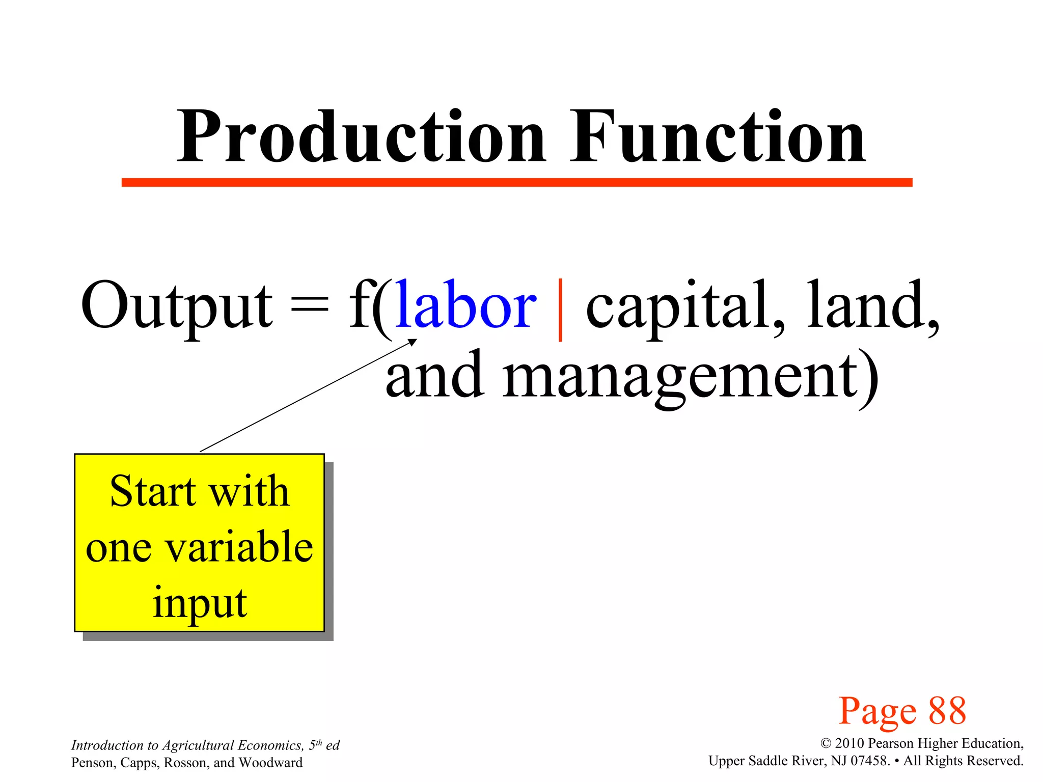
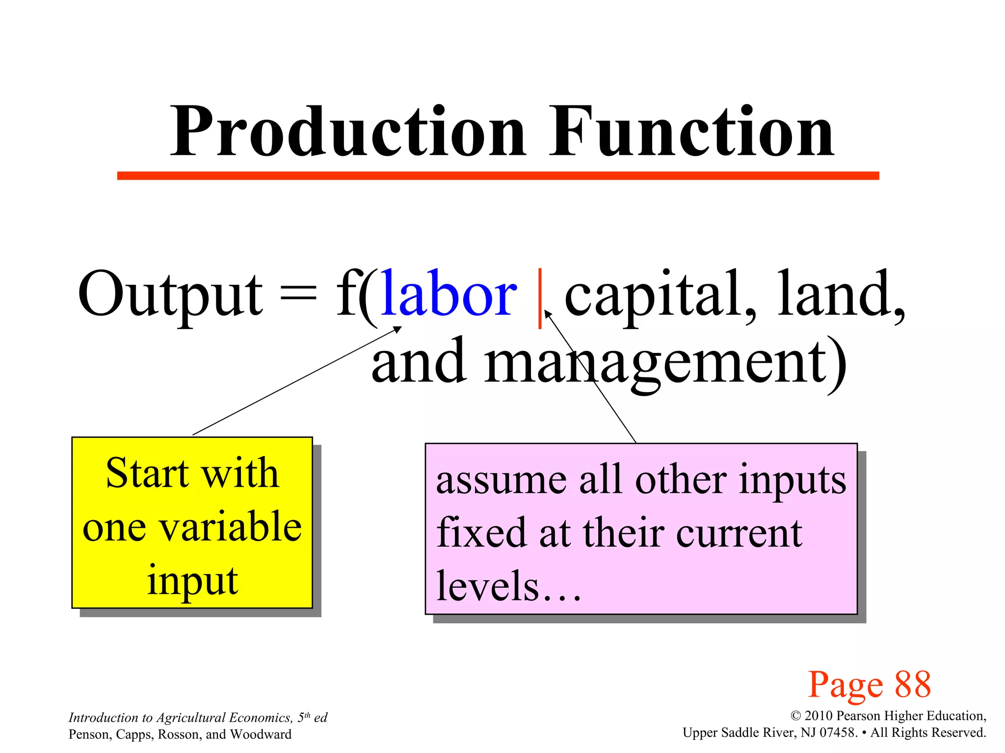
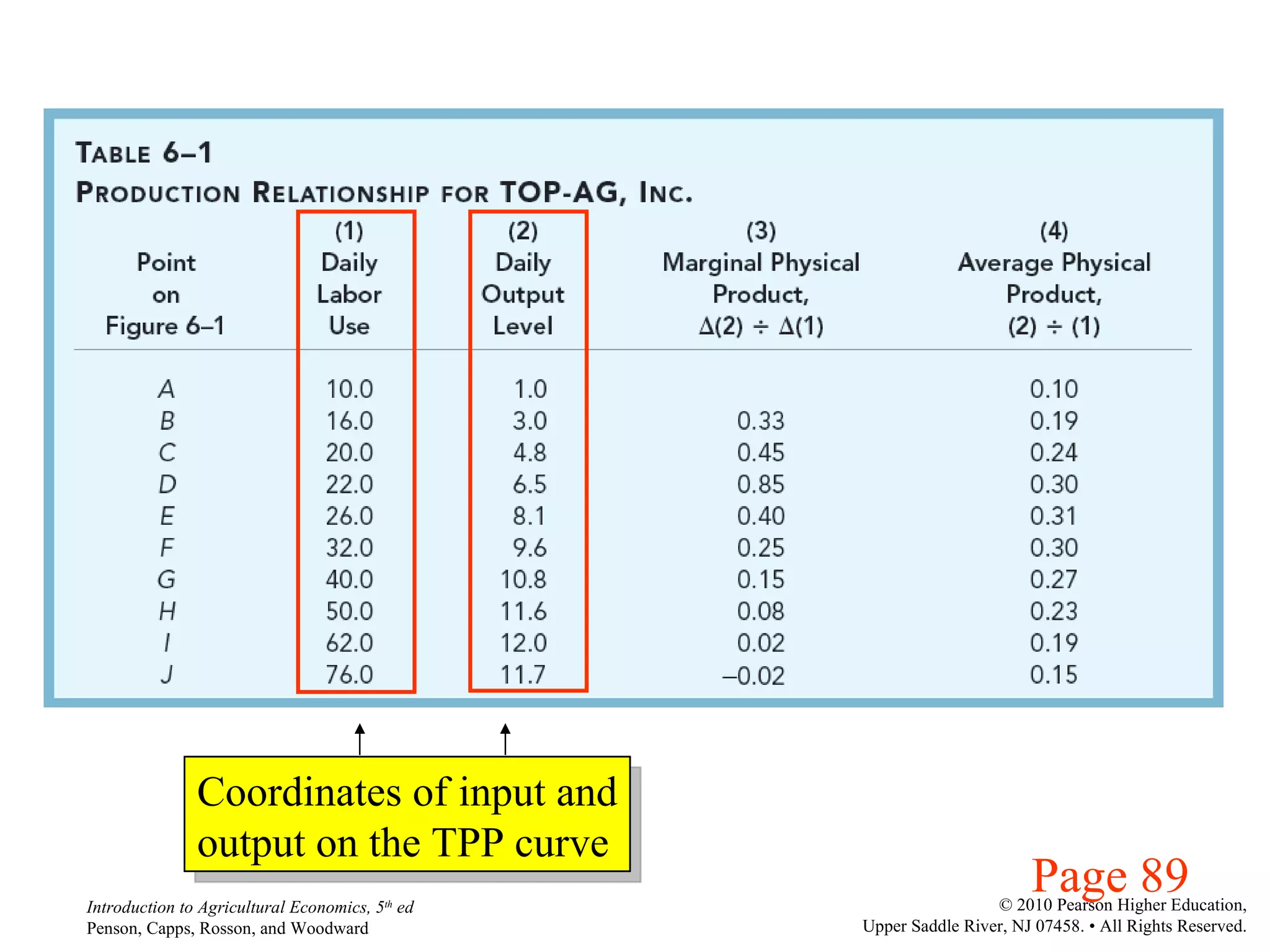
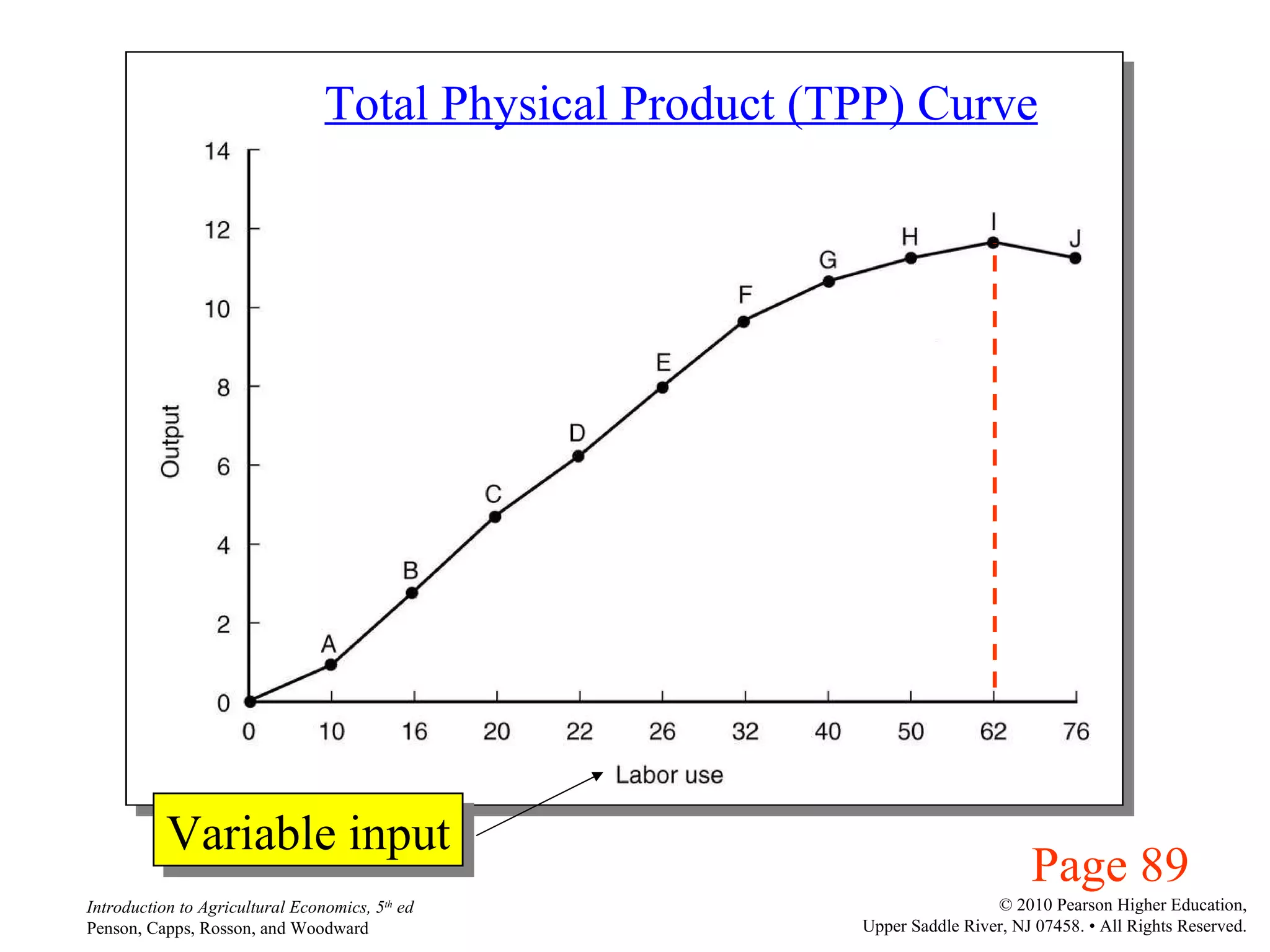
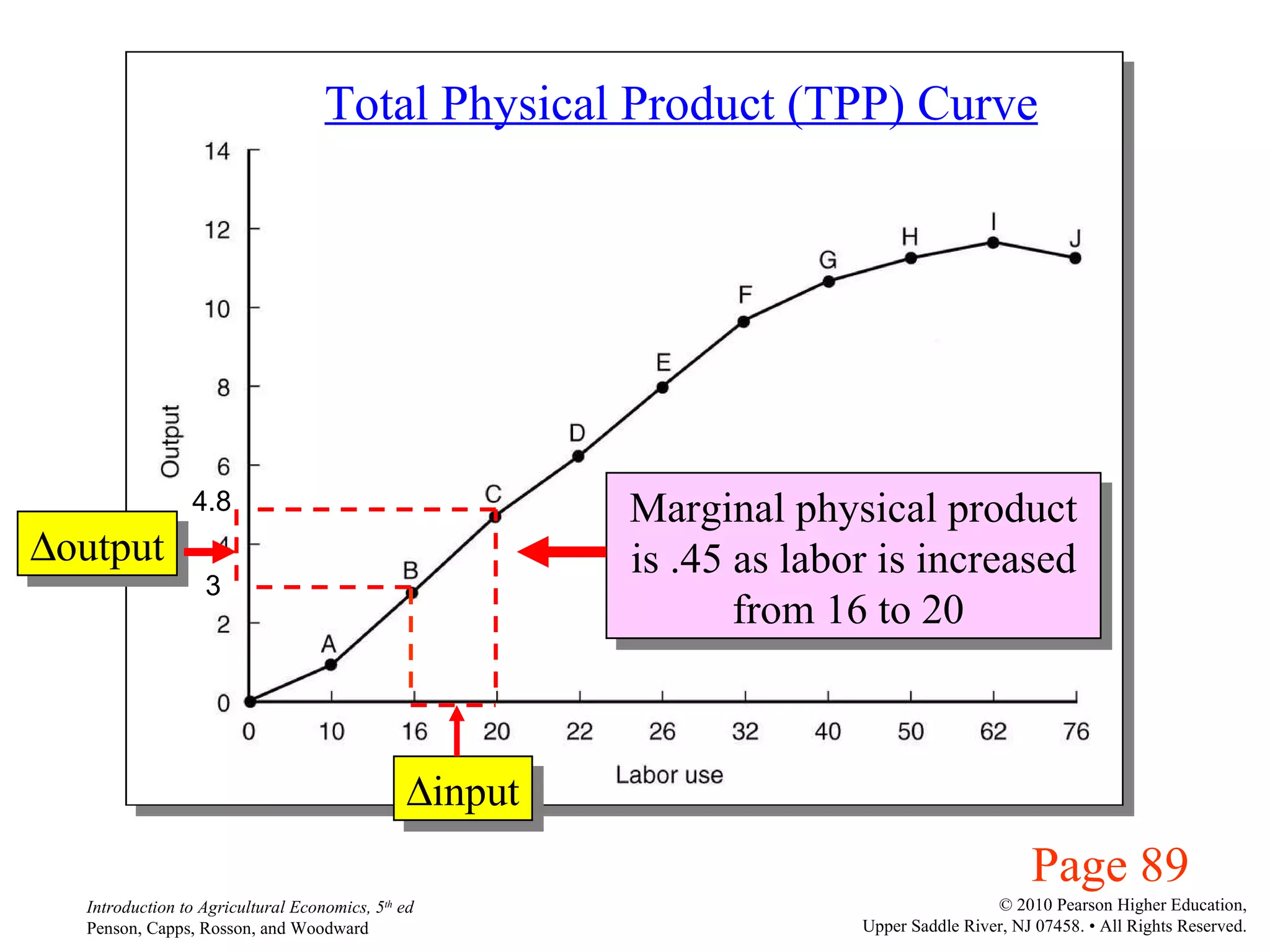
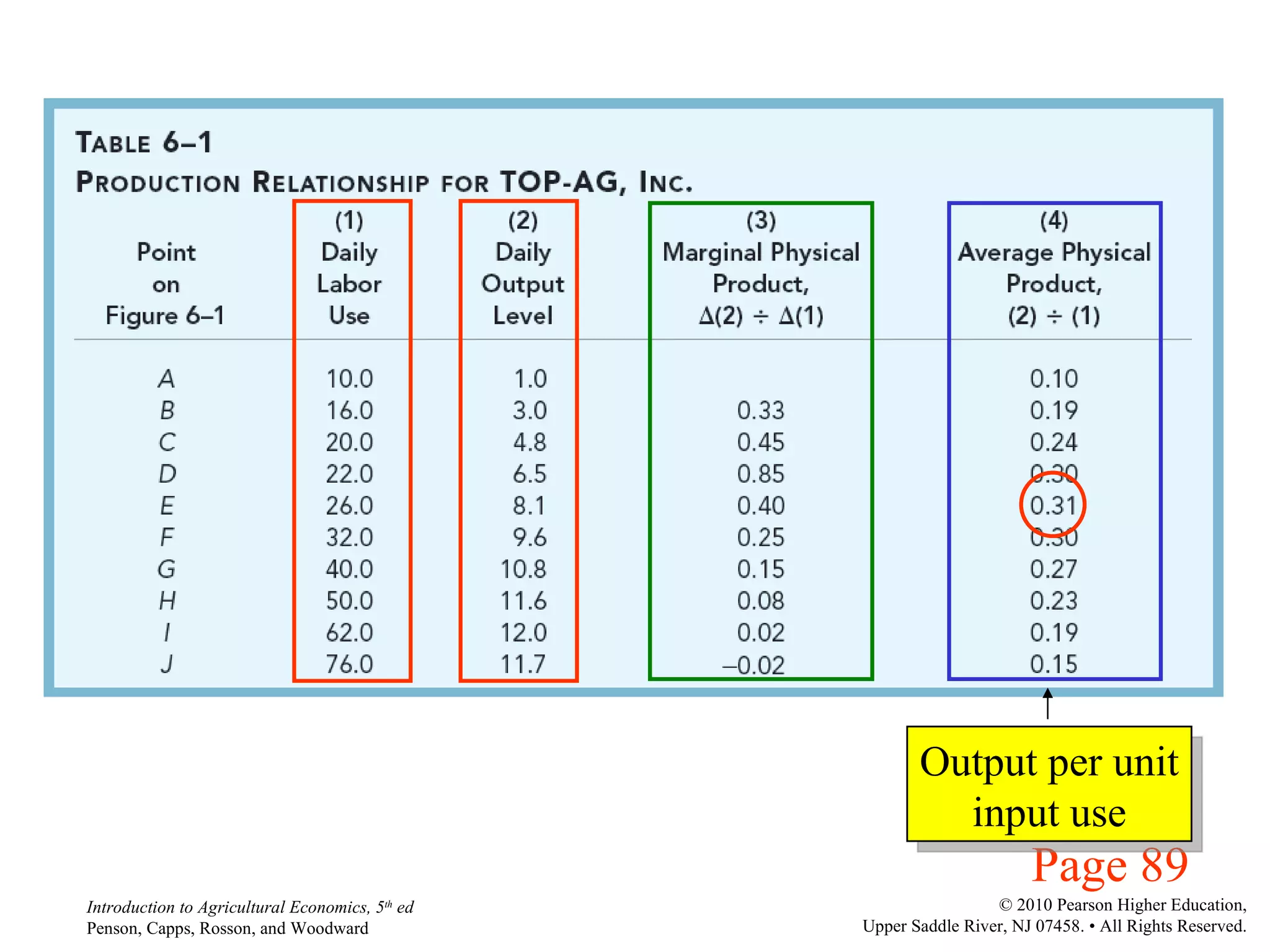
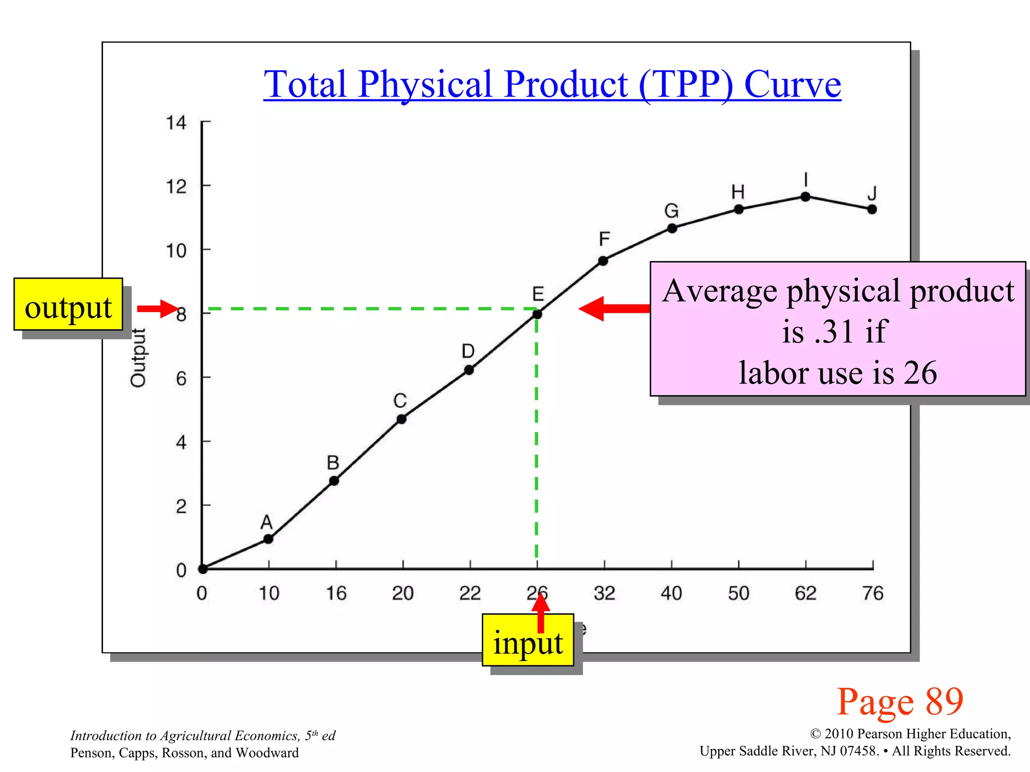
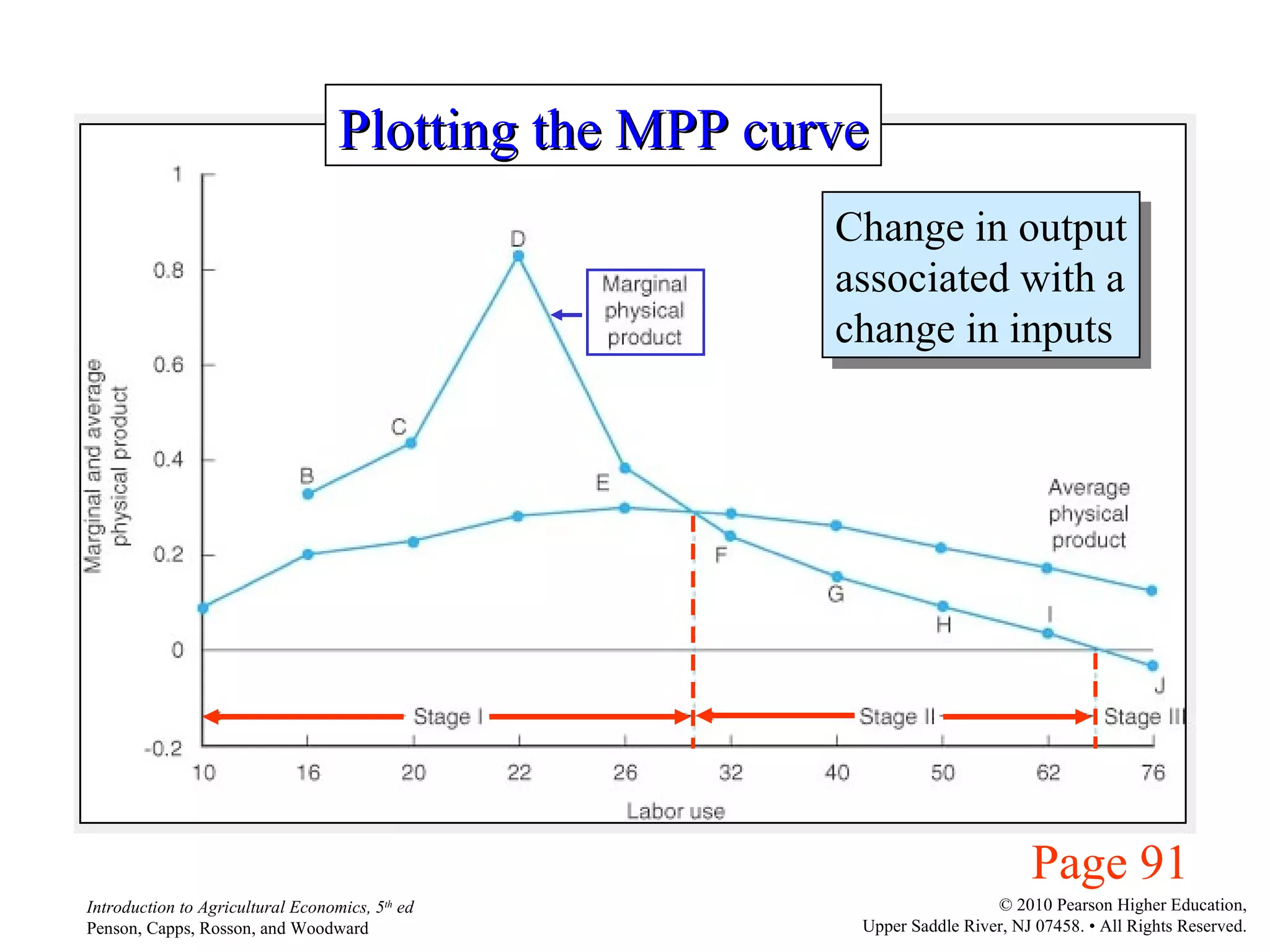
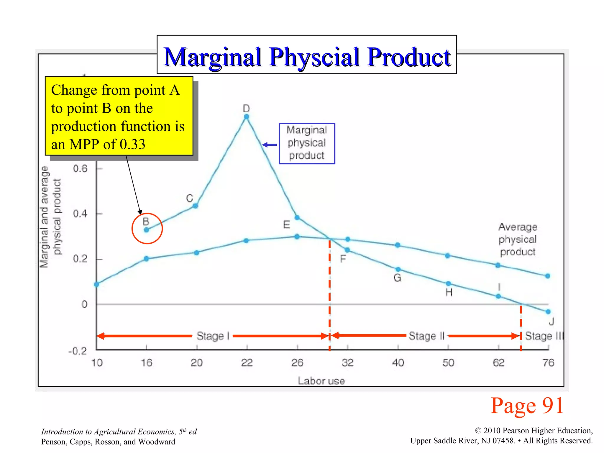
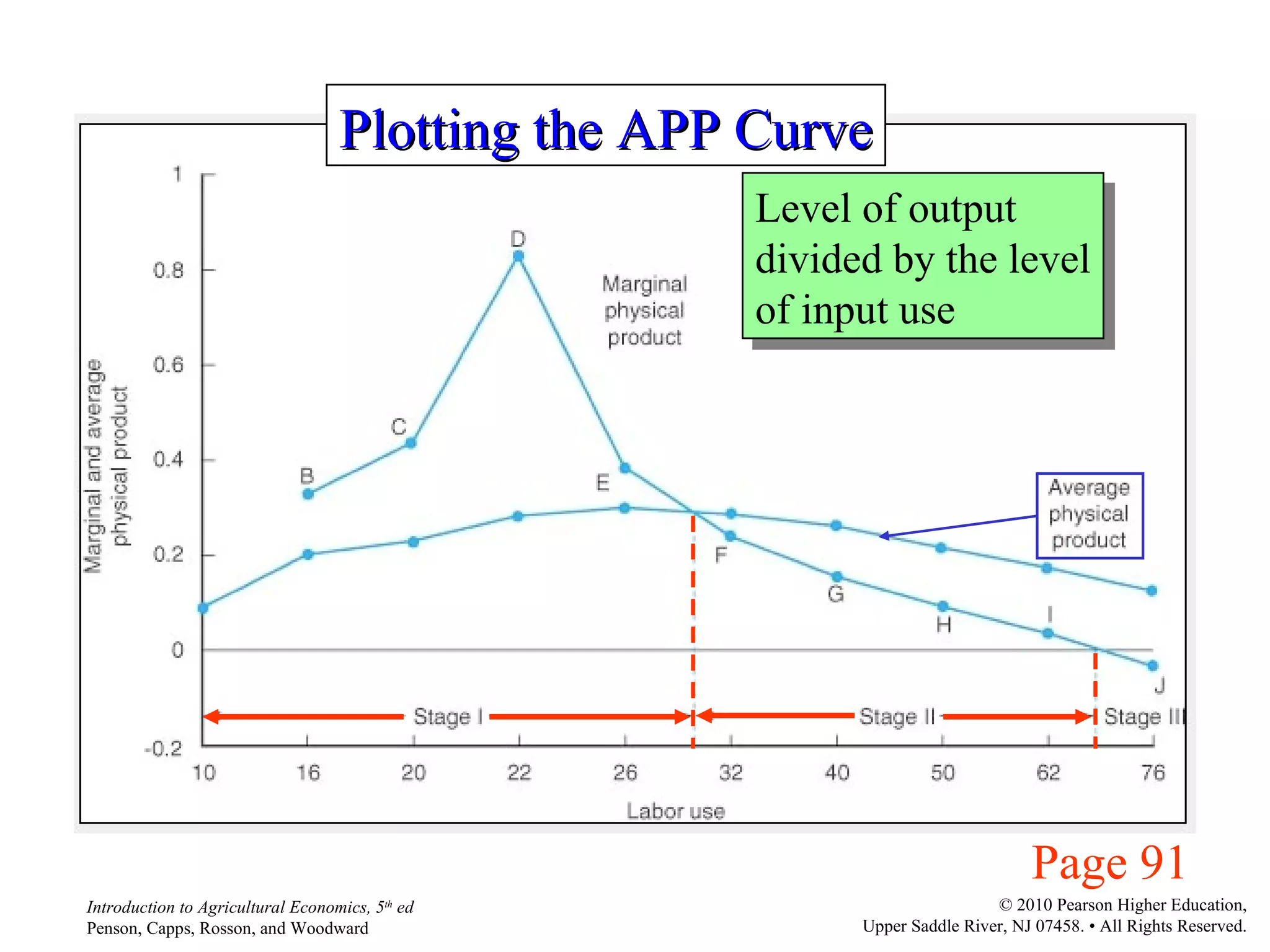
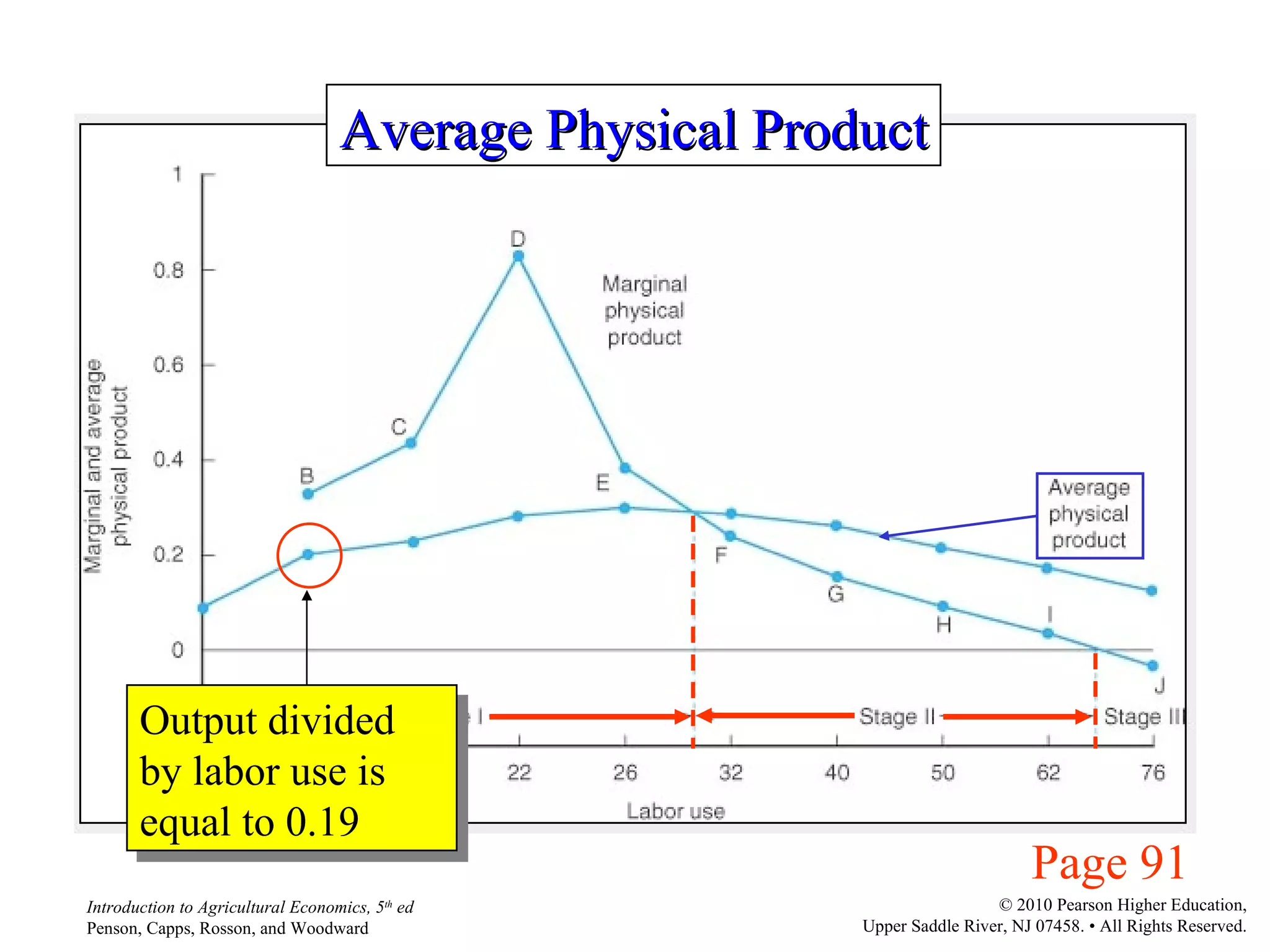
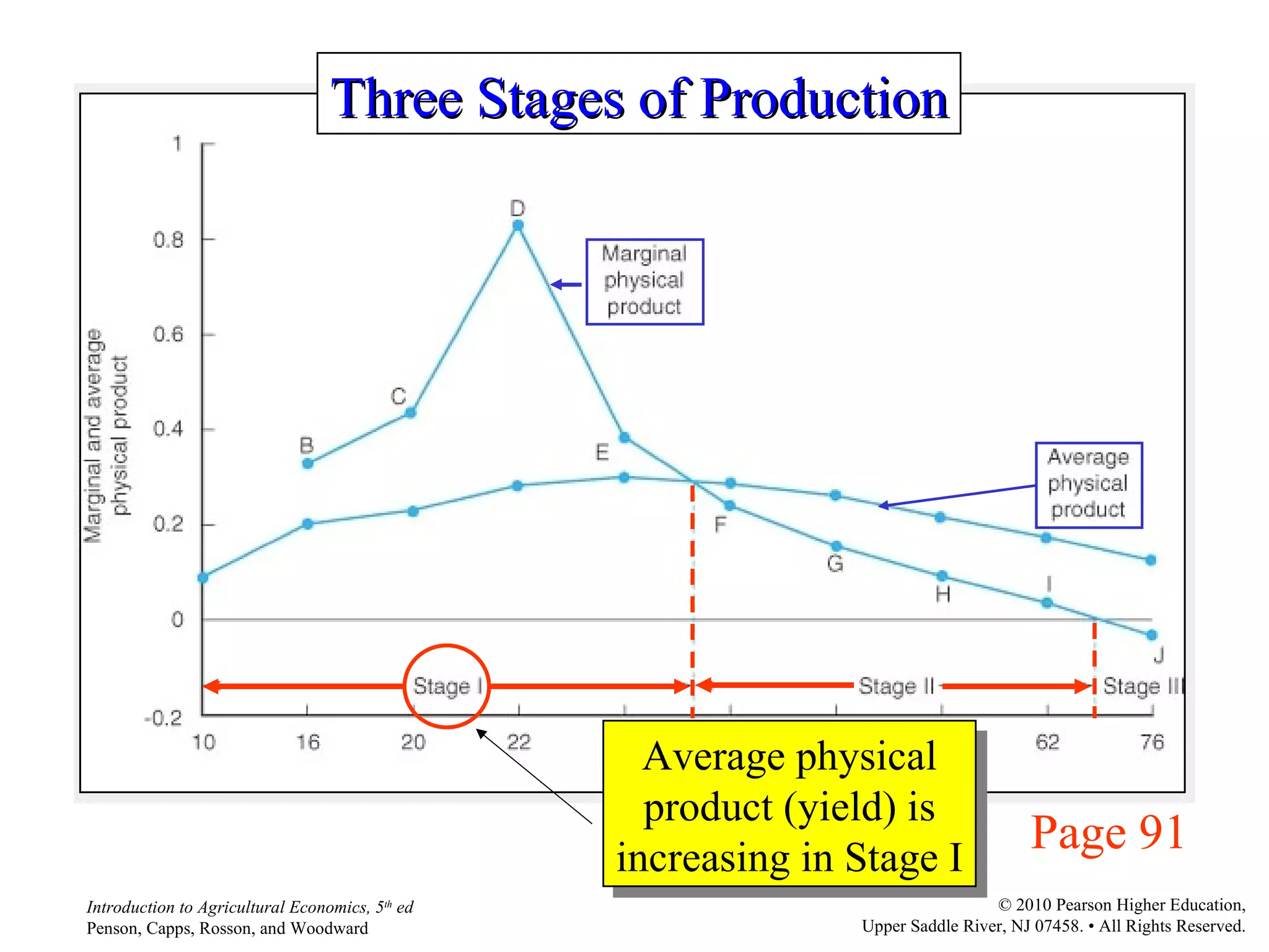
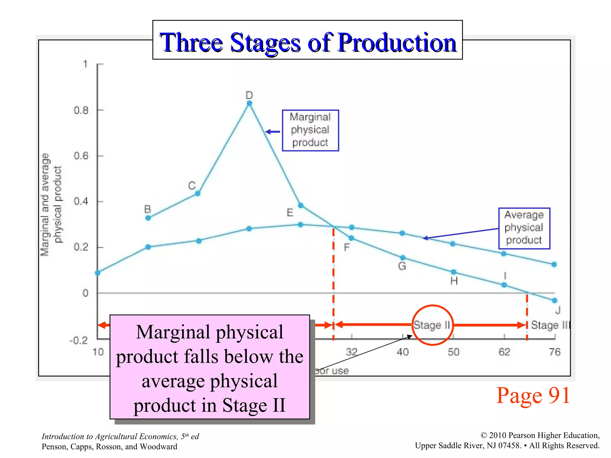
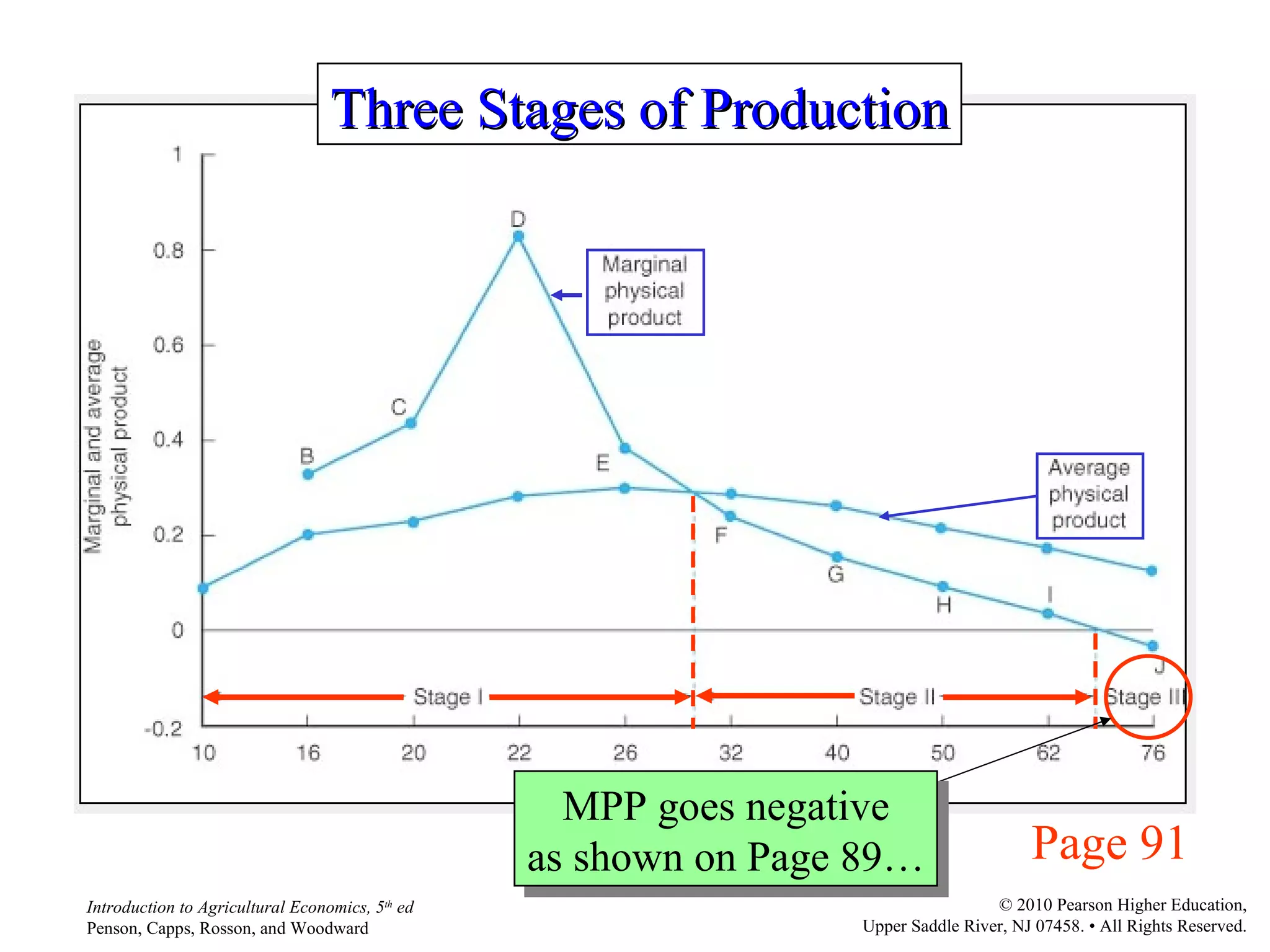
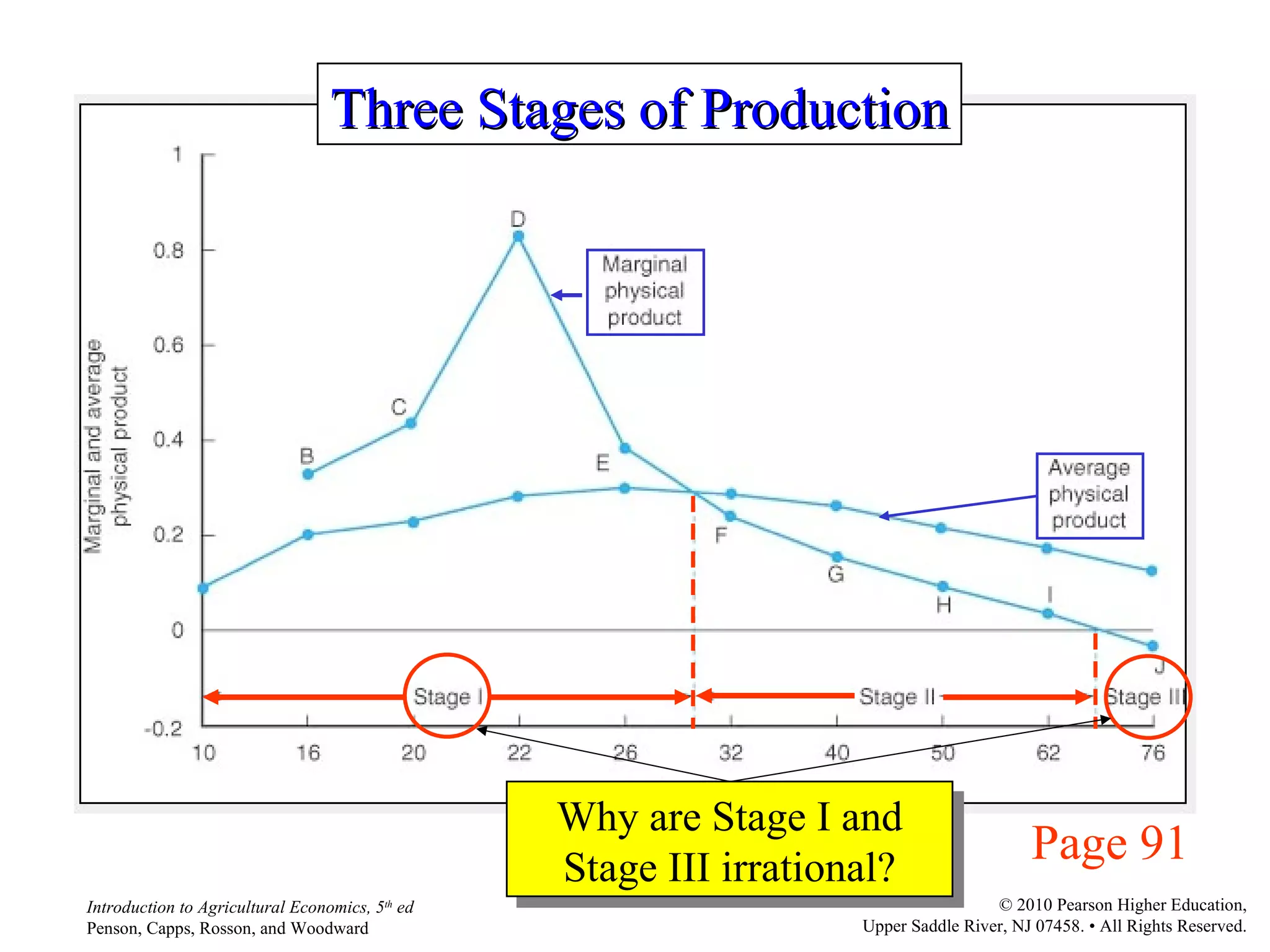
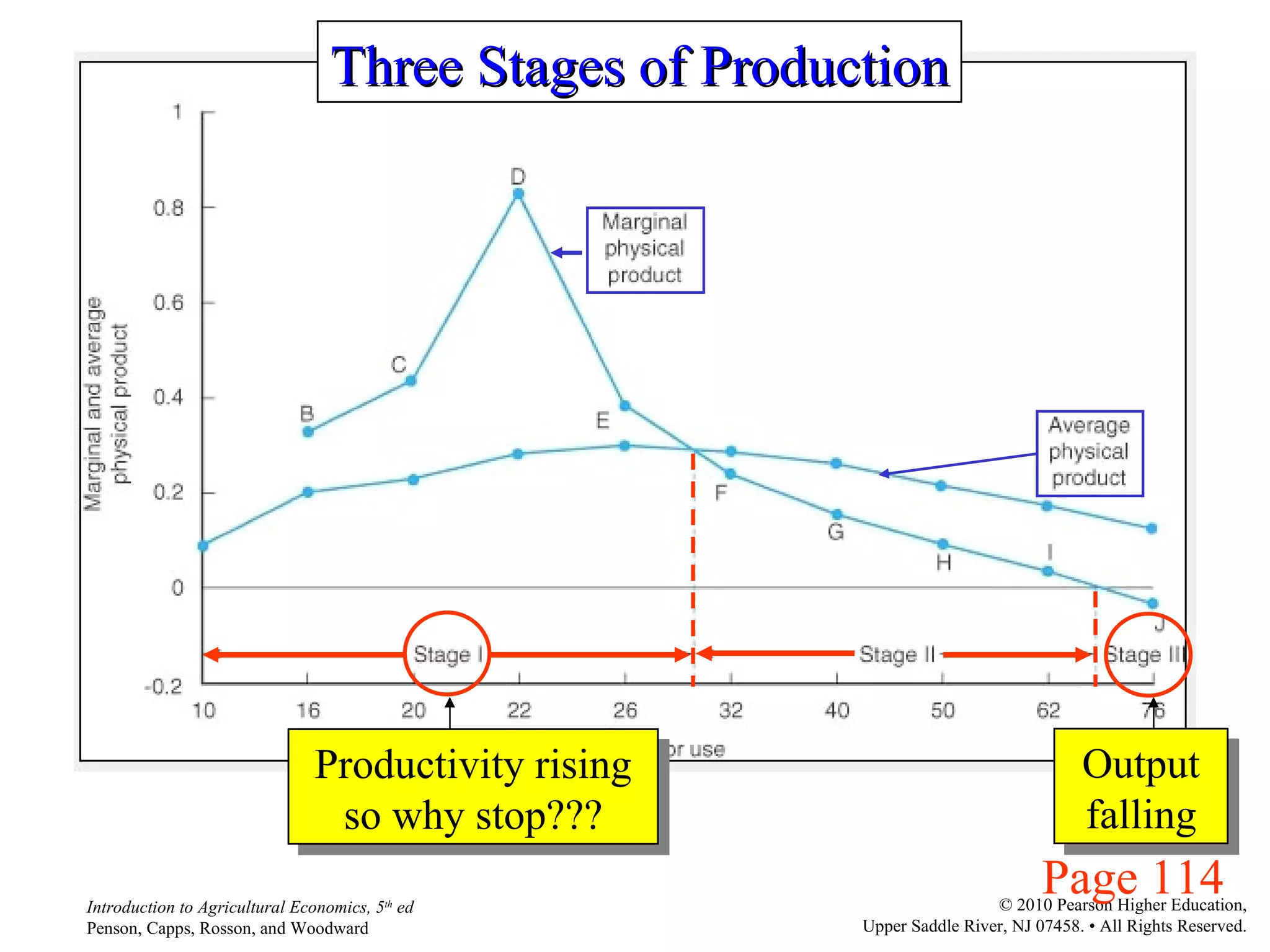
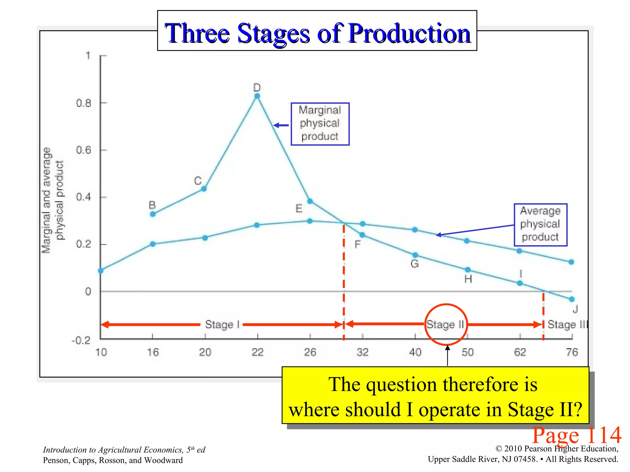
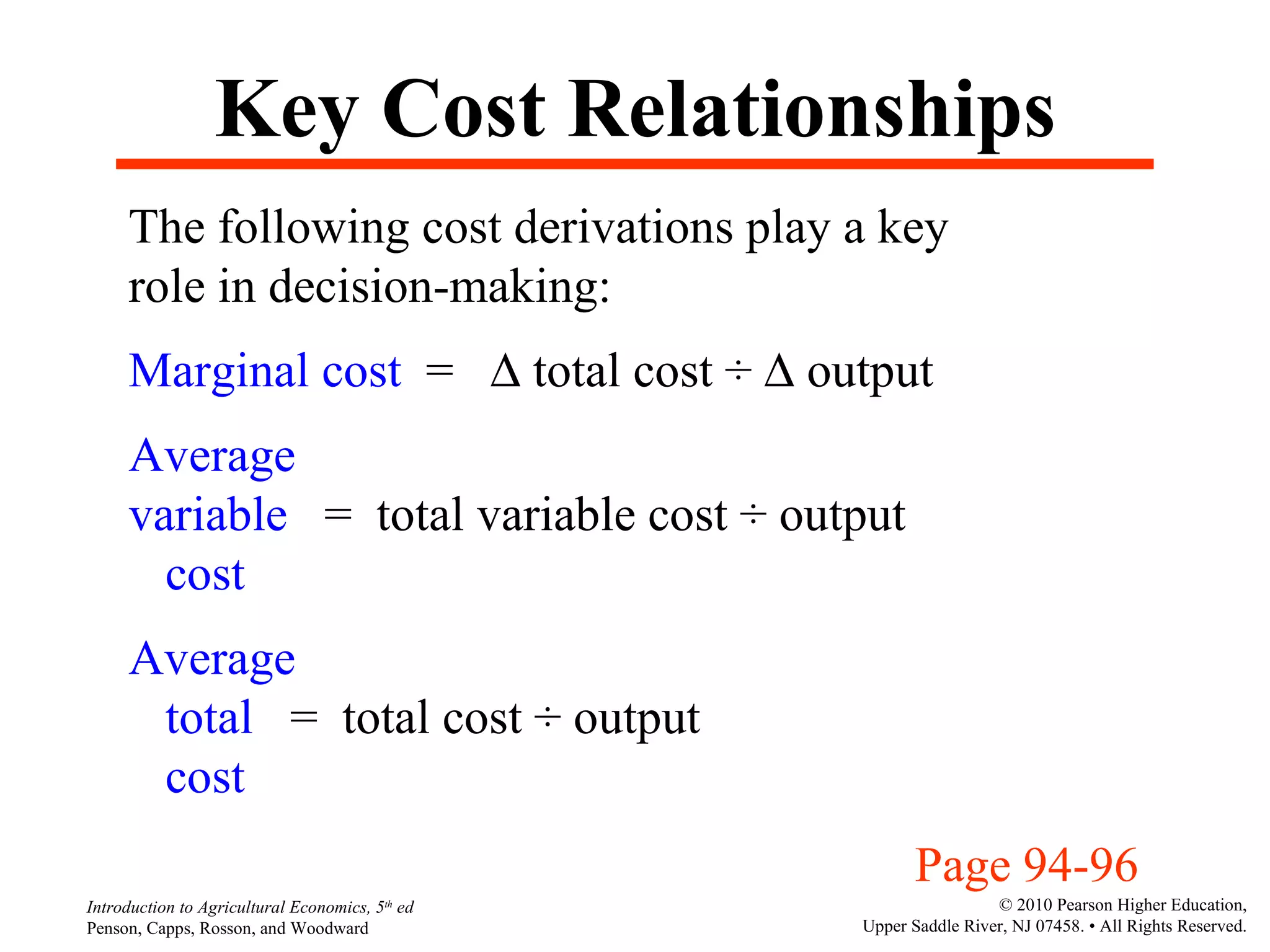
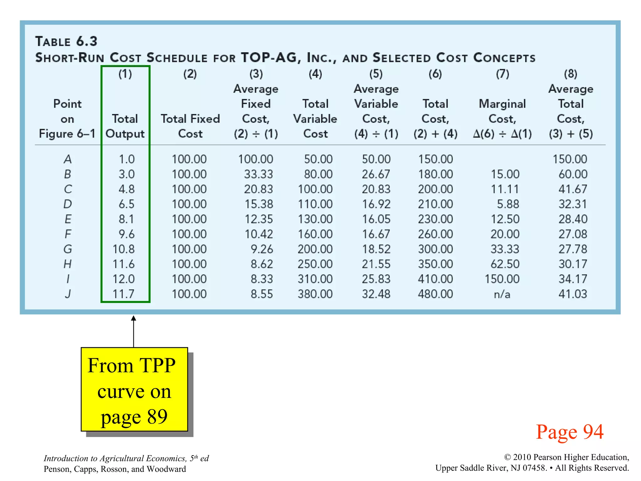
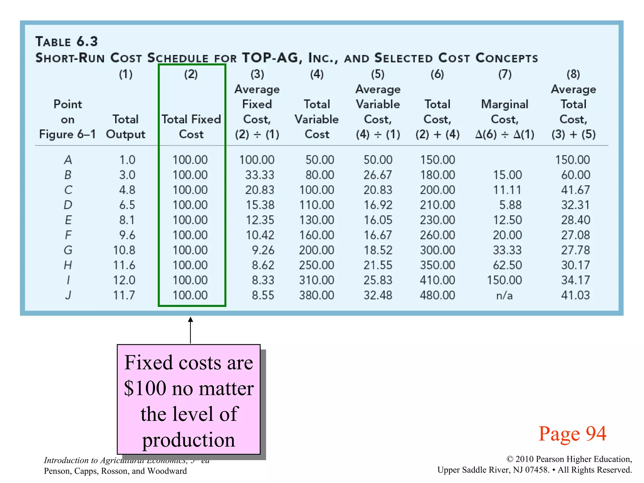
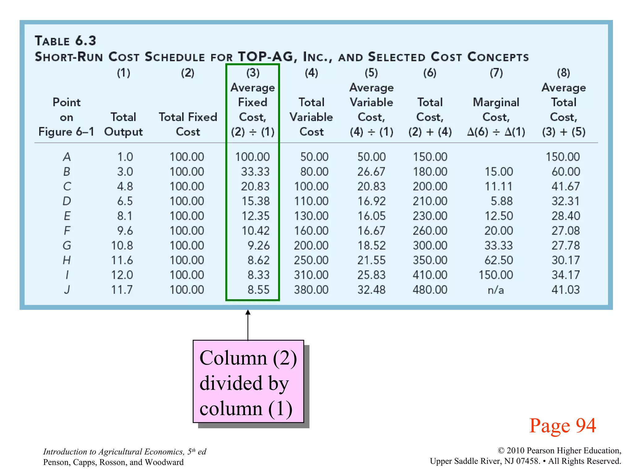
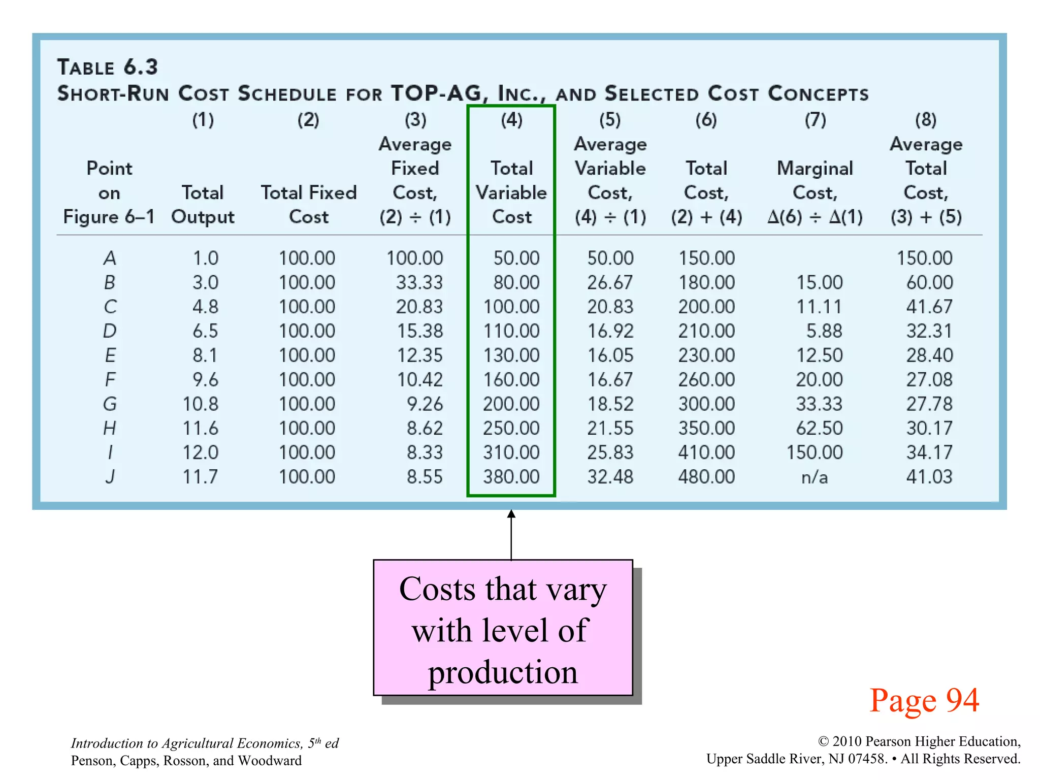
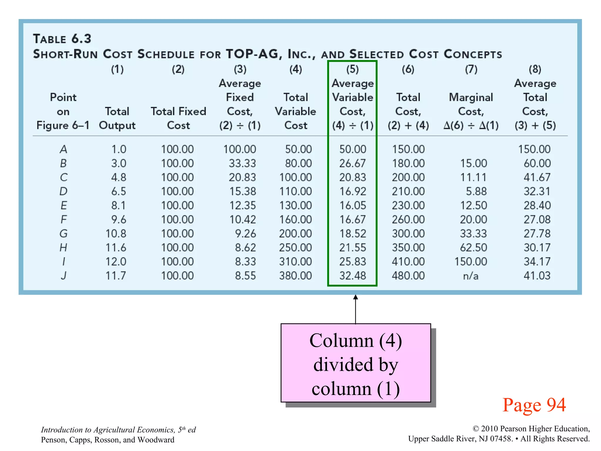
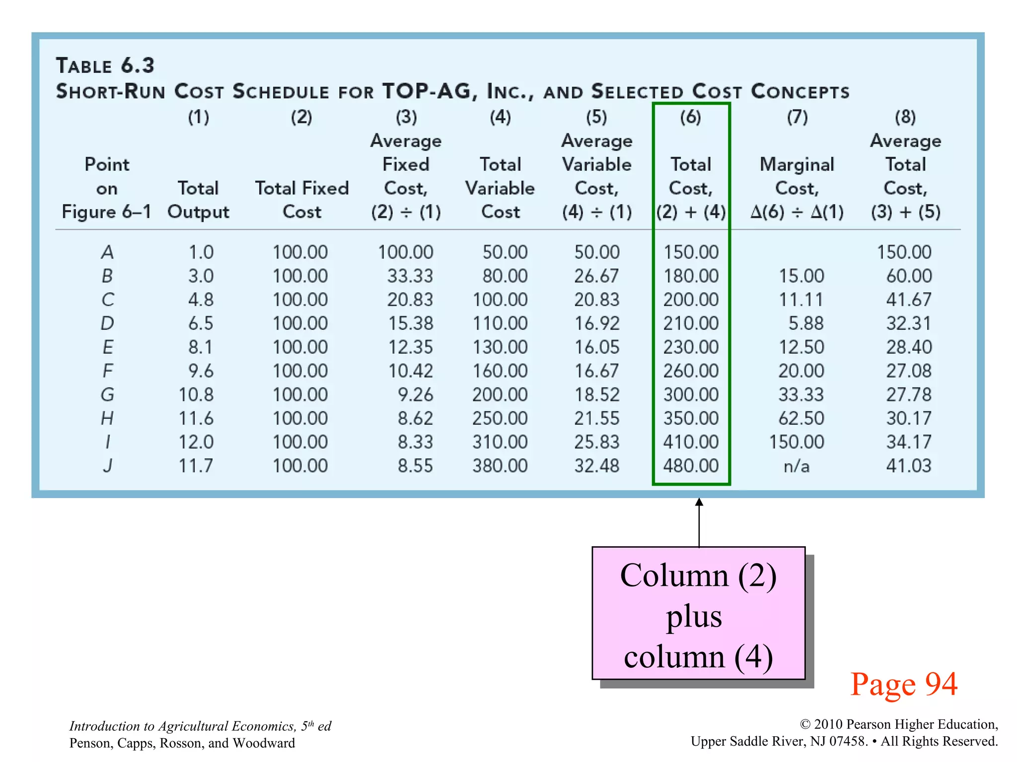
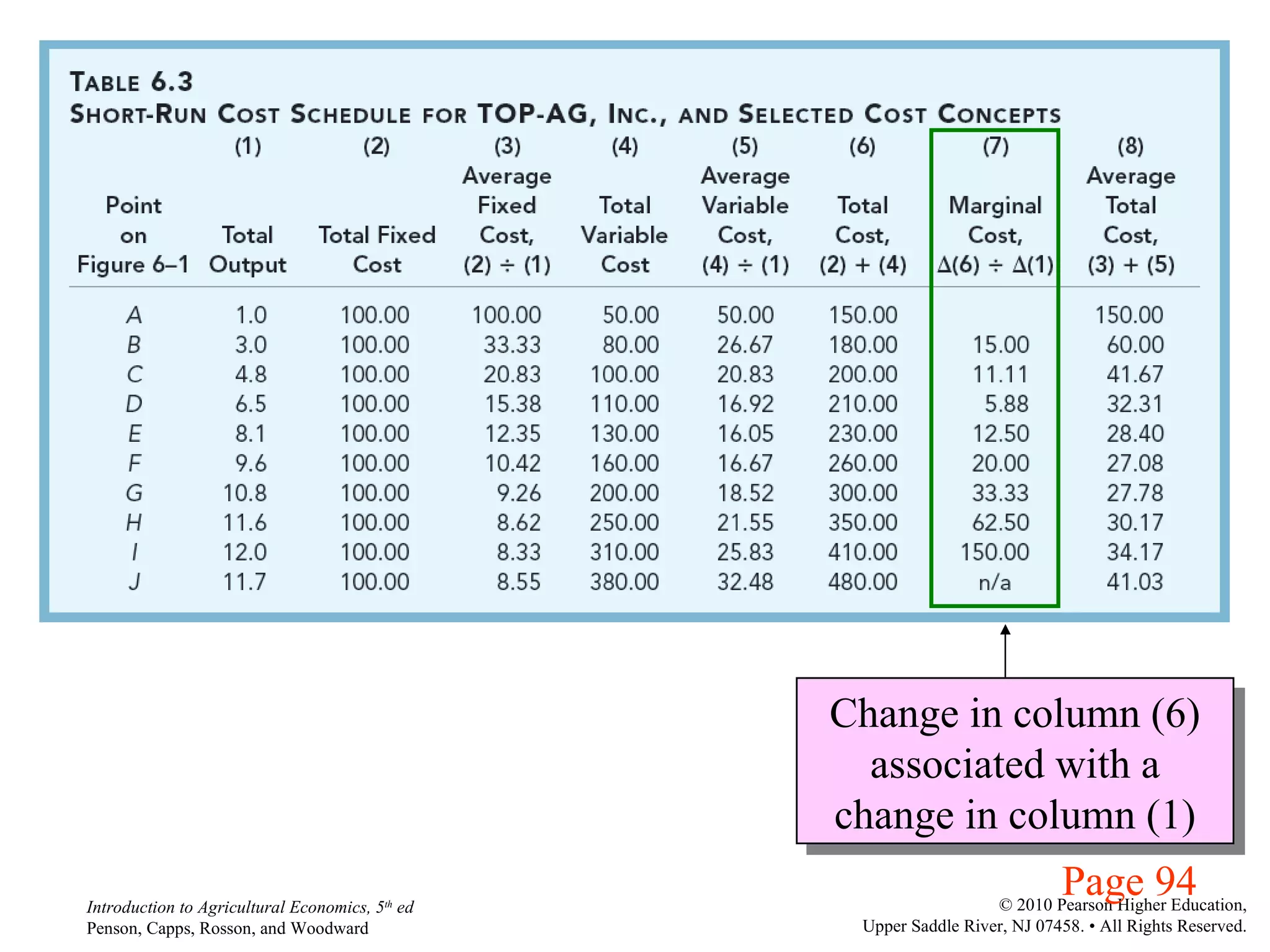
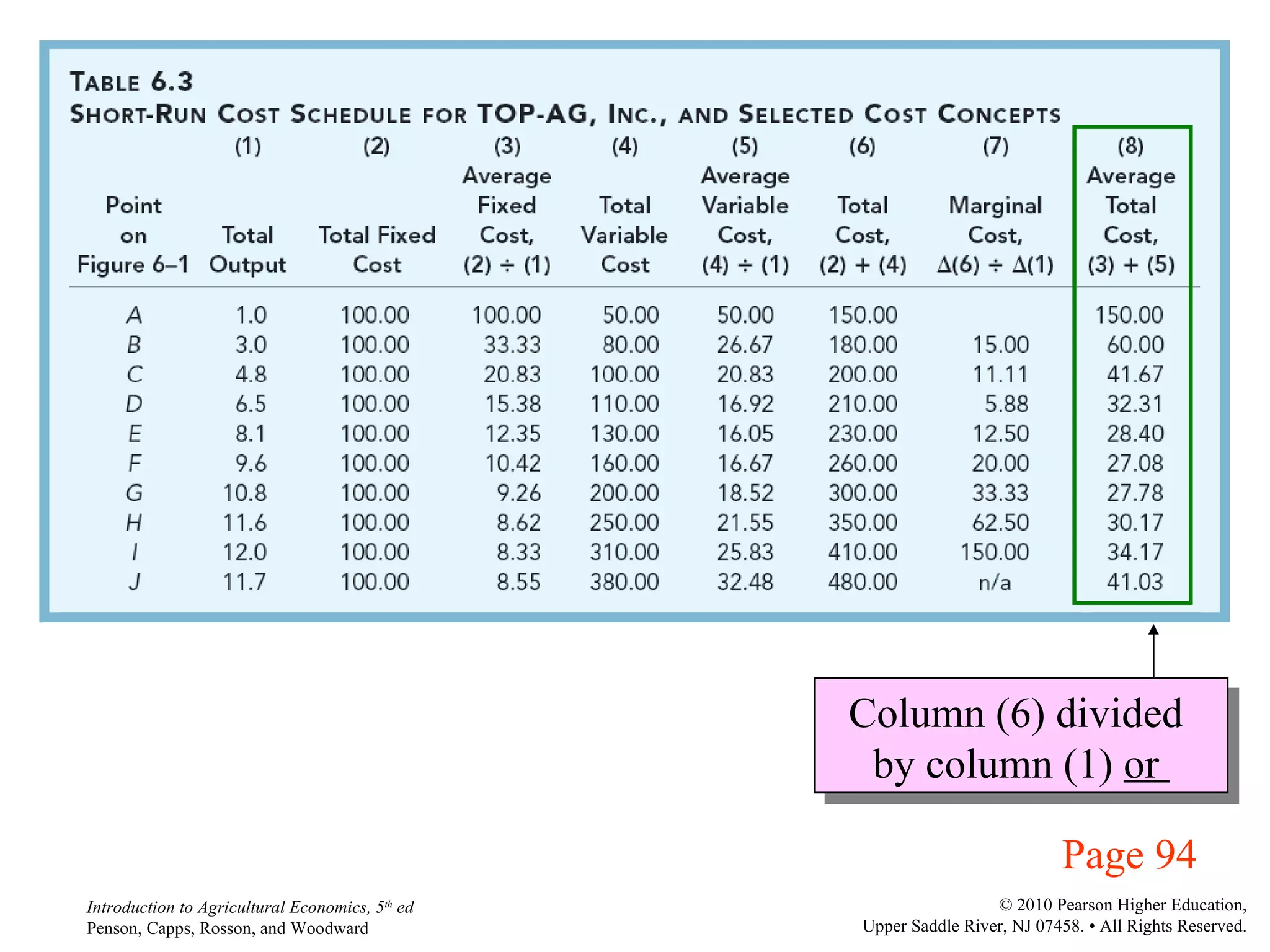
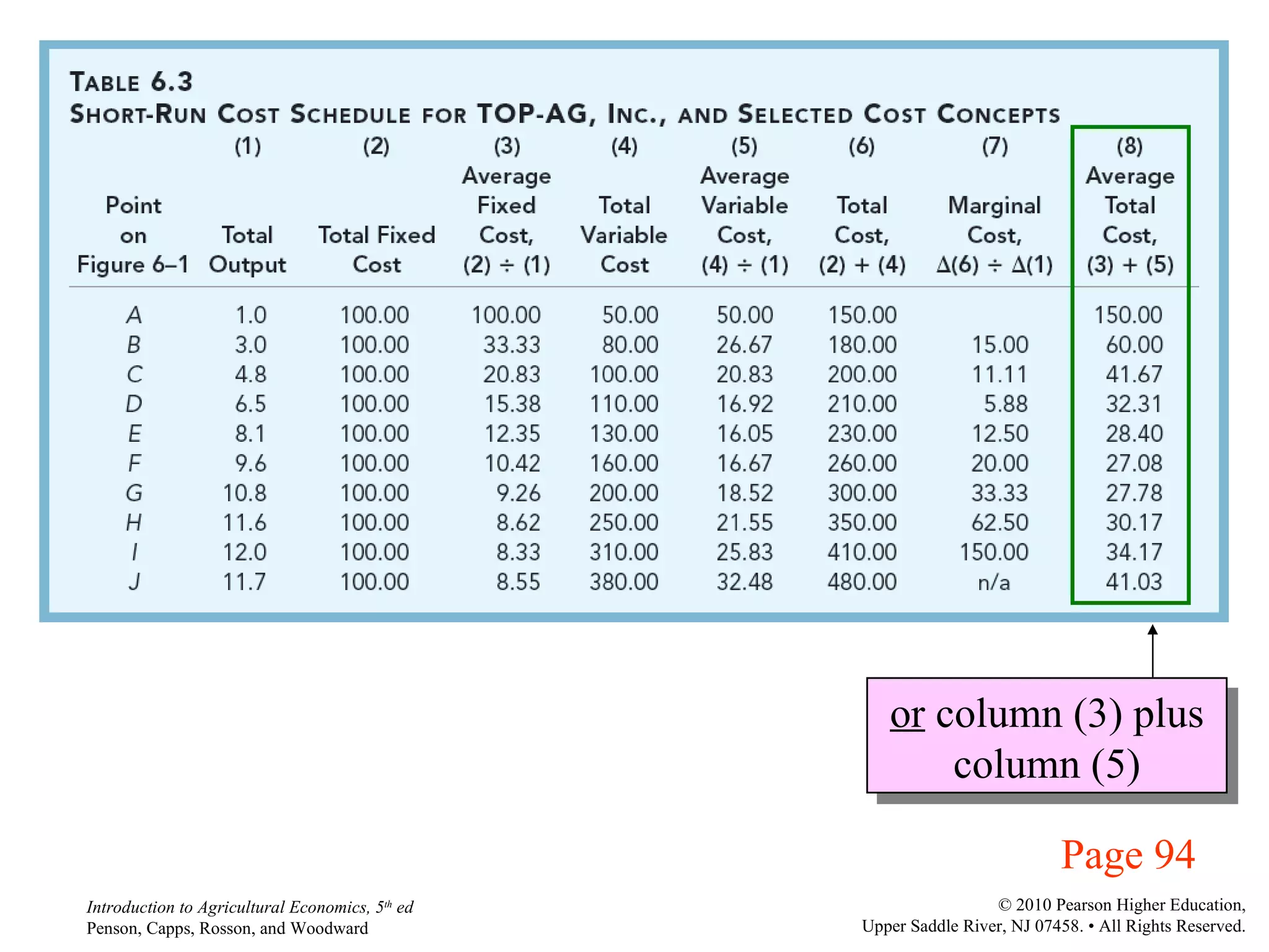
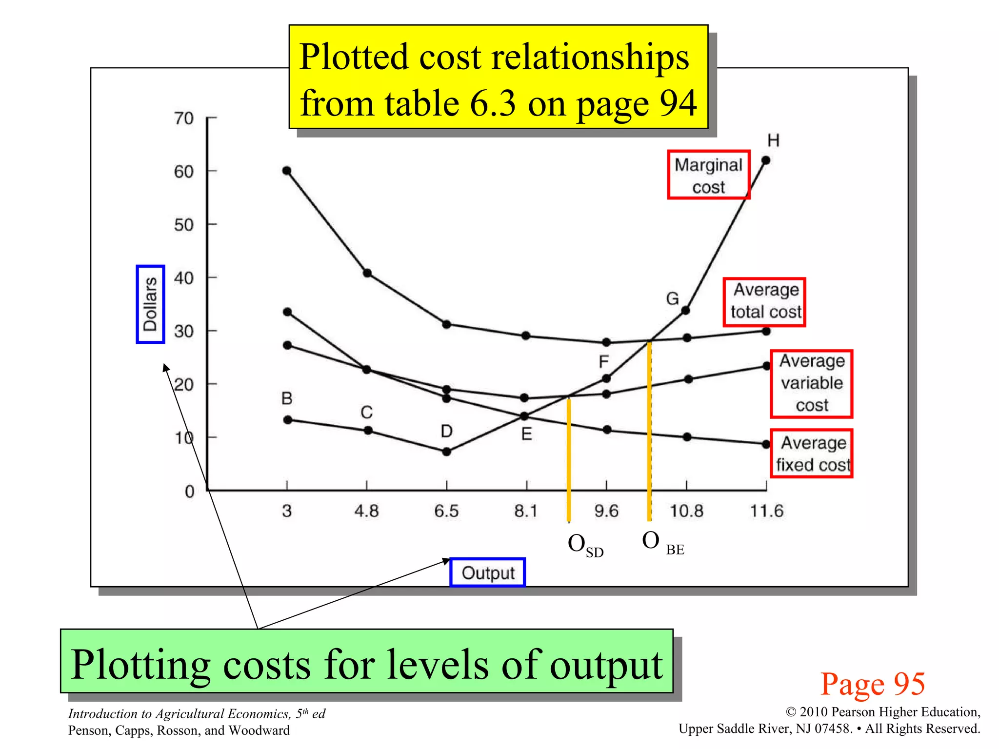
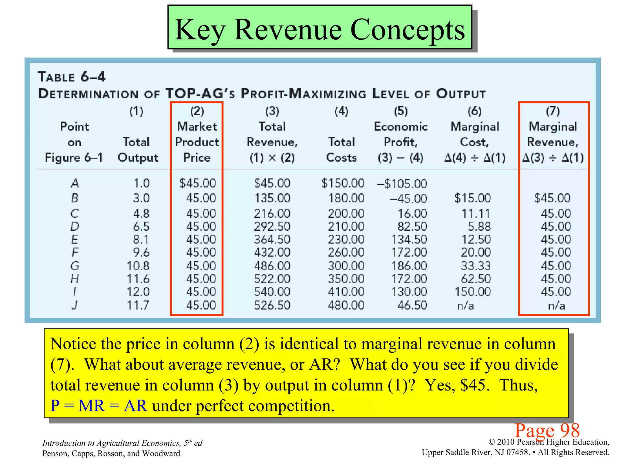
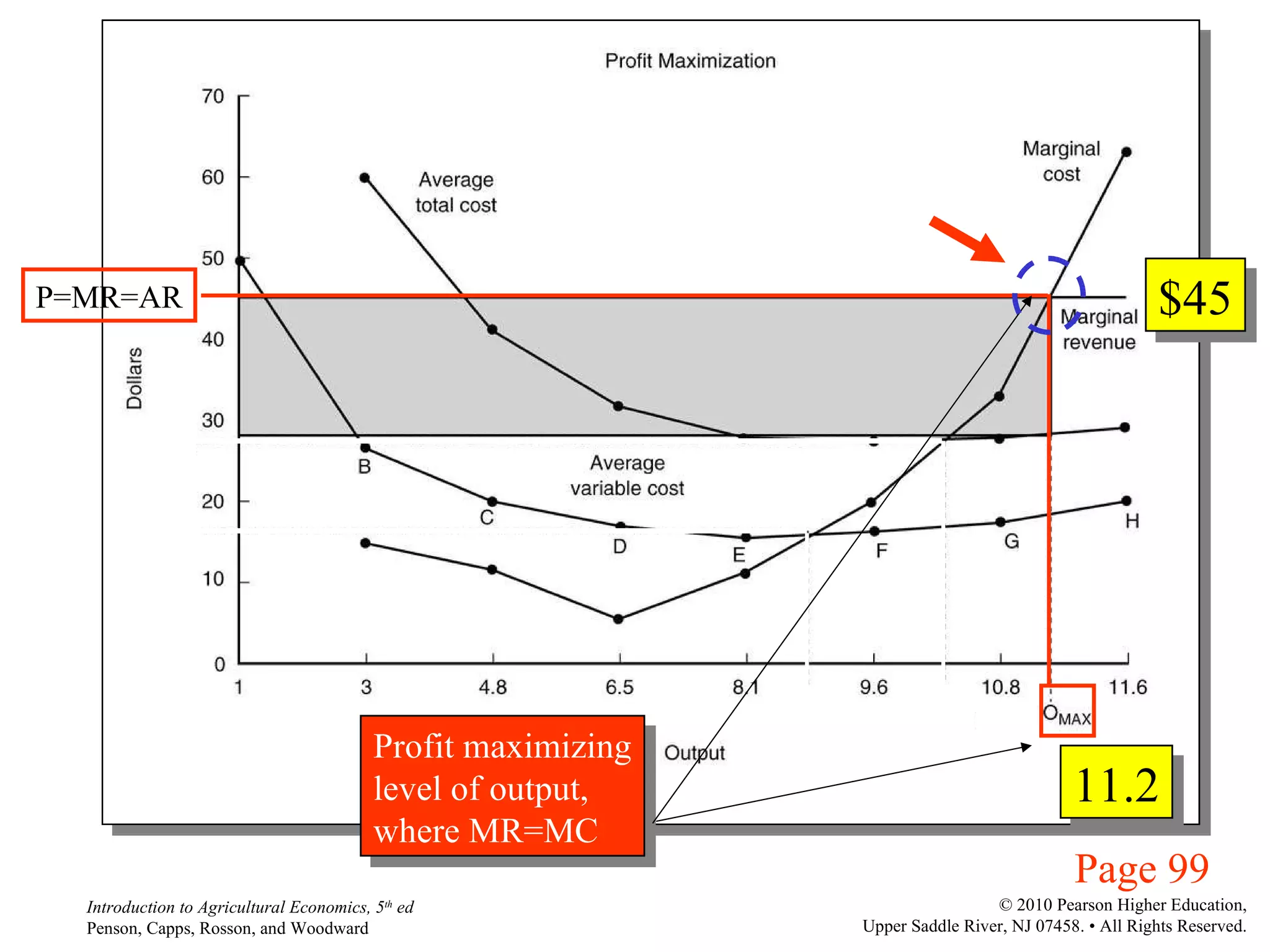
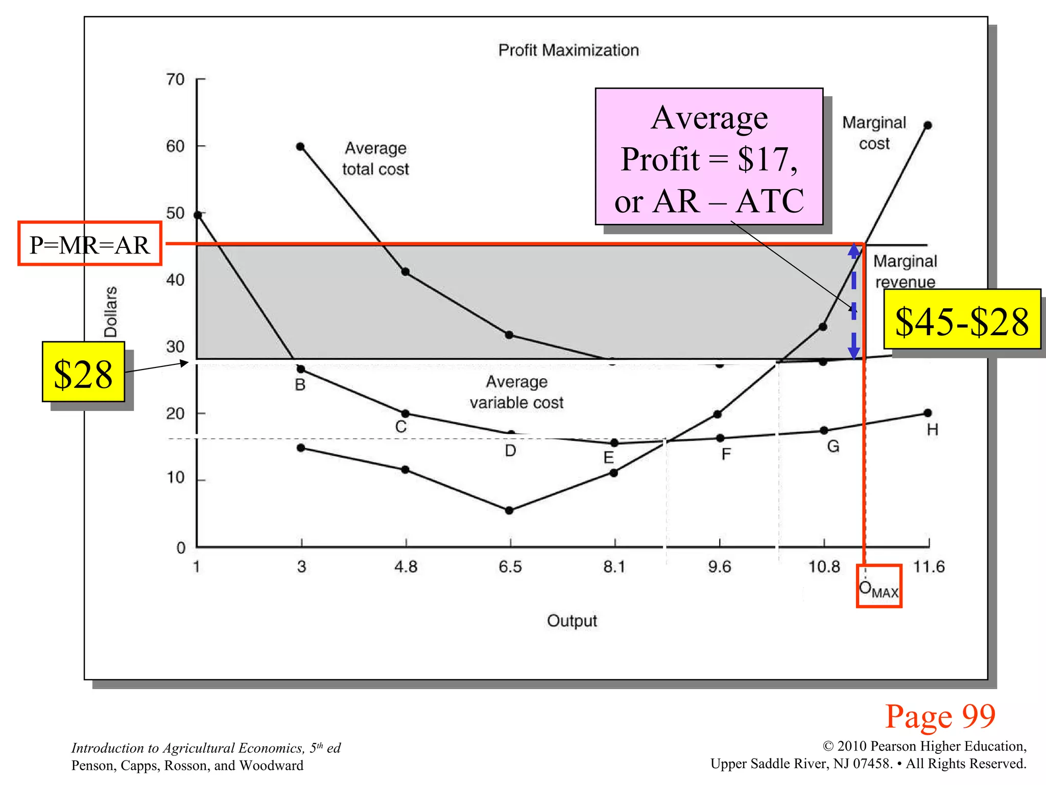
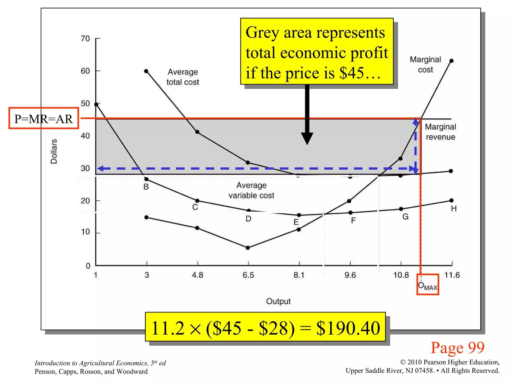
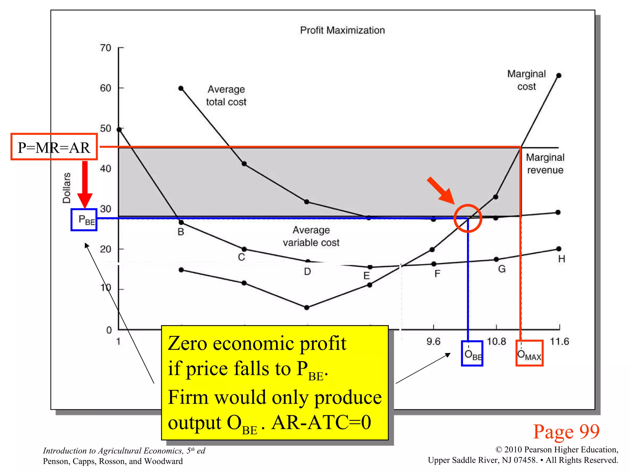
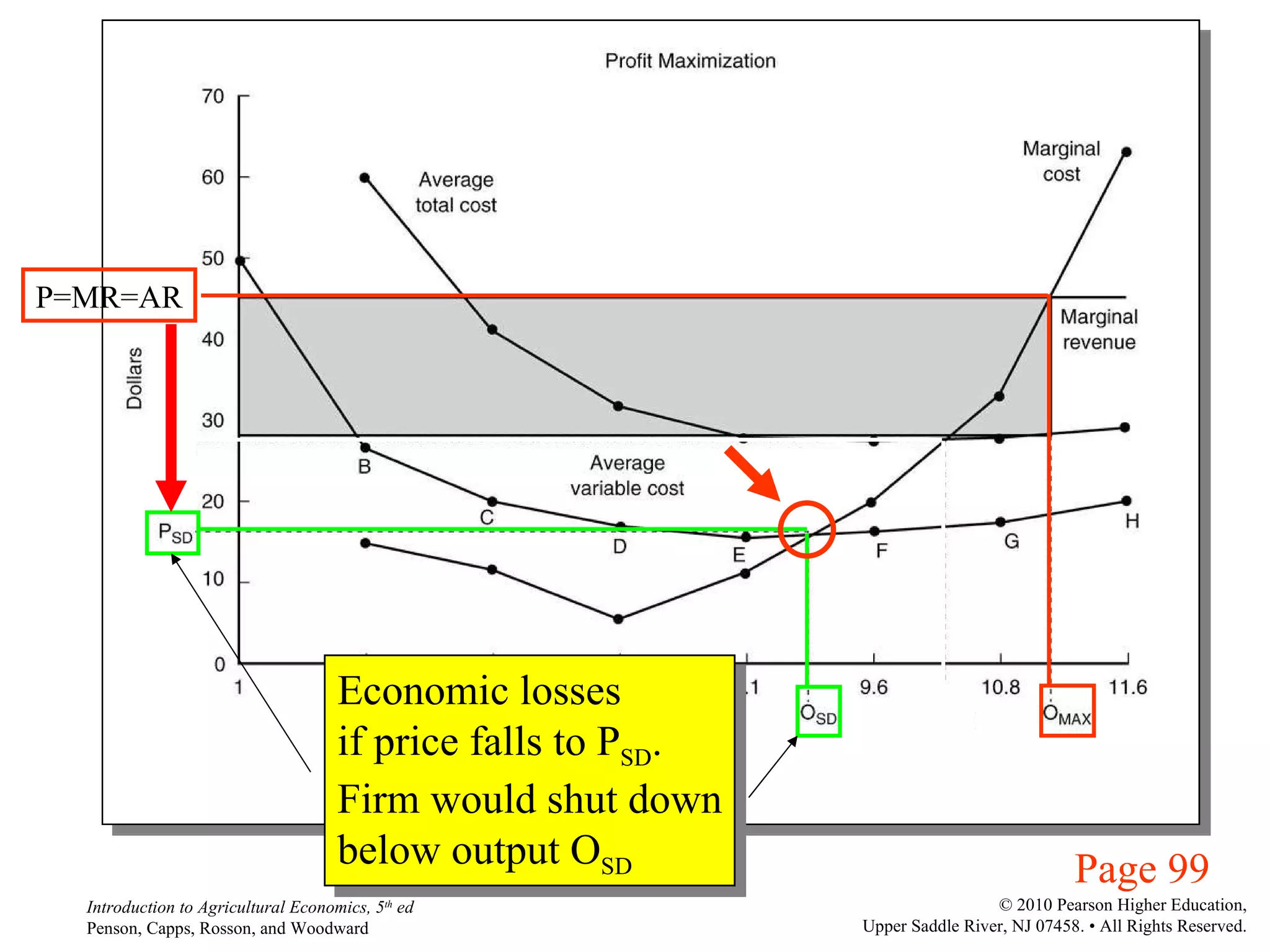
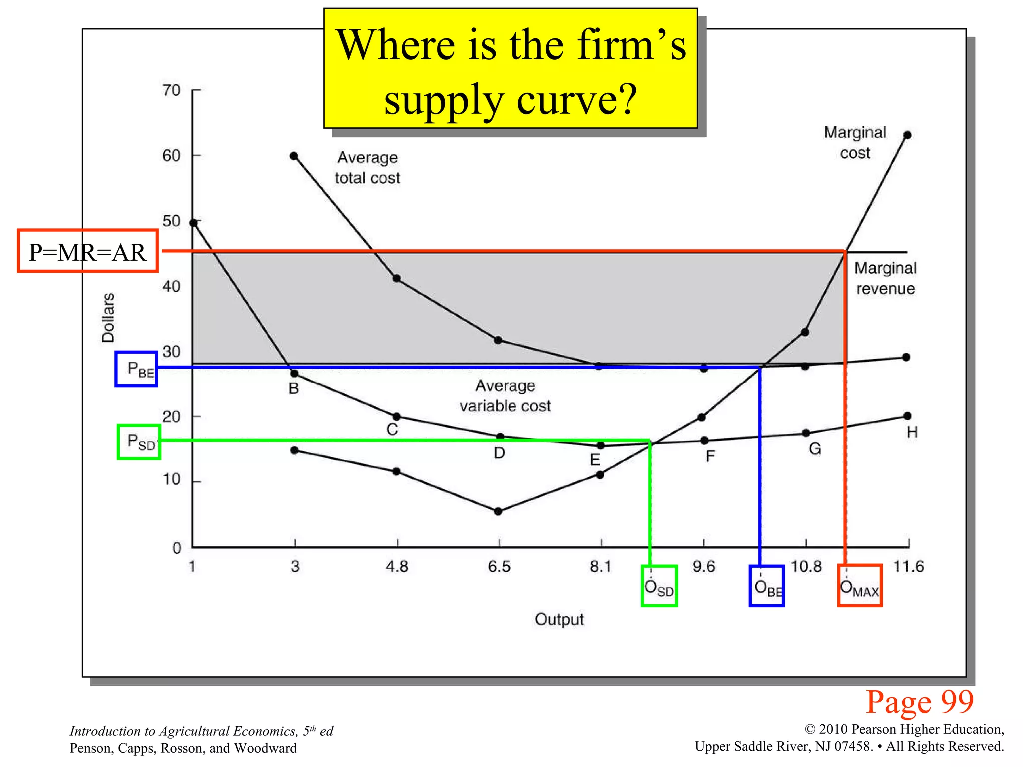
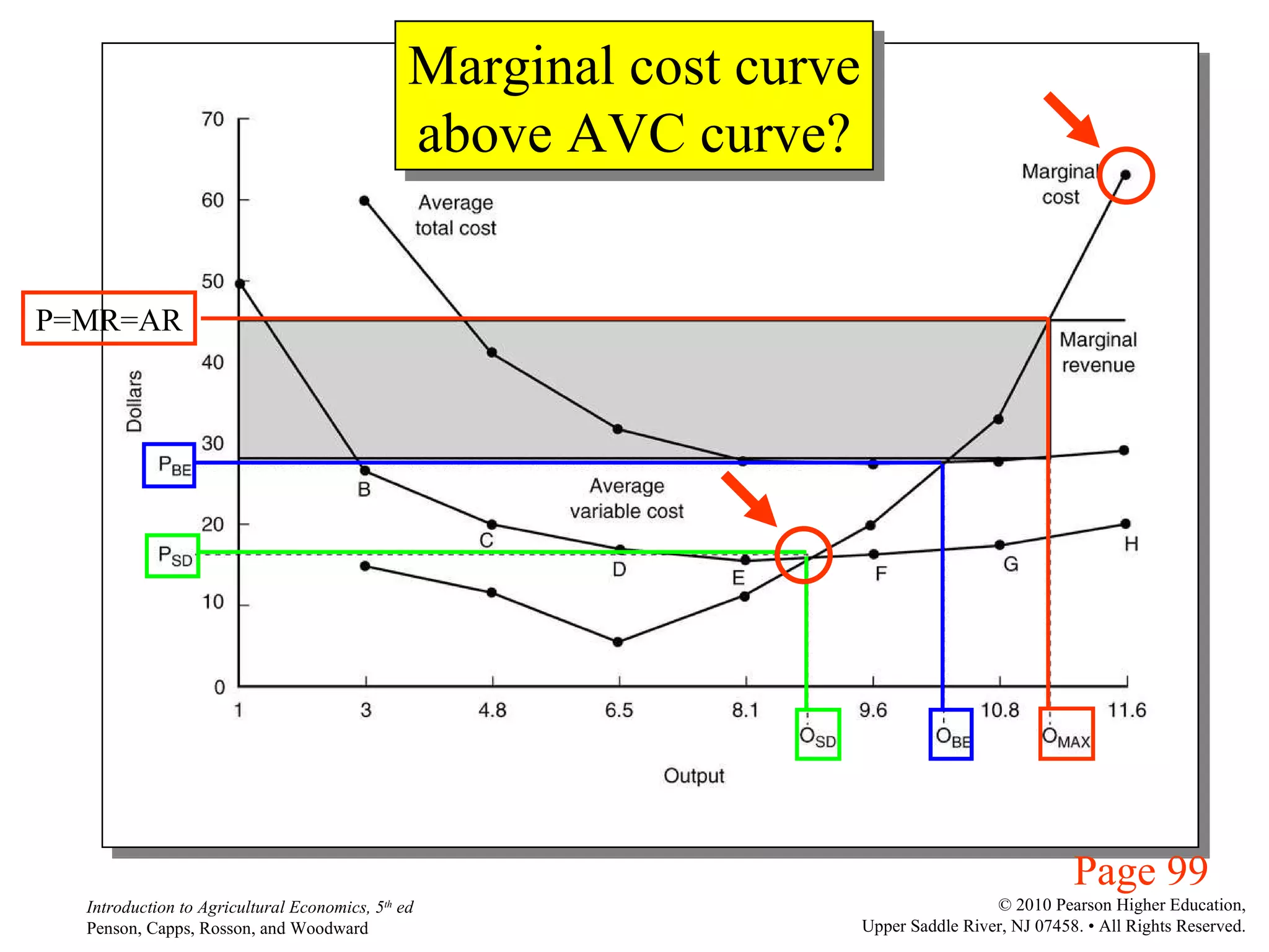
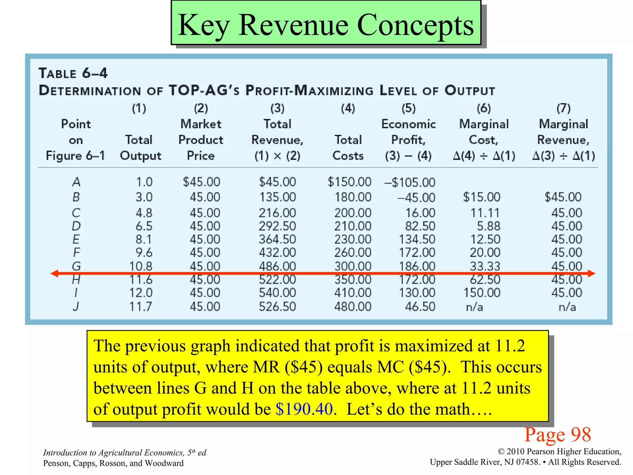
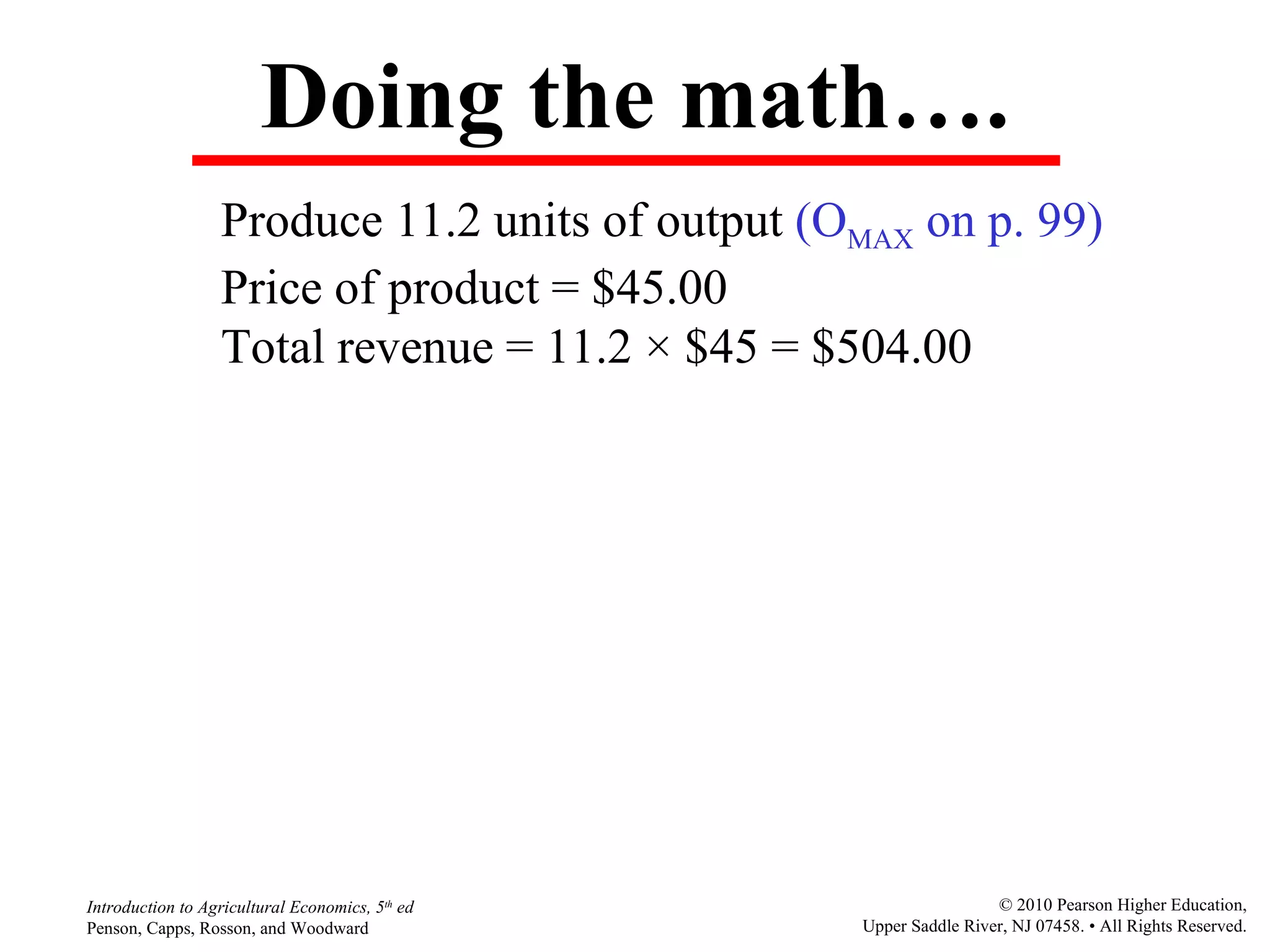
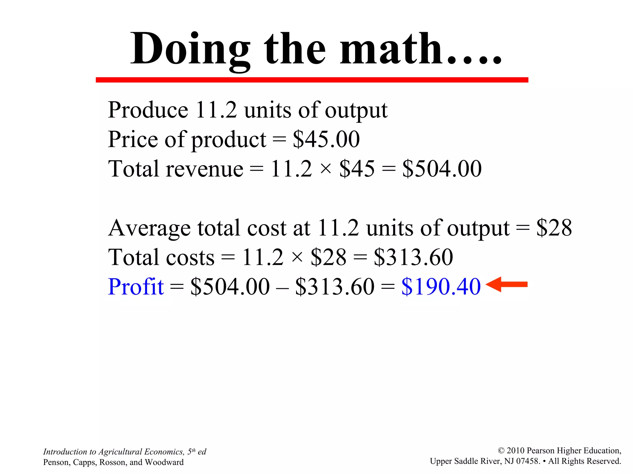
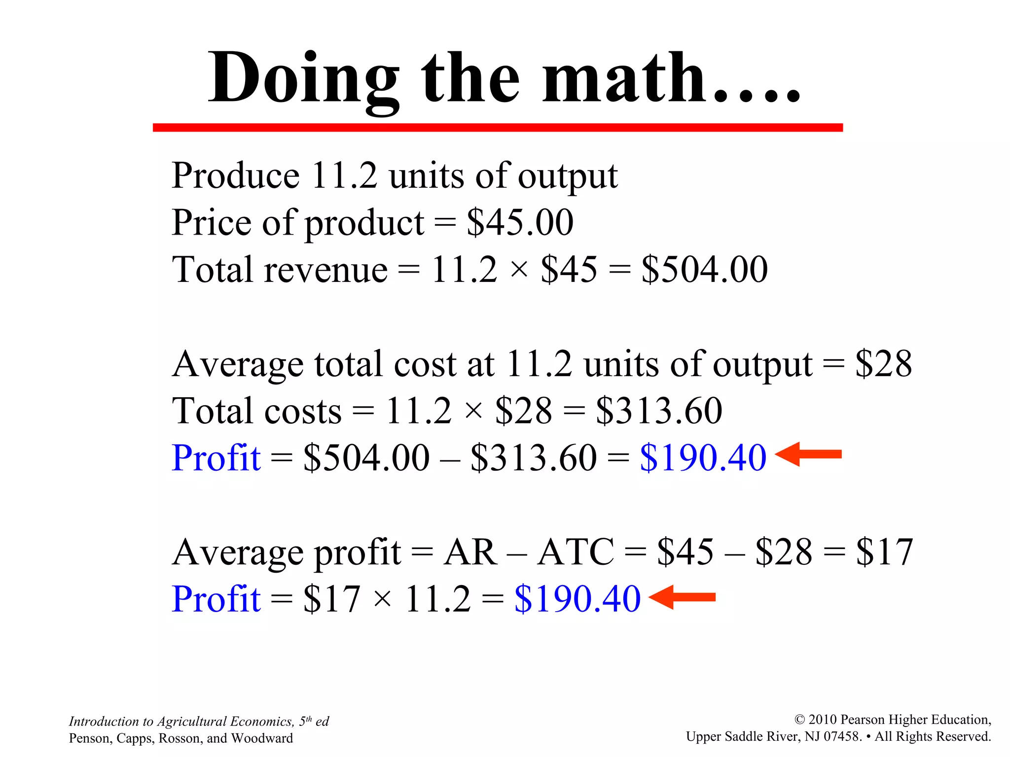
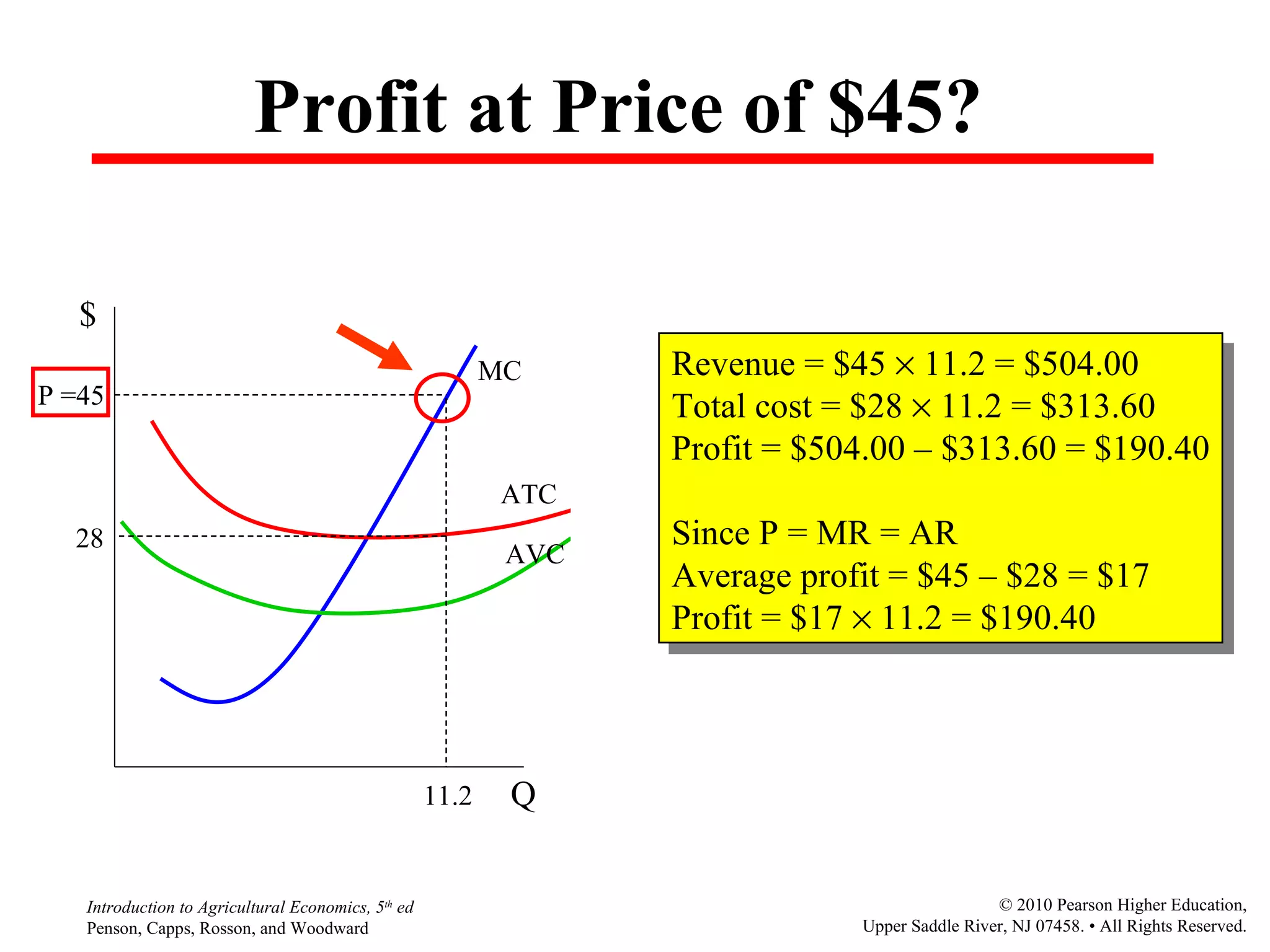
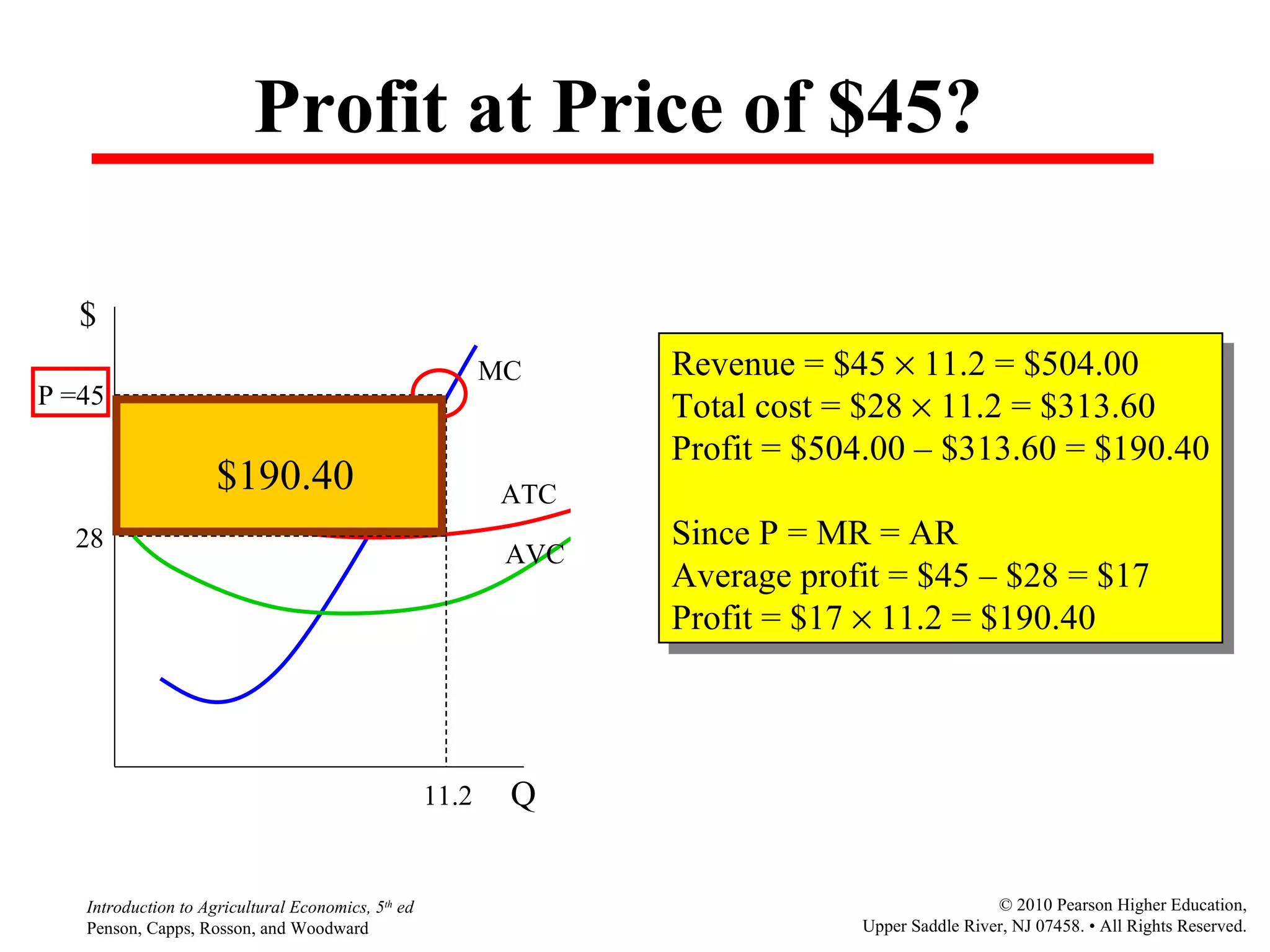
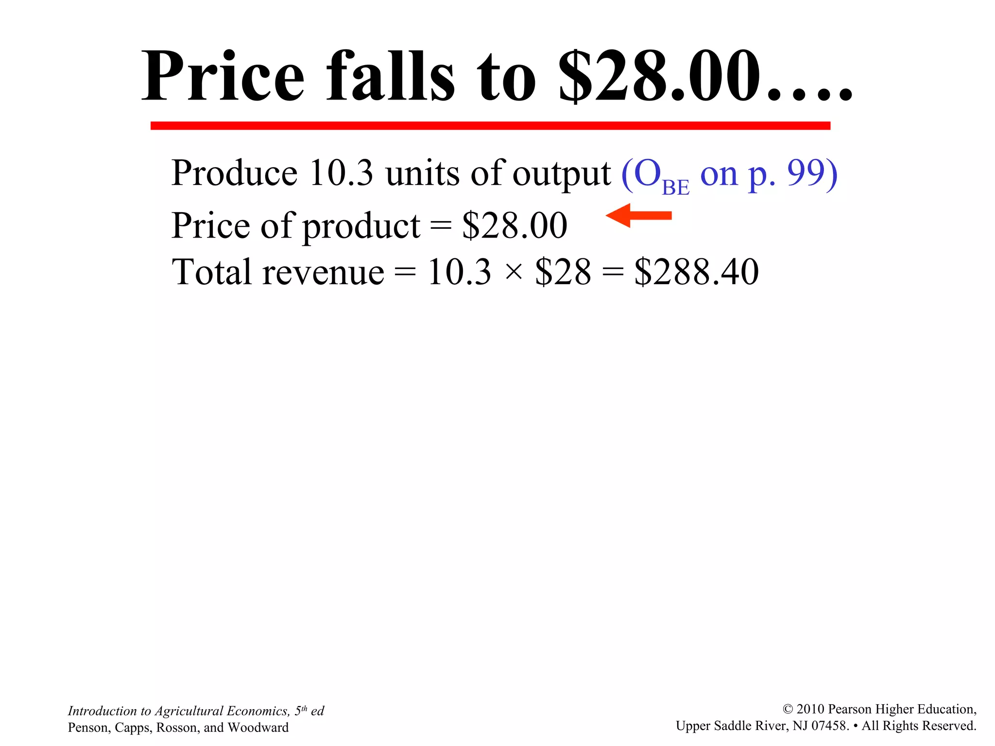
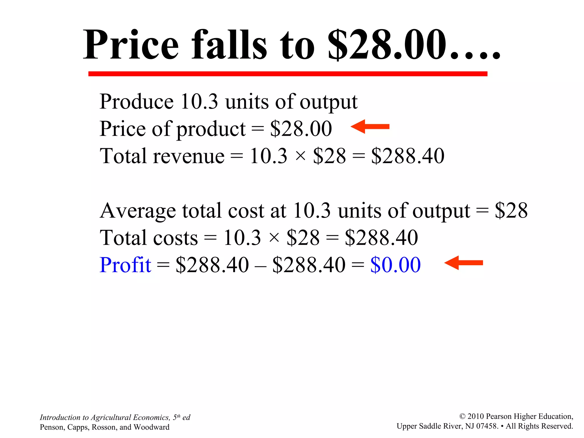
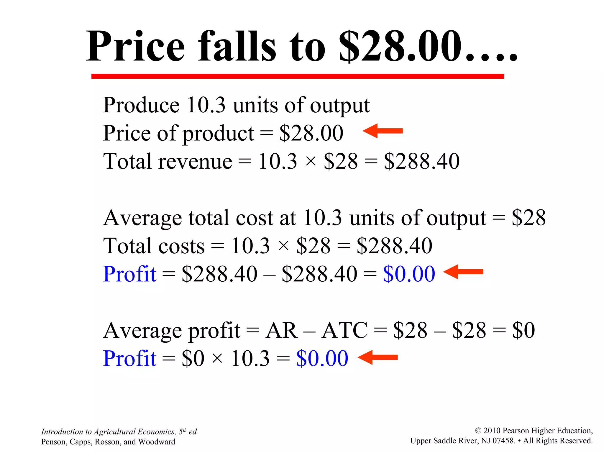
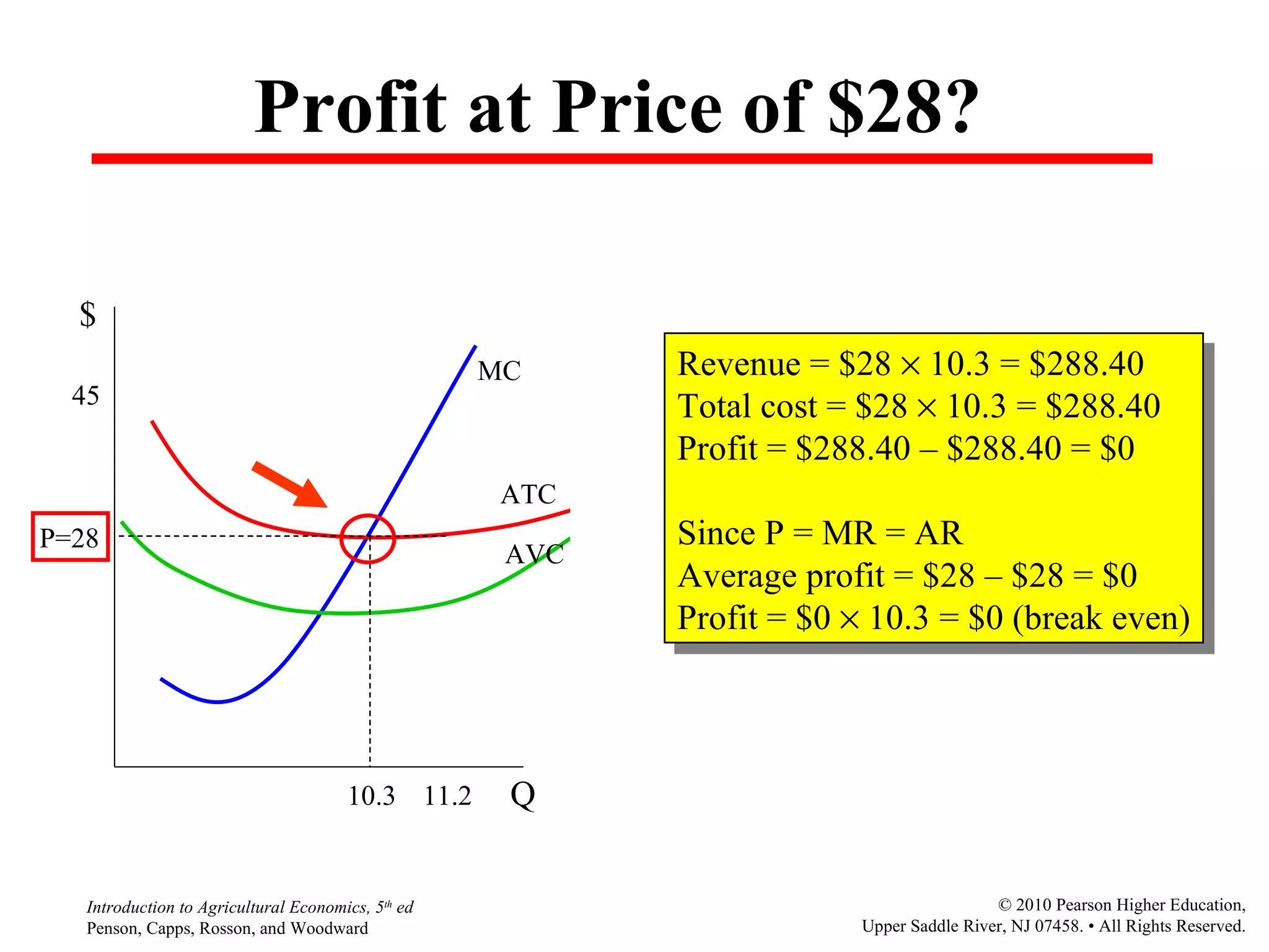
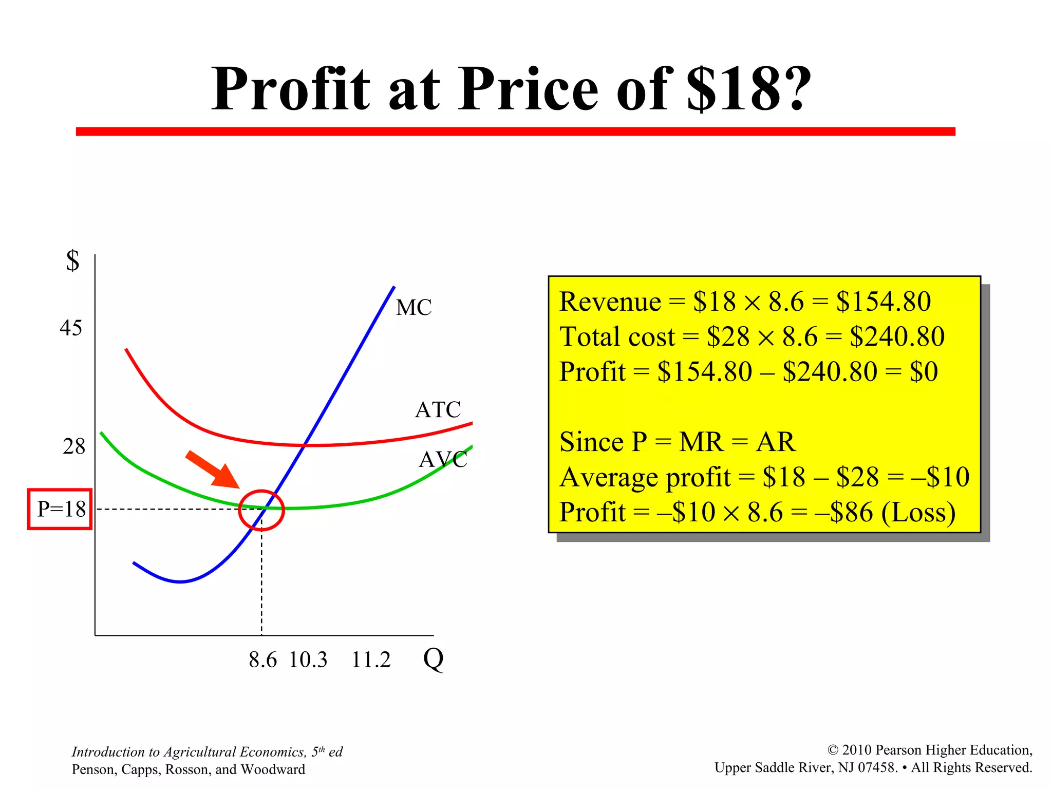
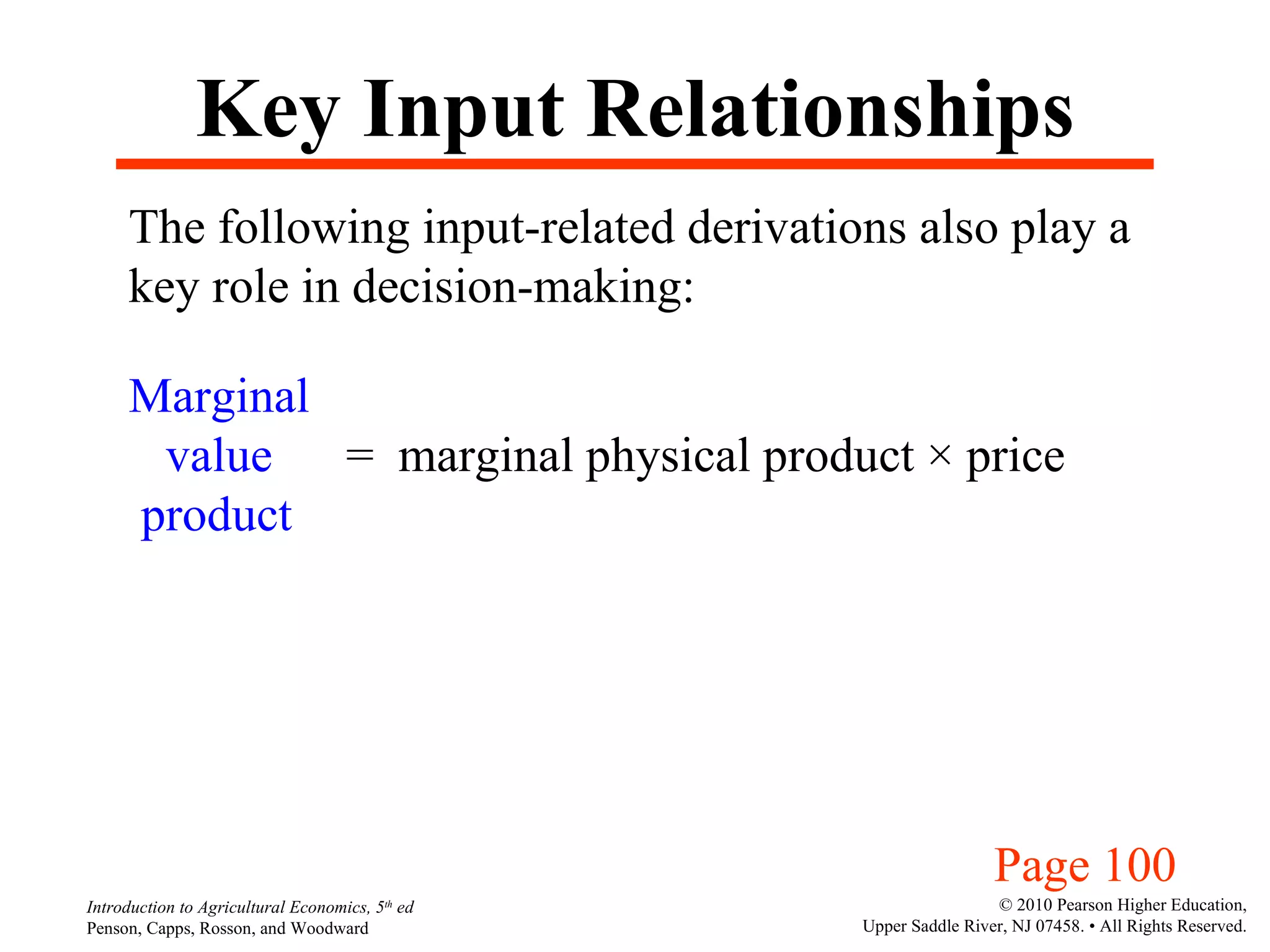
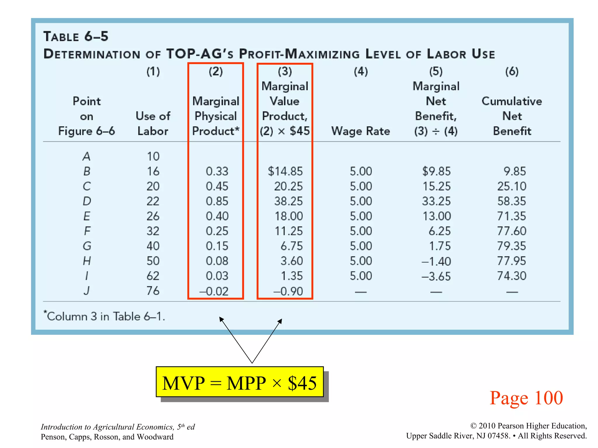
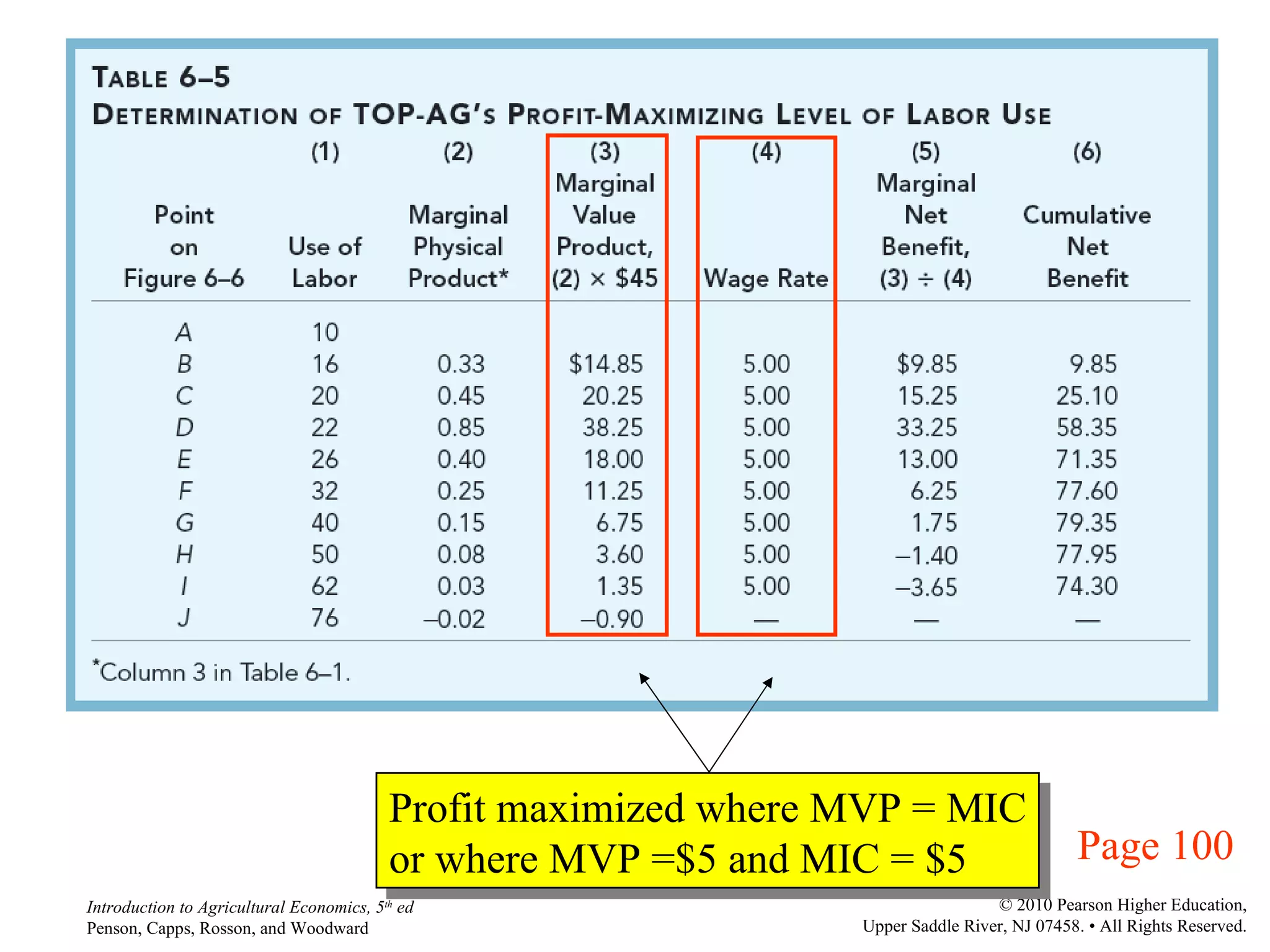
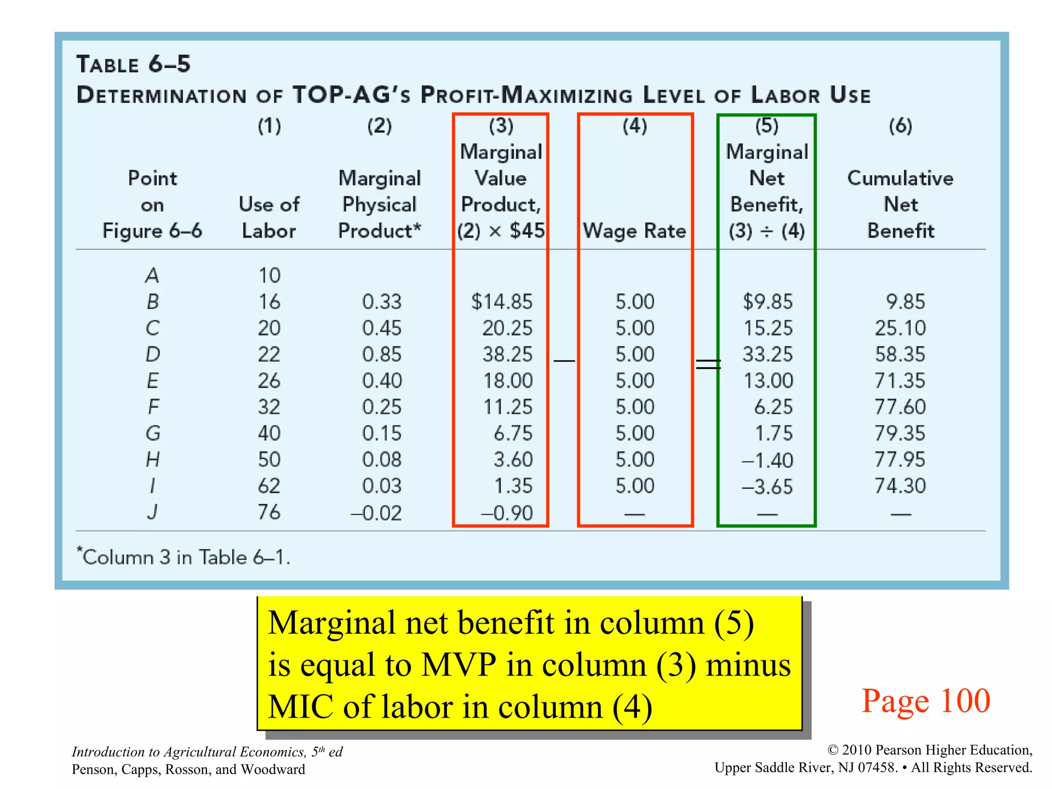
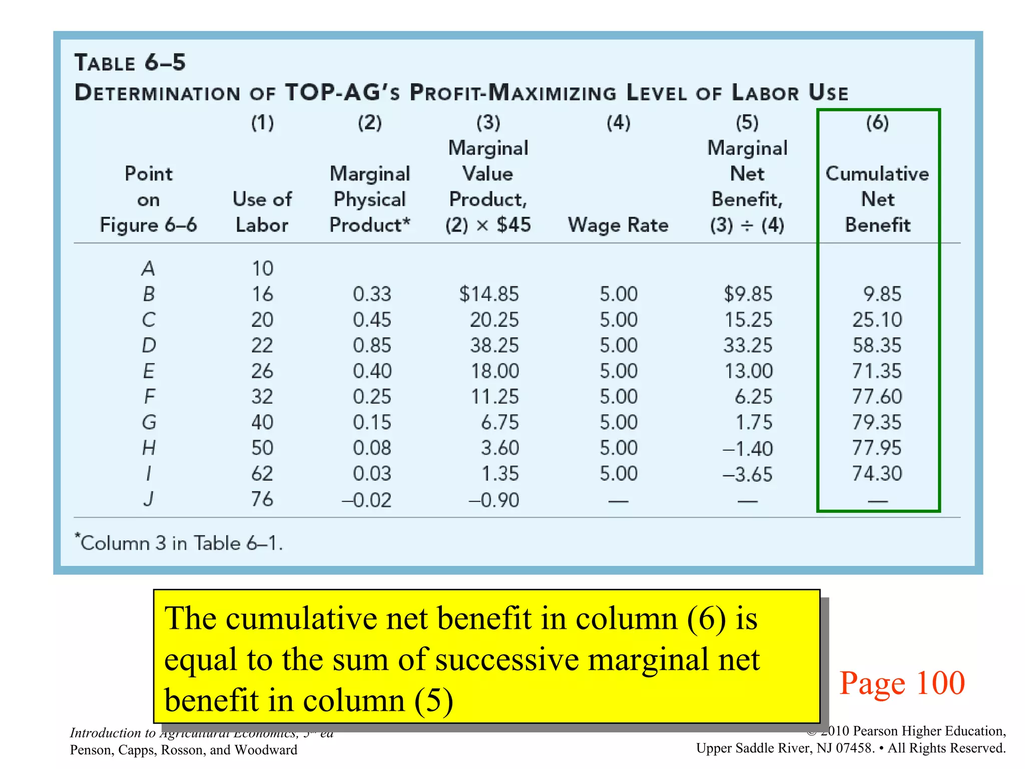
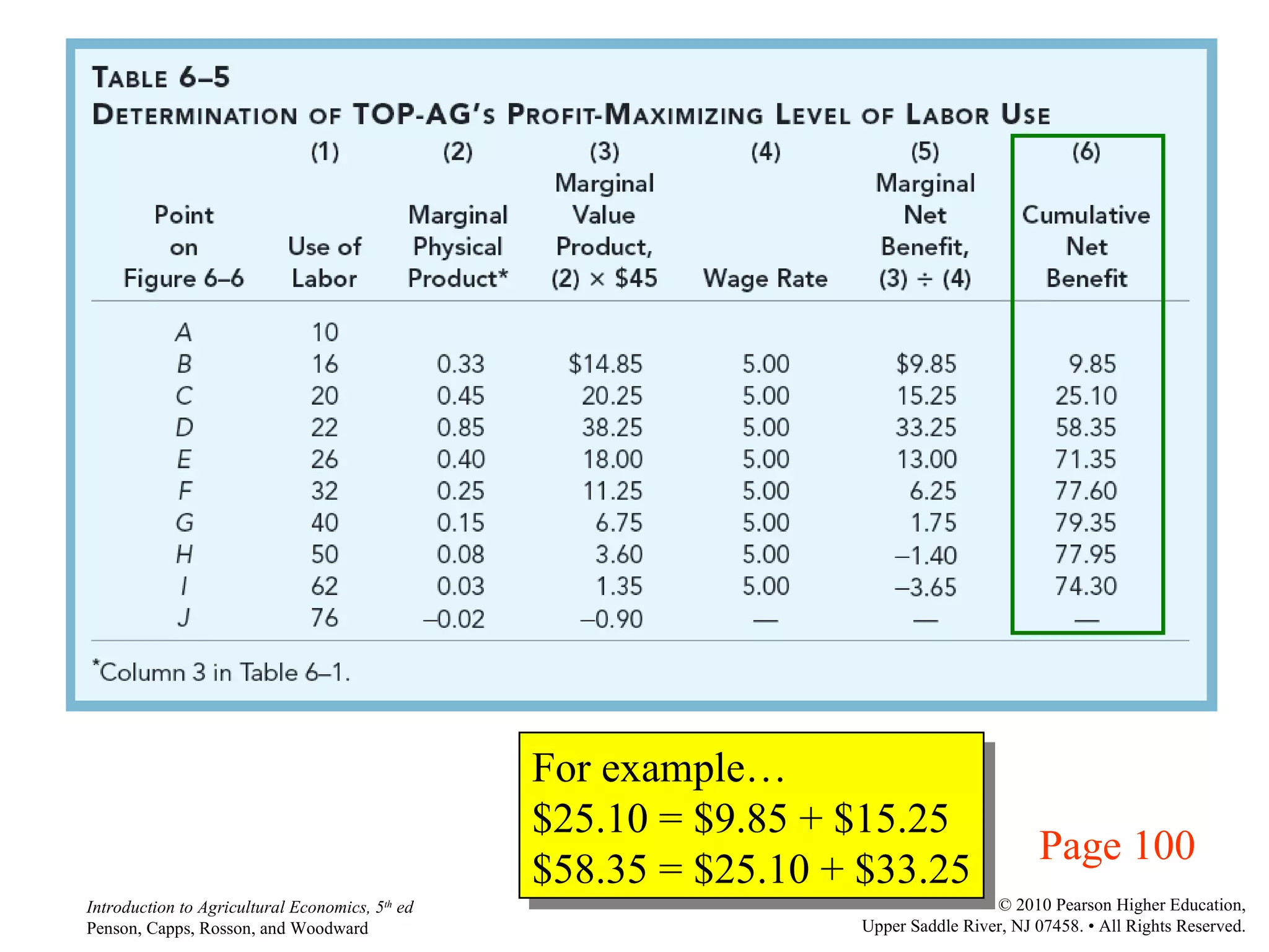
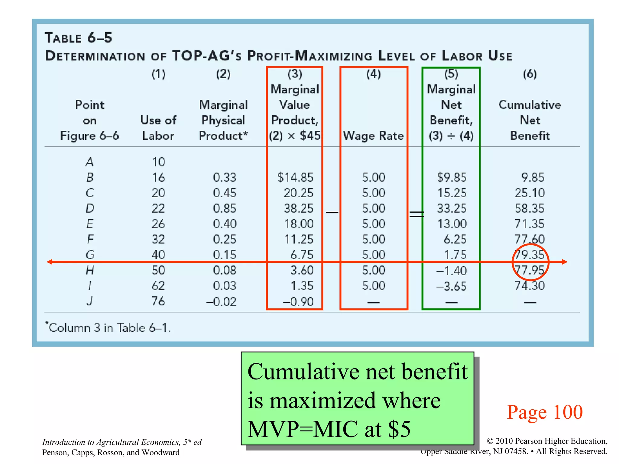
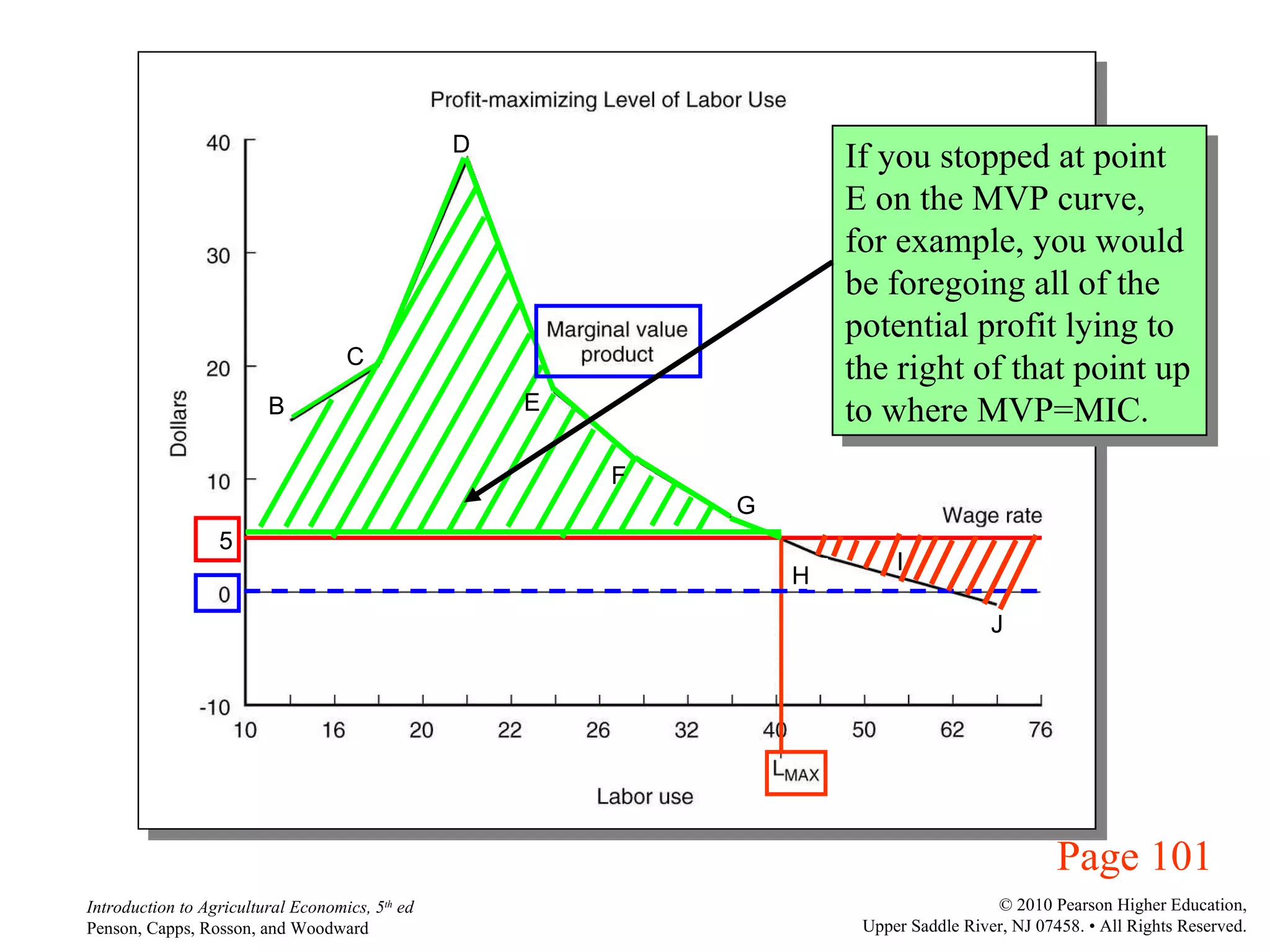
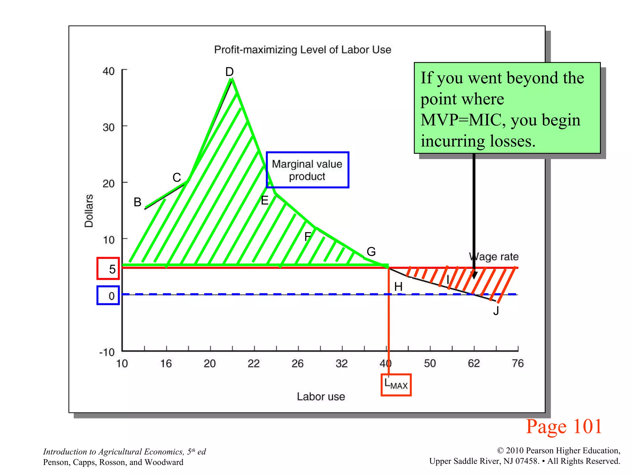
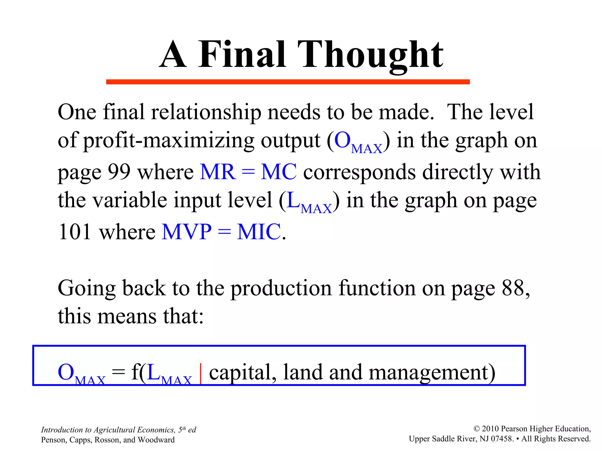
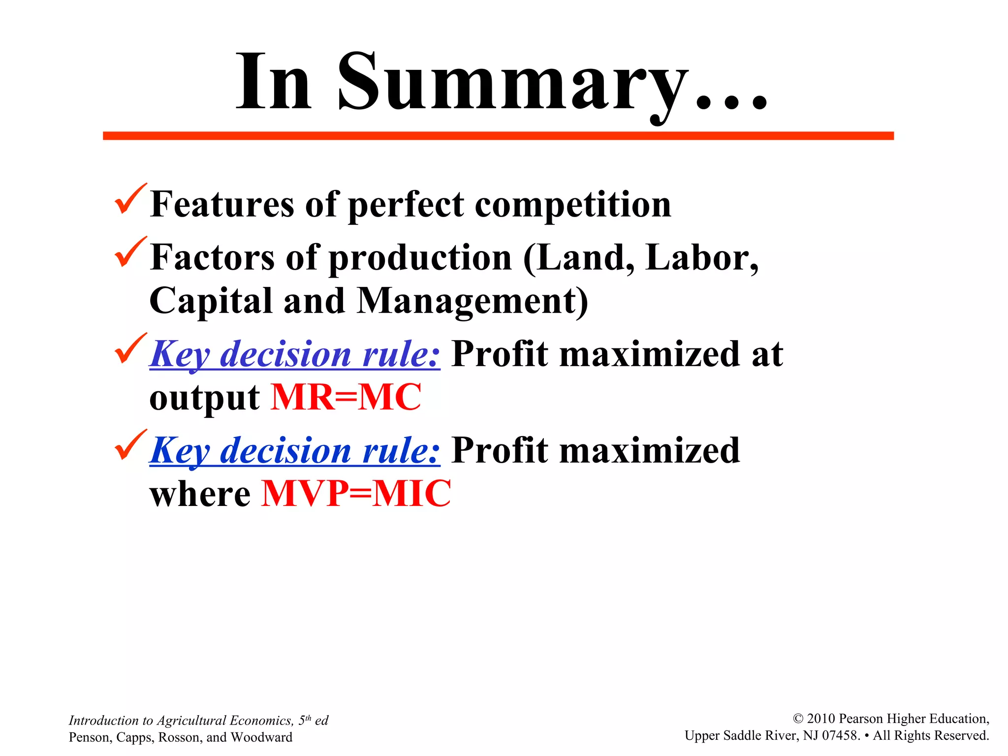
Agri 2312 chapter 6 introduction to production and resource use

Introduction to Production and Resource Use Chapter 6

Topics of Discussion Conditions of perfect competition Classification of inputs Important production relationships (assume one variable input in this chapter) Assessing short run business costs Economics of short run decisions

Conditions for Perfect Competition Homogeneous products No barriers to entry or exit Large number of sellers Perfect information Page 86

Classification of Inputs Land: includes renewable (forests) and non-renewable (minerals) resources Labor: all owner and hired labor services, excluding management Capital: manufactured goods such as fuel, chemicals, tractors and buildings Management: production decisions designed to achieve specific economic goal Pages 86-87

Production Function Output = f( labor | capital, land, and management) Start with one variable input Page 88

Production Function Output = f( labor | capital, land, and management) Start with one variable input assume all other inputs fixed at their current levels… Page 88

Coordinates of input and output on the TPP curve Page 89

Total Physical Product (TPP) Curve Variable input

Law of Diminishing Marginal Returns “ As successive units of a variable input are added to a production process with the other inputs held constant, the marginal physical product (MPP) eventually declines ” Page 93

Other Physical Relationships The following derivations of the TPP curve play An important role in decision-making: Marginal Physical =  Output ÷  Input Product Page 90

Other Physical Relationships The following derivations of the TPP curve play An important role in decision-making: Marginal Physical =  Output ÷  Input Product Average Physical = Output ÷ Input Product Pages 90-91

Change in output as you increase inputs Page 89

Total Physical Product (TPP) Curve  output  input Marginal physical product is .45 as labor is increased from 16 to 20 4.8 3

Output per unit input use

Total Physical Product (TPP) Curve output input Average physical product is .31 if labor use is 26

Plotting the MPP curve Page 91 Change in output associated with a change in inputs

Marginal Physcial Product Page 91 Change from point A to point B on the production function is an MPP of 0.33

Plotting the APP Curve Level of output divided by the level of input use

Average Physical Product Output divided by labor use is equal to 0.19

Three Stages of Production Average physical product (yield) is increasing in Stage I

Three Stages of Production Marginal physical product falls below the average physical product in Stage II

Three Stages of Production MPP goes negative as shown on Page 89…

Three Stages of Production Why are Stage I and Stage III irrational?

Three Stages of Production Productivity rising so why stop??? Output falling

Three Stages of Production The question therefore is where should I operate in Stage II? Page 114

Economic Dimension We need to account for the price of the product. We also need to account for the cost of the inputs. Total Cost of production is the costs associated with the use of all inputs Fixed costs Variable costs

Key Cost Relationships The following cost derivations play a key role in decision-making: Marginal cost =  total cost ÷  output Page 94-96

Key Cost Relationships The following cost derivations play a key role in decision-making: Marginal cost =  total cost ÷  output Average variable = total variable cost ÷ output cost Page 94-96

Key Cost Relationships The following cost derivations play a key role in decision-making: Marginal cost =  total cost ÷  output Average variable = total variable cost ÷ output cost Average total = total cost ÷ output cost Page 94-96

From TPP curve on page 89 Page 94

Fixed costs are $100 no matter the level of production Page 94

Column (2) divided by column (1) Page 94

Costs that vary with level of production

Column (4) divided by column (1)

Column (2) plus column (4)

Change in column (6) associated with a change in column (1)

Column (6) divided by column (1) or

or column (3) plus column (5)

Let’s graph the cost series in this table

Plotted cost relationships from table 6.3 on page 94 Page 95 O SD O BE Plotting costs for levels of output

Marginal and Average Revenue Marginal revenue = ∆ total revenue ÷ ∆ output

Now let’s assume this firm can sell its product for $45/unit

Key Revenue Concepts Notice the price in column (2) is identical to marginal revenue in column (7). What about average revenue, or AR? What do you see if you divide total revenue in column (3) by output in column (1)? Yes, $45. Thus, P = MR = AR under perfect competition. Page 98

Let’s see this in graphical form

Profit maximizing level of output, where MR=MC P=MR=AR $45 11.2

Average Profit = $17, or AR – ATC P=MR=AR $45-$28 $28

Grey area represents total economic profit if the price is $45… Page 99 P=MR=AR 11.2  ($45 - $28) = $190.40

Zero economic profit if price falls to P BE . Firm would only produce output O BE . AR-ATC=0 Page 99 P=MR=AR

Economic losses if price falls to P SD . Firm would shut down below output O SD Page 99 P=MR=AR

Where is the firm’s supply curve? Page 99 P=MR=AR

P=MR=AR Marginal cost curve above AVC curve?

Key Revenue Concepts Page 98 The previous graph indicated that profit is maximized at 11.2 units of output, where MR ($45) equals MC ($45). This occurs between lines G and H on the table above, where at 11.2 units of output profit would be $190.40 . Let’s do the math….

Doing the math…. Produce 11.2 units of output (O MAX on p. 99) Price of product = $45.00 Total revenue = 11.2 × $45 = $504.00

Doing the math…. Produce 11.2 units of output Price of product = $45.00 Total revenue = 11.2 × $45 = $504.00 Average total cost at 11.2 units of output = $28 Total costs = 11.2 × $28 = $313.60 Profit = $504.00 – $313.60 = $190.40

Doing the math…. Produce 11.2 units of output Price of product = $45.00 Total revenue = 11.2 × $45 = $504.00 Average total cost at 11.2 units of output = $28 Total costs = 11.2 × $28 = $313.60 Profit = $504.00 – $313.60 = $190.40 Average profit = AR – ATC = $45 – $28 = $17 Profit = $17 × 11.2 = $190.40

Profit at Price of $45? 28 P =45 $ Q 11.2 MC ATC AVC Revenue = $45  11.2 = $504.00 Total cost = $28  11.2 = $313.60 Profit = $504.00 – $313.60 = $190.40 Since P = MR = AR Average profit = $45 – $28 = $17 Profit = $17  11.2 = $190.40

Profit at Price of $45? 28 P =45 $ Q 11.2 MC ATC AVC Revenue = $45  11.2 = $504.00 Total cost = $28  11.2 = $313.60 Profit = $504.00 – $313.60 = $190.40 Since P = MR = AR Average profit = $45 – $28 = $17 Profit = $17  11.2 = $190.40 $190.40

Price falls to $28.00…. Produce 10.3 units of output (O BE on p. 99) Price of product = $28.00 Total revenue = 10.3 × $28 = $288.40

Price falls to $28.00…. Produce 10.3 units of output Price of product = $28.00 Total revenue = 10.3 × $28 = $288.40 Average total cost at 10.3 units of output = $28 Total costs = 10.3 × $28 = $288.40 Profit = $288.40 – $288.40 = $0.00

Price falls to $28.00…. Produce 10.3 units of output Price of product = $28.00 Total revenue = 10.3 × $28 = $288.40 Average total cost at 10.3 units of output = $28 Total costs = 10.3 × $28 = $288.40 Profit = $288.40 – $288.40 = $0.00 Average profit = AR – ATC = $28 – $28 = $0 Profit = $0 × 10.3 = $0.00

Profit at Price of $28? P=28 45 $ Q 11.2 10.3 MC ATC AVC Revenue = $28  10.3 = $288.40 Total cost = $28  10.3 = $288.40 Profit = $288.40 – $288.40 = $0 Since P = MR = AR Average profit = $28 – $28 = $0 Profit = $0  10.3 = $0 (break even)

Price falls to $18.00…. Produce 8.6 units of output (O SD on p. 99) Price of product = $18.00 Total revenue = 8.6 × $18 = $154.80

Price falls to $18.00…. Produce 8.6 units of output Price of product = $18.00 Total revenue = 8.6 × $18 = $154.80 Average total cost at 8.6 units of output = $28 Total costs = 8.6 × $28 = $240.80 Profit = $154.80 – $240.80 = – $86.00

Price falls to $18.00…. Produce 8.6 units of output Price of product = $18.00 Total revenue = 8.6 × $18 = $154.80 Average total cost at 8.6 units of output = $28 Total costs = 8.6 × $28 = $240.80 Profit = $154.80 – $240.80 = – $86.00 Average profit = AR – ATC = $18 – $28 = – $10 Profit = – $10 × 8.6 = – $86.00

Profit at Price of $18? 28 P=18 45 $ Q 11.2 10.3 8.6 MC ATC AVC Revenue = $18  8.6 = $154.80 Total cost = $28  8.6 = $240.80 Profit = $154.80 – $240.80 = $0 Since P = MR = AR Average profit = $18 – $28 = – $10 Profit = – $10  8.6 = – $86 (Loss)

Price falls to $10.00…. Produce 7.0 units of output (below O SD on p. 99) Price of product = $10.00 Total revenue = 7.0 × $10 = $70.00

Price falls to $10.00…. Produce 7.0 units of output Price of product = $10.00 Total revenue = 7.0 × $10 = $70.00 Average total cost at 7.0 units of output = $28 Total costs = 7.0 × $28 = $196.00 Profit = $70.00 – $196.00 = – $126.00

Price falls to $10.00…. Produce 7.0 units of output Price of product = $10.00 Total revenue = 7.0 × $10 = $70.00 Average total cost at 7.0 units of output = $30 Total costs = 7.0 × $30 = $210.00 Profit = $70.00 – $210.00 = – $140.00 Average variable costs = $19 Total variable costs = $19 × 7.0 = $133.00 Revenue – variable costs = –$63.00 !!!!!

Profit at Price of $10? 28 P=10 18 45 $ Q 11.2 10.3 8.6 MC ATC AVC 7.0 Revenue = $10  7.0 = $70.00 Total cost = $30  7.0 = $210.00 Profit = $70.00 – $210.00 = $140.00 Since P = MR = AR Average profit = $10 – $30 = – $20 Profit = – $20  7.0 = – $140 Average variable cost = $19 Variable costs = $19  7.0 = $133.00 Revenue – variable costs = – $63 Not covering variable costs!!!!!!

The Firm’s Supply Curve 28 P=10 18 45 $ Q 11.2 10.3 8.6 MC ATC AVC 7.0

Now let’s look at the demand for a single input: Labor

Key Input Relationships The following input-related derivations also play a key role in decision-making: Marginal value = marginal physical product × price product Page 100

Key Input Relationships The following input-related derivations also play a key role in decision-making: Marginal value = marginal physical product × price product Marginal input = wage rate, rental rate, etc. cost Page 100

5 B C D E F G H I J Wage rate represents the MIC for labor

5 B C D E F G H I J Use a variable input like labor up to the point where the value received from the market equals the cost of another unit of input, or MVP=MIC

5 The area below the green lined MVP curve and above the green lined MIC curve represents cumulative net benefit. B C D E F G H I J

Profit maximized where MVP = MIC or where MVP =$5 and MIC = $5

Marginal net benefit in column (5) is equal to MVP in column (3) minus MIC of labor in column (4) = –

The cumulative net benefit in column (6) is equal to the sum of successive marginal net benefit in column (5)

For example… $25.10 = $9.85 + $15.25 $58.35 = $25.10 + $33.25

= – Cumulative net benefit is maximized where MVP=MIC at $5

5 If you stopped at point E on the MVP curve, for example, you would be foregoing all of the potential profit lying to the right of that point up to where MVP=MIC. B C D E F G H I J

5 If you went beyond the point where MVP=MIC, you begin incurring losses. B C D E F G H I J

A Final Thought One final relationship needs to be made. The level of profit-maximizing output ( O MAX ) in the graph on page 99 where MR = MC corresponds directly with the variable input level ( L MAX ) in the graph on page 101 where MVP = MIC . Going back to the production function on page 88, this means that: O MAX = f( L MAX | capital, land and management)

In Summary… Features of perfect competition Factors of production (Land, Labor, Capital and Management) Key decision rule: Profit maximized at output MR=MC Key decision rule: Profit maximized where MVP=MIC

Chapter 7 focuses on the choice of inputs to use and products to produce ….

Agri 2312 chapter 6 introduction to production and resource use

More Related Content

What's hot

Similar to Agri 2312 chapter 6 introduction to production and resource use

More from Rita Conley

Recently uploaded

Agri 2312 chapter 6 introduction to production and resource use