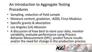
Aggregate Testing 101
James Cox – Cemex
Jennifer Hanley – Gilson Company
PRESENTE
R’S
LOGO
An introduction to Aggregate Testing
Procedures
• Sampling, reduction of field sample
• Moisture content, gradation, -#200, Finus Modulus
• Specific gravity & absorption
• Los Angeles (LA) Abrasion
• A discussion of how best to store your data, monitor
variability, evaluate performance using Process
Behavior Measurement (SPC), predict future results
and/or the need for change in the production process.
Aggregate Testing Procedures
• DOT-Department of Transportation
• ASTM-American Society of Testing and Materials
• AASHTO-American Association of State Highway
Transportation Officials
Maximum & Nominal Size
Amounts Finer than Each Laboratory Sieve (Square Openings), % Weight
Size
Number
Nominal Size, Square
Openings
4-in
(100-
mm)
3 1/2-in
(90-mm)
3-in
(75-
mm)
2 1/2-in
(63-mm)
2-in
(50-mm)
1 1/2-in
(37.5-mm)
1-in
(25.0-mm)
3/4-in
(19.0-mm)
1/2-in
(12.5-mm)
3/8-in
(9.5-mm)
No.4
(4.75-mm)
N0.8
(2.36-
mm)
No.16
(1.18-
mm)
No.50
(0.300-
mm)
No.100
(0.150-
mm)
1 3 1/2 to 1 1/2-in
(90 to 37.5-mm)
100 90 to 100 … 25 to 60 … 0 to 15 … 0 to 5 … … … … … … …
2 2 1/2 to 1 1/2-in
(63 to 37.5-mm)
… … 100 90 to 100 35 to 70 0 to 15 … 0 to 5 … … … … … … …
24 2 1/2 to 3/4-in
(63 to 19.0-mm)
… … 100 90 to 100 … 25 to 60 … 0 to 10 0 to 5 … … … … … …
3 2 to 1-in
(50 to 25.0-mm)
… … … 100 90 to 100 35 to 70 0 to 15 … 0 to 5 … … … … … …
357 2-in to N0.4
(50 to 4.75-mm)
… … … 100 95 to 100 … 35 to 70 … 10 to 30 … 0 to 5 … … … …
4 1 1/2 to 3/4-in
(37.5 to 19.0-mm)
… … … … 100 90 to 100 20 to 55 0 to 15 … 0 to 5 … … … … …
467 1 1/2-in to No.4
(37.5 to 4.75-mm)
… … … … 100 95 to 100 … 35 to 70 … 10 to 30 0 to 5 … … … …
5 1 to 1/2-in
(25.0 to 12.5-mm)
… … … … … 100 90 to 100 20 to 55 0 to 10 0 to 5 … … … … …
56 1 to 3/8-in
(25.0 to 9.5-mm)
… … … … … 100 90 to 100 40 to 85 10 to 40 0 to 15 0 to 5 … … … …
57 1-in to No.4
(25.0 to 4.75-mm)
… … … … … 100 95 to 100 … 25 to 60 … 0 to 10 0 to 5 … … …
6 3/4 to 3/8-in
(19.0 to 9.5-mm)
… … … … … … 100 90 to 100 20 to 55 0 to 15 0 to 5 … … … …
67 3/4-in to No.4
(19.0 to 4.75-mm)
… … … … … … 100 90 to 100 … 20 to 55 0 to 10 0 to 5 … … …
68 3/4-in to No.8
(19.0 to 2.36-mm)
… … … … … … 100 90 to 100 … 30 to 65 5 to 25 0 to 10 0 to 5 … …
7 1/2-in to No.4
(12.5 to 4.75-mm)
… … … … … … … 100 90 to 100 40 to 70 0 to 15 0 to 5 … … …
78 1/2-in to No.8
(12.5 to 2.36-mm)
… … … … … … … 100 90 to 100 40 to 75 5 to 25 0 to 10 0 to 5 … …
8 3/8-in to No.4
(9.5 to 2.36-mm)
… … … … … … … … 100 85 to 100 10 to 30 0 to 10 0 to 5 … …
89 3/8-in to No.16
(9.5 to 1.18-mm)
… … … … … … … … 100 90 to 100 20 to 55 5 to 30 0 to 10 0 to 5 …
9 N0.4 to No.16
(4.75 to 1.18-mm)
… … … … … … … … … 100 85 to 100 10 to 40 0 to 10 0 to 5 …
10 No.4 to 0*
(4.75-mm)
… … … … … … … … … 100 85 to 100 … … … 10 to 30
*Screenings From ASTM D 448
It All Starts with Sampling
• Properly trained personnel
• Develop a plan agreeable by all parties
• Use power equipment if you have it
• Field sample size is important
ASTM D 75, AASHTO T 2
Minimum Field Sample Size
• Based on Nominal Maximum size:
– 4 Stone 1 ½” 75lb
– 57 Stone 1” 50lb
– 67 Stone ¾” 25lb
– 89 Stone 3/8” 10lb
– Fine Agg -#4mesh 10lb
ASTM D 75, AASHTO T 2
Reducing Field Sample to Testing
Size
• Split down to obtain required minimum test
sample size
ASTM C 702, AASHTO R 76
Gradation
• Fine aggregate
– Most particles smaller than #4 (4.75mm)
• Coarse Aggregate
– Most particles larger than #4 (2.75mm)
• Mixed/Dense graded aggregate
– Combination of fine & coarse, base courses
Sieve Analysis of Fine & Coarse
Aggregate
ASTM C 136, AASHTO T 127
Sieve Analysis of Fine & Coarse
Aggregate
• Why some sieves in inches and others #?
• Sieve sizes are based on
dimensions of the mesh size
opening or the number of
openings per linear inch
ASTM E 11
Sieve Analysis of Fine & Coarse
Aggregate
Sieve Analysis
Sieve Analysis
Sieve Analysis
Ind % Retained = 100 X Mass Retained ÷ Dry
Mass
Sieve Analysis
Add up successive Ind % Retained to obtain Cumulative %
Retained
Sieve Analysis
% Passing = 100 – Cumulative % Retained
Sieve Analysis
Sieve Analysis
Individual % Retained
Cumulative % Retained
Cumulative % Passing
Total Moisture Content
• Weigh wet sample
• Dry to constant mass @ 110 +/- 5C, 230 +/- 9F
• Weigh dry sample
% moisture = 100 × (Wet Wt. – Dry Wt.) ÷ Dry Wt.
= 100 x Weight of Water ÷ Dry Wt.
ASTM C 566 , AASHTO T 255
Total Moisture Content
% moisture = 100 x Weight of Water ÷ Dry Wt.
Solids
Water
Air
Materials Finer than the 75µm (No
200) Sieve in Mineral Aggregates
by Washing ASTM C 117, AASHTO T 11
• Minimum sample size:
(based on Nominal Maximum size)
– 1 ½” 5000g
– ¾” 2500g
– 3/8” 1000g
– #4mesh 500g
– #8mesh 100g
Materials Finer than the 75µm
(No 200) Sieve in Mineral
Aggregates by Washing
ASTM C 117, AASHTO T 11
Materials Finer than the 75µm
(No 200) Sieve in Mineral
Aggregates by Washing
ASTM C 117, AASHTO T 11
%-#200 = [(original dry mass – dry mass
after washing) ÷ original dry mass] X 100
%-#200 = (loss ÷ original dry mass) X 100
Finus Modulus (FM)
• Index which indicates fineness
• Sum of cumulative % retained on specified
sieves divided by 100 Specified Sieves
3/8
#4
8
16
30
50
100
FM = 242.2 ÷ 100 = 2.42
Specific Gravity & Absorption
• Coarse • Fine
Fine ASTM C 128, AASHTO T 84
Coarse ASTM C 127, AASHTO T 85
Ratio of the density of one material to a reference material
Specific Gravity & Absorption
• Coarse
Specific Gravity & Absorption
• Coarse
Specific Gravity & Absorption
• Dry Bulk Specific Gravity
oven dry wt.
SSD wt. – SSD in H2O wt.
• Saturated Surface Dry Specific Gravity
SSD wt.
SSD wt. – SSD in H2O wt.
Oven Dry
SSD
Specific Gravity & Absorption
SSD
• Fine
Specific Gravity & Absorption
• Absorption, %
SSD wt. - oven dry wt.
oven dry wt.
Los Angeles Abrasion
• Specified grading of
sample is placed into
the apparatus along
with a charge of steel
spheres and rotated a
specified # of times
ASTM C 131, AASHTO T 96
Los Angeles Abrasion
% Loss = 100 X (wt. original sample – wt. retained on #12
sieve)
wt. original sample
% Loss = 100 X (material passing the #12 sieve)
wt. original sample
Comparison
Florida Limestone Georgia Granite
Specific Gravity (SSD) 2.490 2.678
Absorption (%) 5.0 0.2
LA Abrasion 32 21
Collecting, Analyzing & Storing Data
• Data validation upon entry
• Realtime, share across network
• Ease of calculations
• Less errors
• Standardized worksheets
• Rapid analysis
• Automation of reporting & alerts
Data Validation
Feed Back
Analyzing Data
• Mean, average (X)
• Standard Deviation, square root of the variance
Standard Deviation
Standard Deviation
Standard Deviation
Standard Deviation
Essentially the standard deviation is the
average distance of each measurement
from the mean of all those measurements
Standard Deviation
Process Behavior Measurement
Mean
Mean
Process Behavior Measurement
Spec.,
Voice of
the
Custome
r
Elbow room
QC
“There is a very abrupt change in the
production # 57 samples today …
gave us a signal on the process
behavior chart. Did we do anything
to cause this change yesterday after
plant shut down?” That’s a signal!
Maintenance
“We found E6X20 T/D # 1,2 screens with
3/4" instead of 1-1/8". Now is back to 1-1/8"
p/p screens.”
A missed signal is an wasted opportunity!
QC
“You don’t have to know my plant you
just have to listen to the signals”
Process Behavior Measurement
Feed Back
Analysis
Analysis
Automated Notifications
Automated Reports
• Preconfigured
• Generated when you want
• Hourly
• Daily
• Monthly
• emailed
• Report or link
• Available anytime in app
Automated Reports
Automated Reports
Automated Reports
Automated Reports
Auto
Evaluation
• Gives you
feedback
• With supporting
graphics
• Only generates
for exceptions
• No reviewing
non problem
data/products
Advantages of a Database
• Ease of data entry
• Data entry validation
• Visual feedback on results
• On line, real time
• Built in analysis tools
• Automated email alerts
• Automated reporting
• Auto analysis of data
Summary
• Sampling is important (Job #1)
• Remember minimum sample sizes
– Samples & Tests
• There are databases available for data entry
and evaluation
o Data entry validation
o Visual feedback on results
o Automated email alerts
o Automated reporting
o Auto analysis of data
Questions?
References
• ASTM ASTM.org
• AASHTO transportation.org
• ACI Concrete.org
• NRMCA nrmca.org
• NAPA asphaltpavement.org
• Understanding SPC Donald J. Wheeler
SPCPress.com

Aggregate testing

  • 2.
    Aggregate Testing 101 JamesCox – Cemex Jennifer Hanley – Gilson Company PRESENTE R’S LOGO
  • 3.
    An introduction toAggregate Testing Procedures • Sampling, reduction of field sample • Moisture content, gradation, -#200, Finus Modulus • Specific gravity & absorption • Los Angeles (LA) Abrasion • A discussion of how best to store your data, monitor variability, evaluate performance using Process Behavior Measurement (SPC), predict future results and/or the need for change in the production process.
  • 4.
    Aggregate Testing Procedures •DOT-Department of Transportation • ASTM-American Society of Testing and Materials • AASHTO-American Association of State Highway Transportation Officials
  • 5.
    Maximum & NominalSize Amounts Finer than Each Laboratory Sieve (Square Openings), % Weight Size Number Nominal Size, Square Openings 4-in (100- mm) 3 1/2-in (90-mm) 3-in (75- mm) 2 1/2-in (63-mm) 2-in (50-mm) 1 1/2-in (37.5-mm) 1-in (25.0-mm) 3/4-in (19.0-mm) 1/2-in (12.5-mm) 3/8-in (9.5-mm) No.4 (4.75-mm) N0.8 (2.36- mm) No.16 (1.18- mm) No.50 (0.300- mm) No.100 (0.150- mm) 1 3 1/2 to 1 1/2-in (90 to 37.5-mm) 100 90 to 100 … 25 to 60 … 0 to 15 … 0 to 5 … … … … … … … 2 2 1/2 to 1 1/2-in (63 to 37.5-mm) … … 100 90 to 100 35 to 70 0 to 15 … 0 to 5 … … … … … … … 24 2 1/2 to 3/4-in (63 to 19.0-mm) … … 100 90 to 100 … 25 to 60 … 0 to 10 0 to 5 … … … … … … 3 2 to 1-in (50 to 25.0-mm) … … … 100 90 to 100 35 to 70 0 to 15 … 0 to 5 … … … … … … 357 2-in to N0.4 (50 to 4.75-mm) … … … 100 95 to 100 … 35 to 70 … 10 to 30 … 0 to 5 … … … … 4 1 1/2 to 3/4-in (37.5 to 19.0-mm) … … … … 100 90 to 100 20 to 55 0 to 15 … 0 to 5 … … … … … 467 1 1/2-in to No.4 (37.5 to 4.75-mm) … … … … 100 95 to 100 … 35 to 70 … 10 to 30 0 to 5 … … … … 5 1 to 1/2-in (25.0 to 12.5-mm) … … … … … 100 90 to 100 20 to 55 0 to 10 0 to 5 … … … … … 56 1 to 3/8-in (25.0 to 9.5-mm) … … … … … 100 90 to 100 40 to 85 10 to 40 0 to 15 0 to 5 … … … … 57 1-in to No.4 (25.0 to 4.75-mm) … … … … … 100 95 to 100 … 25 to 60 … 0 to 10 0 to 5 … … … 6 3/4 to 3/8-in (19.0 to 9.5-mm) … … … … … … 100 90 to 100 20 to 55 0 to 15 0 to 5 … … … … 67 3/4-in to No.4 (19.0 to 4.75-mm) … … … … … … 100 90 to 100 … 20 to 55 0 to 10 0 to 5 … … … 68 3/4-in to No.8 (19.0 to 2.36-mm) … … … … … … 100 90 to 100 … 30 to 65 5 to 25 0 to 10 0 to 5 … … 7 1/2-in to No.4 (12.5 to 4.75-mm) … … … … … … … 100 90 to 100 40 to 70 0 to 15 0 to 5 … … … 78 1/2-in to No.8 (12.5 to 2.36-mm) … … … … … … … 100 90 to 100 40 to 75 5 to 25 0 to 10 0 to 5 … … 8 3/8-in to No.4 (9.5 to 2.36-mm) … … … … … … … … 100 85 to 100 10 to 30 0 to 10 0 to 5 … … 89 3/8-in to No.16 (9.5 to 1.18-mm) … … … … … … … … 100 90 to 100 20 to 55 5 to 30 0 to 10 0 to 5 … 9 N0.4 to No.16 (4.75 to 1.18-mm) … … … … … … … … … 100 85 to 100 10 to 40 0 to 10 0 to 5 … 10 No.4 to 0* (4.75-mm) … … … … … … … … … 100 85 to 100 … … … 10 to 30 *Screenings From ASTM D 448
  • 6.
    It All Startswith Sampling • Properly trained personnel • Develop a plan agreeable by all parties • Use power equipment if you have it • Field sample size is important ASTM D 75, AASHTO T 2
  • 7.
    Minimum Field SampleSize • Based on Nominal Maximum size: – 4 Stone 1 ½” 75lb – 57 Stone 1” 50lb – 67 Stone ¾” 25lb – 89 Stone 3/8” 10lb – Fine Agg -#4mesh 10lb ASTM D 75, AASHTO T 2
  • 8.
    Reducing Field Sampleto Testing Size • Split down to obtain required minimum test sample size ASTM C 702, AASHTO R 76
  • 9.
    Gradation • Fine aggregate –Most particles smaller than #4 (4.75mm) • Coarse Aggregate – Most particles larger than #4 (2.75mm) • Mixed/Dense graded aggregate – Combination of fine & coarse, base courses
  • 10.
    Sieve Analysis ofFine & Coarse Aggregate ASTM C 136, AASHTO T 127
  • 11.
    Sieve Analysis ofFine & Coarse Aggregate • Why some sieves in inches and others #? • Sieve sizes are based on dimensions of the mesh size opening or the number of openings per linear inch ASTM E 11
  • 12.
    Sieve Analysis ofFine & Coarse Aggregate
  • 13.
  • 14.
  • 15.
    Sieve Analysis Ind %Retained = 100 X Mass Retained ÷ Dry Mass
  • 16.
    Sieve Analysis Add upsuccessive Ind % Retained to obtain Cumulative % Retained
  • 17.
    Sieve Analysis % Passing= 100 – Cumulative % Retained
  • 18.
  • 19.
    Sieve Analysis Individual %Retained Cumulative % Retained Cumulative % Passing
  • 20.
    Total Moisture Content •Weigh wet sample • Dry to constant mass @ 110 +/- 5C, 230 +/- 9F • Weigh dry sample % moisture = 100 × (Wet Wt. – Dry Wt.) ÷ Dry Wt. = 100 x Weight of Water ÷ Dry Wt. ASTM C 566 , AASHTO T 255
  • 21.
    Total Moisture Content %moisture = 100 x Weight of Water ÷ Dry Wt. Solids Water Air
  • 22.
    Materials Finer thanthe 75µm (No 200) Sieve in Mineral Aggregates by Washing ASTM C 117, AASHTO T 11 • Minimum sample size: (based on Nominal Maximum size) – 1 ½” 5000g – ¾” 2500g – 3/8” 1000g – #4mesh 500g – #8mesh 100g
  • 23.
    Materials Finer thanthe 75µm (No 200) Sieve in Mineral Aggregates by Washing ASTM C 117, AASHTO T 11
  • 24.
    Materials Finer thanthe 75µm (No 200) Sieve in Mineral Aggregates by Washing ASTM C 117, AASHTO T 11 %-#200 = [(original dry mass – dry mass after washing) ÷ original dry mass] X 100 %-#200 = (loss ÷ original dry mass) X 100
  • 25.
    Finus Modulus (FM) •Index which indicates fineness • Sum of cumulative % retained on specified sieves divided by 100 Specified Sieves 3/8 #4 8 16 30 50 100 FM = 242.2 ÷ 100 = 2.42
  • 26.
    Specific Gravity &Absorption • Coarse • Fine Fine ASTM C 128, AASHTO T 84 Coarse ASTM C 127, AASHTO T 85 Ratio of the density of one material to a reference material
  • 27.
    Specific Gravity &Absorption • Coarse
  • 28.
    Specific Gravity &Absorption • Coarse
  • 29.
    Specific Gravity &Absorption • Dry Bulk Specific Gravity oven dry wt. SSD wt. – SSD in H2O wt. • Saturated Surface Dry Specific Gravity SSD wt. SSD wt. – SSD in H2O wt. Oven Dry SSD
  • 30.
    Specific Gravity &Absorption SSD • Fine
  • 31.
    Specific Gravity &Absorption • Absorption, % SSD wt. - oven dry wt. oven dry wt.
  • 32.
    Los Angeles Abrasion •Specified grading of sample is placed into the apparatus along with a charge of steel spheres and rotated a specified # of times ASTM C 131, AASHTO T 96
  • 33.
  • 34.
    Los Angeles Abrasion %Loss = 100 X (wt. original sample – wt. retained on #12 sieve) wt. original sample % Loss = 100 X (material passing the #12 sieve) wt. original sample
  • 35.
    Comparison Florida Limestone GeorgiaGranite Specific Gravity (SSD) 2.490 2.678 Absorption (%) 5.0 0.2 LA Abrasion 32 21
  • 36.
    Collecting, Analyzing &Storing Data • Data validation upon entry • Realtime, share across network • Ease of calculations • Less errors • Standardized worksheets • Rapid analysis • Automation of reporting & alerts
  • 37.
  • 38.
  • 39.
    Analyzing Data • Mean,average (X) • Standard Deviation, square root of the variance
  • 40.
  • 41.
  • 42.
  • 43.
    Standard Deviation Essentially thestandard deviation is the average distance of each measurement from the mean of all those measurements
  • 44.
  • 45.
  • 46.
  • 47.
    Process Behavior Measurement Spec., Voiceof the Custome r Elbow room
  • 48.
    QC “There is avery abrupt change in the production # 57 samples today … gave us a signal on the process behavior chart. Did we do anything to cause this change yesterday after plant shut down?” That’s a signal!
  • 49.
    Maintenance “We found E6X20T/D # 1,2 screens with 3/4" instead of 1-1/8". Now is back to 1-1/8" p/p screens.”
  • 50.
    A missed signalis an wasted opportunity! QC “You don’t have to know my plant you just have to listen to the signals”
  • 51.
  • 52.
  • 53.
  • 54.
  • 55.
  • 56.
  • 57.
    Automated Reports • Preconfigured •Generated when you want • Hourly • Daily • Monthly • emailed • Report or link • Available anytime in app
  • 58.
  • 59.
  • 60.
  • 61.
    Automated Reports Auto Evaluation • Givesyou feedback • With supporting graphics • Only generates for exceptions • No reviewing non problem data/products
  • 62.
    Advantages of aDatabase • Ease of data entry • Data entry validation • Visual feedback on results • On line, real time • Built in analysis tools • Automated email alerts • Automated reporting • Auto analysis of data
  • 63.
    Summary • Sampling isimportant (Job #1) • Remember minimum sample sizes – Samples & Tests • There are databases available for data entry and evaluation o Data entry validation o Visual feedback on results o Automated email alerts o Automated reporting o Auto analysis of data
  • 64.
  • 65.
    References • ASTM ASTM.org •AASHTO transportation.org • ACI Concrete.org • NRMCA nrmca.org • NAPA asphaltpavement.org • Understanding SPC Donald J. Wheeler SPCPress.com

Editor's Notes

  • #3 Introductions Safety-evacuation, muster point, 911, CPR Remember to complete the evaluation before leaving
  • #4 This is not a course to prepare you to take ACI Agg testing tech certification It is a basic introduction of rudimentary testing procedures; gradation, -#200, Finus Modulus, specific gravity, absorption, LA Abrasion. Including a discussion and demonstration of how best to store your data and evaluate performance using Process Behavior Measurement (SPC), monitor variability, predict future results and/or the need for change in the production process.   Key learning: Basic understanding of aggregate testing Brief introduction to Process Behavior Measurement Benefits of using a database to store and evaluate data
  • #5 Along with Local/state agency procedures we have 2 organizations you will hear mentioned a lot. ASTM & AASHTO There are others but these are what we mainly encounter especially in the concrete and asphalt construction aggregates
  • #6 What's the difference between Max and Nom size? And what is “critical” sieve? Generally Max is specification requires 100% passing Nominal is the 1st sieve which the spec will allow any material to be retained, usually 5-10% Critical sieve is considered to be the size which the specification encompasses 50% passing Maximum size ― is the smallest sieve that all of a particular aggregate must pass through. Nominal maximum size ― is the standard sieve opening immediately smaller than the smallest through which all of the aggregate must pass. The nominal maximum-size sieve may retain 5% to 15%
  • #7 Sampling is the most important link in the chain of events leading to decision making. All the testing in the world is not worth much if it is not based on a representative sample. There is a PDF associated with the presentation which is a very good tool for stockpile sampling
  • #8 Field sample size is very important Follow table 1 in D75 or T2
  • #9 Reduction of field sample is just as important. You want a representative sample of the field sample Need to ensure testing sample is representative Several methods Riffle, Cone, quartering The minimum testing size is dependent upon the test procedure
  • #10  there are generally 3 types of aggregate we would perform gradation on Fine, Coarse and dense graded
  • #11 Basically dry the sample to constant weight, place over a stack of progressively smaller sieves. Shake it a specified time. Then weigh what is retained on each sieve
  • #12 Sieve sizes are based on dimensions of the mesh size opening or the number of openings per linear inch Generally ¼” and larger are designated by opening in inches <1/4” is designated by mesh openings per linear inch
  • #14 Then weigh what is retained on each sieve and record that individual weight retained Add each successive sieve weight to the next to obtain Cum % retained
  • #15 Then weigh what is retained on each sieve and record that individual weight retained Add each successive sieve weight to the next to obtain Cum % retained
  • #16 Calculate Ind % retained
  • #17 Calculate Ind % retained
  • #18 CalculateCumulative % Passing
  • #19 These three results Individual % Retained Cumulative % Retained Cumulative % Passing Are the most frequently used
  • #20 Here are the associated sive charts for Individual % Retained Cumulative % Retained Cumulative % Passing Are the most frequently used
  • #21 Now lets look at moisture content
  • #22 Here it is graphically. You can see if the weight of the water was to increase to more than the weight of solids you could have a moisture content of >100% Share the story of working in a testing lab and performing moisture test on a sample of organic material.
  • #23 Just like sample reduction the sample size must be per the procedure. For fine aggregate the entire sample may be tested however, when you get to ¾” and up nominal maximum sizes the minimum sample size for gradation can be too large for handling during the washing process.
  • #24 The #200 sieve is very fine, 200 openings per linear inch Using water enables the fine material to pass through these small openings., You need to use caution to prevent damage to the screen
  • #26 Add up the % retained = 242.2 Then divide by 100 and the FM for this sample is 2.42 The FM is an index of the fineness of the aggregate. The higher the FM the coarser the aggregate The FM of any shipment made during the progress of the work should not vary more than ±0.20 from the initially approved value. Different aggregate grading may have the same FM
  • #27 Specific gravity is the ratio of the density of one material to another reference material. In our case it is the ratio of the density of our aggregate to water. It uses Archimedes principle, we find the volume of the material by how much it displaces water. That corresponding volume is the volume of the aggregate So when one says their aggregate has a specific gravity of 2.45 it means the aggregate is 2.45 times heavier than water. Basic procedure: Dry sample to constant mass at 230f +/- 9 Immersed in water and soaks for 24hr (18hr per AASHTO) Removed from water and dried to SSD, use a towel but do not dry water prom pores Weigh sample Then suspend in water and weigh You then oven dry to constant weight and weigh.
  • #28 Specific gravity is the ratio of the density of one material to another reference material. In our case it is the ratio of the density of our aggregate to water. It uses Archimedes principle, we find the volume of the material by how much it displaces water. That corresponding volume is the volume of the aggregate So when one says their aggregate has a specific gravity of 2.45 it means the aggregate is 2.45 times heavier than water. Basic procedure: Dry sample to constant mass at 230f +/- 9 Immersed in water and soaks for 24hr (18hr per AASHTO) Removed from water and dried to SSD, use a towel but do not dry water prom pores Weigh sample Then suspend in water and weigh You then oven dry to constant weight and weigh.
  • #29 Specific gravity is the ratio of the density of one material to another reference material. In our case it is the ratio of the density of our aggregate to water. It uses Archimedes principle, we find the volume of the material by how much it displaces water. That corresponding volume is the volume of the aggregate So when one says their aggregate has a specific gravity of 2.45 it means the aggregate is 2.45 times heavier than water. Basic procedure: Dry sample to constant mass at 230f +/- 9 Immersed in water and soaks for 24hr (18hr per AASHTO) Removed from water and dried to SSD, use a towel but do not dry water prom pores Weigh sample Then suspend in water and weigh You then oven dry to constant weight and weigh.
  • #30 2 basic specific gravities Dry Bulk & SSD Dry Bulk is used for asphalt concrete and SSD for Portland cement concrete The SSD will usually be a bit higher due to the fact the saturated surface dry weight should be higher than the oven dried weight
  • #31 2 basic specific gravities Dry Bulk & SSD Dry Bulk is used for asphalt concrete and SSD for Portland cement concrete The SSD will usually be a bit higher due to the fact the saturated surface dry weight should be higher than the oven dried weight
  • #32 Absorption is the weight of the water in the aggregate pores divided by the dry weight of the aggregate Important for a number of reasons In concrete if absorption is not taken into account the mix can be too dry or wet. In asphalt, the higher the absorption the more liquid a/c the mix will require.
  • #33 The Los Angeles (L.A.) abrasion test (Figure 1) is a common test method used to indicate aggregate toughness and abrasion characteristics.
  • #35 So basically, what you lost (-#12 sieve) divided by the original sample weight
  • #37 Database is the best method for retaining and retrieving data
  • #38 Data validation upon entry. In this case the requirement for <0.3% loss during sieving. \ ASHTO T 27 says >0.3% loss and the test is invalid. We have it set so you cannot save the data, you must resolve the problem.
  • #39 A database can be helpful in automating some of the basic evaluations such as compliance to specification and give you feed back.
  • #40 Before we go into analyzing data we do have to talk about a couple of terms I’m not a statistician and if there is one in the room they will probably have a heart attack at the way I present this. Mean, simply the average. Add up all the values and divide by the number of values Standard deviation is a measure of how spread out the numbers are. Lets look a little closer
  • #41 Again, if you’re a statistician you may want to close your eyes. Lets take a look at what we are doing with the X-barX. This is simply the difference or distance from the observed value to the mean or average. Some will be positive and some negative depending on whether above or below the mean
  • #42 Again, if you’re a statistician you may want to close your eyes. Lets take a look at what we are doing with the X-barX. This is simply the difference or distance from the observed value to the mean or average. Some will be positive and some negative depending on whether above or below the mean So we square the result to return a positive number
  • #43 So really we are just looking for the average distance from the mean. If we had measured the entire population it would be n but because this is an estimate taken from a sampling we use n-1. It works. Takes care of the possible errors in the sample.
  • #44 So really we are just looking for the average distance from the mean. Ok, so whats the n-1… Well usually you would figure it would be how every many observations you had however, this is a sample of the population. If we had measured the entire population it would be n but because this is an estimate taken from a sampling we use n-1. It works. Takes care of the possible errors in the sample.
  • #45 There one more thing we need to keep in mind before analyzing our data. Some call it the normal curve, bell curve Chebyshev's theorem Postulates that ~68% of your data will be withing 1 sd, 95-96 withing 2 sd’d and 99.7, almost 100% within 3 sd’s Important and powerful stuff. Don’t get too hooked up with data being normally distributed. It has been proven by smarter than I scholars that it will work for most all distributions.
  • #46 Here we have a process behavior measurement chart an XMR or Average/moving range chart We shall not go through the construction of the chart. In the references at the end of the slides show I have a good resource for that At the top is the chart of the individual values, you have your mean and upper and lower process limits, 3 sd
  • #47 So let me turn that normal curve on edge and compare to our process chart. Remember almost all, 99.7%, of the data should be within +/- 3 sigma Here we can see that is true.
  • #48 There are some other things we need to look at. Does this process meet our customers expectations? We’ve added the specifications, the voice of the customer to this chart You can see we fit nicely on the upper spec, but not the lower. Maybe we are expecting this to fine up with handling? I like to call this elbow room
  • #52 Things to look for. This is actual data. The last point is a very strong signal. It is not where you would expect it. The chances are there is something that changed. And don’t forget the range chart. Youll see a signal there also. Usually coming and going. The further out the signal the stronger it is. I lke to say you have a license to find the cause, ask why 5 times… In this case the sample that was out of spec was the first sample taken after a maintenance shut down. After walking up in the tower and checking the direction the shaker utilized to make the product was running, it was running downhill not giving material time to see screen deck. The direction of the motor was changed and we have had no issues with the product.
  • #53 And here we are after the change And don’t forget the range chart, notice it gives you a second signal once you return to “normal”
  • #54 A database can be helpful in automating some of the basic evaluations such as compliance to specification and give you feed back.
  • #55 With a click of a mouse you can check all the other sieves
  • #56 The rule checker goes out and evaluates all your other parameters based upon settings you place in those options
  • #57 Once you have email groups set up You can configure products to notify you if a sample is outside of specs or targets
  • #58 Such as these what we call
  • #59 This is our Monthly QC report
  • #60 An auto analysis, in this case it is a run chart of FM, typically used to control our sand production Notice the note, you can choose to have these displayed-this was a target change on the 100mesh
  • #61 This is the auto evaluation. We have one of these for every plant. It kicks off every week. The nice thing about this is what I call “rock intelligence” Notice the feedback concerning possible change in mean. The system will actually produce supporting documents.
  • #62 Here is the supporting data –run charts- for each of the two exceptions
  • #64 1Sampling Qualified samplers plan agreed up front Minimum sample size Use power equipment 2 Ease of data entry Data entry validation Visual feedback on results On line, real time Built in analysis tools Automated email alerts Automated reporting Auto analysis of data
  • #65 Remember to complete the evaluation before leaving. Be brutaly honest.