1) The document discusses using the ARIMA technique for short term load forecasting of electricity demand in West Bengal, India.
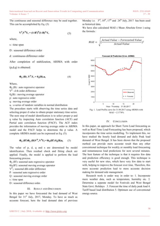
2) It analyzed historical hourly load data from 2017 to build an ARIMA model and forecast demand for July 31, 2017, achieving a Mean Absolute Percentage Error of 2.1778%.
3) ARIMA is identified as an appropriate univariate time series method for short term load forecasting that provides more accurate results than other techniques.
![International Journal on Recent and Innovation Trends in Computing and Communication ISSN: 2321-8169
Volume: 6 Issue: 7 37 - 39
______________________________________________________________________________________
39
IJRITCC | July 2018, Available @ http://www.ijritcc.org
_______________________________________________________________________________________
REFERENCES
[1] Muhammad Usman Fahad and Naeem Arbab, “Factors affecting
short term load forecasting” in Journal of Clean Energy
Technologies, vol.2, no. 4, October 2014
[2] Jonathan Schachter and Pierluigi Mancarella “A Short-term
Load Forecasting Model for Demand Response Applications”.
978- 1- 4799-6095-8/14/$31.00 ©2014 IEEE
[3] Weather Forecast and Report. Available online:
http://www.wunderground.com (accessed on 18 November
2016).
[4] Zhang, P.; Wu, X.; Wang, X.; Bi, S. Short-term load forecasting
based on big data technologies. CSEE . Power Energy Syst.
2015, 1, 59–67.
[5] Yuancheng Li, Panpan Guo and Xiang Li, “Short-Term Load
Forecasting Based on the Analysis of User Electricity
Behavior”.North China Electric Power University, Beijing
102206, China; 23 November 2016
[6] Arjun Baliyan, Kumar Gaurav, “A Review of Short Term Load
Forecasting using Artificial Neural Network Models”, ICCC
2017.](https://image.slidesharecdn.com/9153242930124-07-2018-190130155039/85/Short-Term-Load-Forecasting-Using-ARIMA-Technique-3-320.jpg)