A data-driven model is based on the analysis of the data about a specific system.

1. Data Driven Models and Machine Learning (ML) Approach in Water Resources Systems
Andres M. Ticlavilca1
and Alfonso Torres2
1. Introduction and Overview
1.1 Data-Driven Models
A data-driven model is based on the analysis of the data about a specific system. The main
concept of data-driven model is to find relationships between the system state variables (input and
output) without explicit knowledge of the physical behavior of the system (Solomatine et al.
2008). Examples of data-driven models applied in water resources system and hydrology are the
rating curve, unit hydrograph method, statistical models (that include linear regression,
Autoregressive moving average (ARMA) and Autoregressive integrated moving average
(ARIMA) models) and machine learning (ML) models (Solomatine and Ostfeld 2008).
ML theory is related to pattern recognition and statistical inference wherein a model is capable of
learning to improve its performance of a task on the basis of its own previous experience
(Mjolsness and DeCoste 2001). Examples of ML models include artificial neural networks
(ANNs), support vector machines (SVMs), and relevance vector machines (RVMs).
ML approach is the study of computational methods and algorithms for improving performance
by mechanizing the acquisition of knowledge from experience. ML aims to provide increasing
levels of automation in the knowledge engineering process, replacing much time-consuming
human activity with automatic techniques that improve accuracy or efficiency by discovering and
exploiting regularities in training data. (Simon and Langley 1995). Considering this, ML have
been used for a long time in mathematics, statistics and engineering with models or algorithms
like linear, polynomial regression, time series regression, etc. Some of the tasks learning
machines have been used for are include in Table 1.1.1:
Table 1.1.1 Example of Data-driven models in Water Resources
Task Example of use
Anomaly
detection
Identification of unusual data records (outliers, pattern change, data
deviation) in weather or hydrological time series variables
Association rule
learning
Discovery of relationships (dependency) between variables from different
sources for a given phenomena, e.g. identification of critical weather
variables, vegetation cover and urban development information to explain the
change of lake water levels in time.
Clustering Detection of groups and structures in the data that is alike, without using
known structures or relationship for the data. For example, detection of areas
with similar weather-hydrological patterns is the Western US.
Classification Discovery of structures in the data to identify patterns among them. For
example, identification of vegetation covertures in aerial or satellite image.
Regression Identification of a mathematical expression or equation that models the data
with the least error. E.g. prediction of water flow in rivers based on weather
parameters and local geographic conditions
Summarization Compact representation of data (visualization and report). E.g. Reduction of
LandSat TM/ETM+ satellite bands from 7 to 3 using Principal Component
Analysis.
(1),(2) Postdoctoral Fellow at Utah Water Research Laboratory

2. 1.2 Why ML approach in Water Resource Systems?
Many modeling techniques based on physical principals have been developed to understand the
behavior of hydrologic and water resources systems. In physically based modeling, the input-
output relationship is obtained by the development and solution of fluid mechanics and
thermodynamics equations, with appropriate and detailed boundary conditions, to describe the
dynamics of water throughout the hydrologic system in question. However, solution for
physically based models often require simplifying assumptions, because physiographic and
geomorphic characteristics of most hydrologic systems are complicated, and have a large degree
of uncertainty in the boundary conditions (Brutsaert 2005). Moreover, the practical application of
physically based models can be limited by the lack of required data and the expense of data
acquisition. To overcome these limitations, researchers have used data-driven models based on
ML approach as an alternative to physically based models (Khalil et al. 2005a; Solomatine and
Shrestha 2009). In the ML approach, a model is formulated to link the macro-description of the
behavior of a system (output) to the behavior of the constituents of this system (inputs)
(Guergachi and Boskovic 2008).
Nowadays, many, if not most, of the time series characteristics of hydrology and water resources
systems are nonstationary. Therefore, it is necessary to use methods that can model the
nonstationary behaviors of environmental variables to optimize water systems (Milly et al. 2008).
This implies that using classical statistics, which assume that the time series are stationary (such
as ARMA models), are not suitable. ARIMA models can be used because they take into account
non-stationary behaviors of the time series. However, they use a linear parametric approach,
which can lead to poor performance results when the model is tested with unseen data. Also,
ARIMA models are not suitable if we want to use them for long term forecasting (e.g. streamflow
forecasting up to 12 months ahead) since the long term forecast asymptotically approaches the
mean value of the time series data (Shumway and Stoffer 2011). Studies proved that machine
learning models are more suitable than ARIMA models in learning the nonlinear dynamics and
nonstationary behavior of water resources systems with the final purpose of making accurate
predictions for previously unseen values (Pulido Calvo et al. 2003 and Nourani et al. 2009).-
2. Theoretical Background
2.1 Regression and Classification problem
In general, two major areas where engineering analysis is required are modeling or simulation of
a given occurring phenomena (regression analysis), and identification or categorization of
occurring events or patterns (classification analysis). These two major areas come with their
unique characteristics in terms of objectives to achieve, data sources, and post-calibration
implementation, requiring adequate approaches for a successful model development.
2.1.1 Regression Analysis
The regression analysis includes any technique or algorithm used for mapping or linking several
variables among them. The focus is to develop a relationship among one or several dependent
variables (outputs) with one or more independent variables (inputs). This relationship in ML
algorithms is similar in form to what have been seen for classical data-driven models e.g. linear or
polynomial equations, ARIMA, ARMA, Quantile Regression, to cite some of them. Therefore, a
common property for the regression analysis is that the input-output mapping is expressed in the
form of a mathematical expression. Nevertheless, for more sophisticated ML algorithms, their

3. mathematical representation is quite complex for most of the cases (including initial data
transformation) with the corresponding difficulty to interpret the components of the algorithm
directly. This is one of the reasons why these machines were also called “black box algorithms”.
The regression analysis can involve simulation, forecasting, rule extraction, processes
automation, etc. This analysis can also be used to understand the importance of certain inputs
related to the output variables, and the forms of these relationships.
In regression problems we want to model a continuous dependent variable from a number of
independent variables. For example, a general linear regression problem can be explained by
assuming some dependent or response variable yi (e.g streamflow, evapotranspiration, reservoir
releases, etc) which is influenced by inputs or independent variables xi1, xi2,....,xiq ( e.g. runoff, air
temperature, irrigation water demands, etc). This relation can be expressed by a regression model:
yi= β1 xi1 + β2 xi2 + .....+ βq xiq + ε (2.1.1)
where β1, β2,..., βq are fixed regression parameters and ε is a random error or noise parameter. It is
important to mention that ML approaches are nonlinear regression models in which they use
parametric techniques that assume a functional form that can approximate a large number of
complex functions by using non-linear transformation of a large number of parameters (Ticlavilca
et al. 2011).
2.1.2 Classification Analysis
The classification analysis is related to the categorization or labeling of a given group of variables
values into a pre-defined possible list of groups (in some cases the pre-defined groups is not
necessary or available). The variables in this case are not necessarily defined as input – outputs
groups like in regression analysis. Instead, there are two type of classification analysis, one that
uses predefined categorized groups that allow training the ML algorithms (supervised learning)
and a second type where the algorithm is asked to find certain number of groups or labels that
could be occurring in the data (unsupervised learning).
The identification of a group of variables into a given category or class is usually determined by a
measurement of the closeness of their values to certain clusters centers for each or category/label.
Given that the result from the classification model is integer values or labels, the mathematical
expression for this type of analysis is quite different to what is used in regression.
Classification analysis is often used to determine categories or levels among the occurring data,
changes in the statistical characteristics of incoming data, data failure detection, etc.
2.2 Supervised and Unsupervised Learning
From a theoretical point of view, ML algorithms are divided into two main groups called:
supervised- and unsupervised-learning. The major difference between these groups is the
causality among the variables and the type of results obtained.
For supervised-learning algorithms, there is a relationship of causality predefined by the user or
modeler that is specified before providing the variables to the ML models. For example, most
regression analyses are supervised-learning process. The researcher or user defines which
variables are considered dependent of others (outputs – inputs). Also, some classification tasks

4. are supervised-learning processes given that the causality among the variables is defined by the
user (type and number of groups or labels).
For unsupervised-learning processes, the relationship of causality among the variables is
unknown. Therefore there are not outputs, but only inputs for which the ML algorithm determines
the relationship among them. Classification algorithms like K-Nearest Neighbor and Self
Organizing Feature Maps fall into this category. These algorithms use metrics to define the
closeness of variable values to others and based on these grouping results, define the number of
groups or labels that exist in a given data set. A short example of ML algorithms based on their
learning type is shown is Table 1.2.
Table 2.2.1 Example of use of Data-driven algorithms by type of learning
Data-Driven Algorithm Supervised Learning Unsupervised
Learning
Artificial Neural Networks (ANN) Classification,
Regression,
Association Rule Learning,
Clustering,
Support Vector Machines (SVM) Classification,
Regression,
Association Rule Learning,
Clustering,
Anomaly Detection
Random Forest (RF) Classification,
Regression,
Association Rule Learning
Clustering,
Relevance Vector Machines (RVM) Classification,
Regression,
Association Rule Learning
Classification And Regression Trees (CART) Classification,
Regression,
Clustering,
Linear Discriminant Analysis Classification
2.3 Artificial Neural Networks (ANN)
The Artificial Neural Networks (ANN) is one of the most known ML algorithm inspired by the
architecture of real brains. The fundamental component of this algorithm is the artificial neuron
or nodes that connect and transmit the information altering it according to the data used to
calibrate the neurons as its biological counterpart.
There have been developed a wide range of algorithms based on the ANN notion, differing in
type of architecture, treatment of data (input-output), learning process etc. Nevertheless the main
components for an ANN can be summarized as:
• Network architecture: Number of neurons and layers of neurons for the ANN model.
• Activation function: How a neuron's output depends on its inputs.
• Learning rule: How the strength of the connections between neurons changes over time.

5. In the area of water resources and engineering in general, several ANN types have been tested
and reported, showing their strength or weakness for a specific problem. A representative review
of applications of ANN algorithms in the area of water resources is given by Maier and Dandy
(2000).
2.3.1 Bayesian Multi-Layer Perceptron
The Multi-Layer Perceptron (MLP) is reported to be one of the most widely used models of ANN
(Nabney, 2001). This ANN algorithm is attractive because of its ability to approximate any
smooth function, considering that enough information about the under study phenomena is
available to calibrate the MLP parameters (Bishop, 2007).
Despite of being considered an established technique in the field of hydrology (Londhe and
Charhate, 2010), one of the critical issues often mentioned for ANN algorithms is the absence of
uncertainty measurements associated with the predicted output (Khan and Coulibaly, 2005). To
overcome this limitation, Bishop (2007) implemented the Bayesian Inference framework
(MacKay, 1992) for the calibration of the MLP parameters (BMLP). This had made possible the
additional measurement of the uncertainty related with the predicted outputs. The BMLP
architecture can be described as:
( )
∑ ∑
= =
+
+
⋅
=
H
1
h
(n)
1
h
i
hi
(n)
h
(n)
b
b
x
Wa
tanh
Wb
y
I
i
(2.3.1)
where:
y(n)
: the dependant variables vector (outputs of the model),
xi: ith
component of the independent variables (inputs) vector x(n)
=[x1,… xi…xI],
Wahi, Wbh
(n)
: matrix weights for the first and second layer respectively,
I: number of inputs in the MLP,
H: number of hidden neurons,
b(n)
, bh: bias values for the first and second layer respectively.
Using a dataset D = [x(n)
, t(n)
] with n =1…N, where N is the number of training examples provided
to the BMLP, the training of the parameters [Wa, Wb, b(n)
, bh] is performed by minimizing the
Overall Error Function E (Bishop, 2007):
( ) ∑
∑
W
1
i
2
i
N
1
n
2
(n)
(n)
W
D w
2
α
y
-
t
2
β
E
α
E
*
β
E
=
=
+
=
×
+
=
(2.3.2)
Where:
ED: data error function,
EW: penalization term,
W= number of weights and biases in the neural network, and
α and β: Bayesian hyperparameters.

6. In Bayesian terms, the goal is to estimate the probability of the weights and bias of the MLP
model, given the dataset D:
( ) ( ) ( )
( )
(n)
(n)
(n)
t
p
W
p
W
|
t
p
t
|
W
p
⋅
= (2.3.3)
Where, as explained by MacKay (1992),
p(W|t(n)
): the posterior probability of the weights,
p(t(n)
|W): the likelihood function,
p(W): the prior probability of the weights, and
p(t(n)
): the evidence for the dataset.
For regression tasks, the Bayesian Inference method allows the prediction y(n)
and the variance of
the predictions σy
2
, once the distribution of W has been estimated by maximizing the likelihood
for α and β (Bishop, 2007). σy
2
is the output variance vector σy
2
= (σ1
2
,…, σk
2
,…, σK
2
). This can be
expressed as:
g
H
g
β
σ 1
T
1
2
y
−
−
+
= (2.3.4)
The output variance has two sources; the first source arises from the intrinsic noise in the output
values 1
β−
; and the second source comes from the posterior distribution of the BMLP weights.
The output standard deviation vector σy can be interpreted as the error bar for confidence interval
estimation (Bishop, 2007).
For classification tasks, the Bayesian Inference method allows for the estimation of the likelihood
of belonging to a given class of the input variables. This is an improvement over other
classification-type learning machine algorithms which only provide a single class value (Bishop,
2007).
2.4 Relevance Vector Machine for Regression
Tipping (2001) introduced the Relevance Vector Machine (RVM), a Bayesian approach for
regression models. RVM can be used via its Bayesian approach to avoid overfitting during
parameter estimation, to guaranty generalization performance (robustness). ML theory faces the
issue of how best to update models on the basis of new data and how to seek parsimony in the
model formulation (Mjolsness and DeCoste, 2001). Parsimony is associated with the principal of
Ockham’s razor which can be translated in ML theory as: “a model should be no more complex
than is sufficient to explain the data” (Mjolsness and DeCoste 2001; Tipping 2006). Tipping
(2006) stated that the effect of Ockham’s razor is an automatic and satisfying consequence of
applying the Bayesian framework. In recent years, papers in water resources modeling have
demonstrated that applying the RVM approach can result in a parsimonious model capable of a
robust prediction of water system state. In addition, they have the capability to estimate the
uncertainty of the prediction (Khalil et al. 2005a; Khalil et al. 2005b; Ghosh and Mujumdar
2007). Ticlavilca and McKee 2011, Torres et al. 2011 and Ticlavilca et al. 2011, applied an
extension of the RVM model, The Multivariate Relevance Vector Machine (Thayananthan et al.,
2008) to handle multivariate outputs represented by multiple-time-ahead forecasts applications in
a multiple reservoir system, evapotranspiration and irrigation canal demand respectively.

7. This section summarizes a description of the RVM for regression. Readers interested in greater
detail regarding sparse Bayesian regression, its mathematical formulation and the optimization
procedures of the model are referred to Tipping (2001).
Given a training data set of input-target vector pairs {xn, tn}
N
1
n= , where N is the number of
observations, x Є R D is a D-dimensional input vector, t Є R is a target vector; the model has to
learn the dependency between input and output target with the purpose of making accurate
predictions of t for previously unseen values of x:
t = y + ε
= Φ(x) w+ ε (2.4.1)
where w is a vector of weight parameters and Φ(x) = [1, K(x,x1,… K(x,xN)) is a design matrix
where K(x,xn) is a fixed kernel function. The error ε is conventionally assumed to be zero-mean
Gaussian with variance σ2
.
A Gaussian likelihood distribution for the target vector is written as:
⎪
⎭
⎪
⎬
⎫
⎪
⎩
⎪
⎨
⎧ −
−
= −
−
2
2
N
2
/
N
2
2
y
t
exp
)
2
(
)
,
w
|
t
(
p
σ
σ
π
σ
(2.4.2)
Tipping (2001) proposed imposing an additional prior term to avoid that the estimation of w and
σ2
suffer from severe over-fitting from Eq 2.4.2. This prior is added by applying a Bayesian
perspective, and thereby constraining the selection of parameters. Tipping (2001) defined an
explicit zero-mean Gaussian prior probability distribution over the weights:
⎟
⎟
⎠
⎞
⎜
⎜
⎝
⎛
−
= ∏
=
−
2
w
exp
)
2
(
)
|
w
(
p
2
m
m
M
1
m
2
/
1
m
2
/
M α
α
π
α
(2.4.3)
where M is the number of independent hyperparameters α = (α,..., αM)T
. Each α is associated
independently with every weight (Tipping 2001).
Bayesian inference considers the posterior distribution of the model parameters, which is given
by the combination of the likelihood and prior distributions:
)
,
|
t
(
p
)
|
w
(
p
)
,
w
|
t
(
p
)
,
,
t
|
w
(
p 2
2
2
σ
α
α
σ
σ
α =
(2.4.4)
The main concept in Eq. 2.4.4 is explained by Tipping (2003): “ we have updated our prior
“belief” in the parameter values in light of the information provided by the data t, with more
posterior probability assigned to values which are both probable under the prior and which
“explain the data” “.
The optimal set of hyperparameters αopt and noise parameters (σopt
)2
can be obtained by
maximizing the marginal likelihood (Tipping 2001). During the optimization process, many
elements of α go to infinity, for which the posterior probability of the weight becomes zero. The
few nonzero weights are the relevance vectors (RVs) which generate a sparse representation.

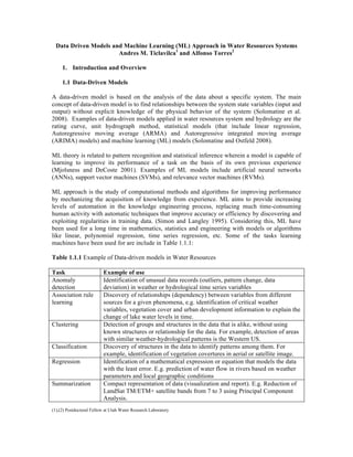
8. As an illustrative example, we explain the "sinc" function with a RVM model (Fig 2.4.1). The
data where the model is trained on based on 100 noisy samples. The estimated function is drawn
as solid blue lines, the true sinc function in red and the RVs are shown as green circles.
Figure 2.4.1. RVM approximations to "sinc" function
2.5 Generalization and Robustness Analysis
Some times ML applications face the problems of overfitting. This means a ML model shows a
good performance when evaluated the model with the same training data set that has been used to
calibrate the model, but this performance is poor when the model is tested with a new test data
set. That is why, it is necessary to develop ML models to guarantee a good generalization.
Several authors in hydrology and water resources modeling research calibrated their ML models
with one training data set and evaluated the performance of their ML models with a different
unseen test data set. It is done in order to avoid overfitting and evaluate the generalization
performance of ML model in unseen data set.
Crossvalidation can be used with non-Bayesian ML algorithms to avoid overfitting. It allows for
the fine tuning of the ML model parameters by dividing the training data into n-folds and
averaging the goodness-of-fit.
ML applications deal with formulation for ill-posed problems while trying to replicate the
expected response of a system based on measurement data. An ill-posed problem means that an
output may have large changes as a consequence of small changes of the inputs. This is why
additional methods to evaluate robustness performance have been applied for machine learning
applications in water resources topics.
Khalil et al. 2005a, Khalil et al. 2005b, Ticlavilca and McKee 2011, Torres et al. 2011 and
Ticlavilca et al. 2011 applied the bootstrap method (Efron and Tibshirani 1998) to evaluate the
robustness performance of their ML model for water resources, irrigation and hydrology systems.

9. The bootstrap data set is created by randomly sampling with replacement from the whole training
data set. This selection process is independently repeated N times to yield N bootstrap training
data sets. For each of the bootstrap training data sets, a model is built and evaluated over the
original test data set. This bootstrap method is used in order to see the variation in test
performance as we vary the training observations.
3. Application of ML in Water Resource Systems
3.1 Real-Time River Basin Network System
ML models have been successfully applied in water resources management research. Ticlavilca
and McKee (2011) applied a multivariate relevance vector machine (MVRVM) in order to
develop multiple-time-ahead predictions of daily releases from multiple reservoirs in Sevier River
Basin in Utah. Their model forecast the water releases of two reservoirs simultaneously having as
inputs past historical data on reservoir releases, diversion into downstream canals, weather, and
streamflows. Their results demonstrated the successful performance and robustness of machine
learning approach for multiple reservoir release forecast.
Ticlavilca et al. (2011) also proposed a MVRVM model for a irrigation water delivery in Sevier
River Basin in Utah. They presented a robust ML approach to forecast the short-term diversion
demands for three irrigation canals. Their model recognized the patterns between multivariate
outputs (future irrigation diversion requirements for three canals) and multivariate inputs (past
data on irrigation diversion demand and climate information). The principal water-delivery
problem in the basin is the inefficient operator responses to short-term changes in demand due to
the lag time between a reservoir flow release and its arrival at the diversion irrigation canals.
Therefore, a model that forecast short term diversion demands can have potential value to assist
the reservoir and canal operators in making efficient real-time operation and management
decisions for available water resources in the basin.
3.2 Evapotranspiration
Torres et al. (2011) aims to produce vital information for water planning for water masters and
managers regarding future reservoir releases. The critical component to accomplish this is future
crop water estimation which is related to adequate evapotranspiration forecast. The model to
develop for ET0 forecasting takes into consideration the following limitations: use of minimum
historical climatic data as usually found at any weather station (in USA and other countries); be
of all-purpose enough to be deployed for any location, and provide updated daily results. Two
Bayesian ML models were tested (BMLP and MVRVM) and nine years of historical daily air
temperature (maximum and minimum) were used. The results indicates that using only historical
temperature data, it is possible to provide a daily ET0 forecast up to 4 days in advance.
3.3 Hydraulic Systems
Automation systems like SCADA – Supervisory Control and Data Adquisition are of common
use in current irrigation systems. These come along with hydraulic simulation systems to allow
water managers and operators to update or change the gates opening and reservoir/canal
discharges based on the real time status of the irrigation system. Nevertheless the use of these
types of technologies in harsh environments like agricultural areas implies that the automation
system is prone to carry along distortions or errors in the measurements along the gates, canals
and other structures that can affect the accuracy of the simulation results. Also these simulation

10. values can be affected by the conceptual approach used to develop the simulation model. This
condition can affect decisions made by the operators and canal controllers about the irrigation
system. As explained in Torres (2011), in order to reduce the impact of the error sources on the
simulation results, a coupled ML – hydraulic simulation model was developed. The used ML
(RVM) defines a relationship among the model stream input (e.g. inflow, water level) with the
aggregate error measured after comparing the simulation results and the actual water level
readings. The results shown by Torres (2011) indicate that the RVM can simulate adequately the
aggregate error values for the simulation model, improving the general simulation results.
4. Illustrative Example
The RVM model for regression is applied to the Sevier Valley/Piute irrigation canal in the Sevier
River Basin, Utah. The data are past daily observations collected by five gauging stations on the
canal (Fig. 4.1) during the 2003-2007 irrigation seasons. Daily data from the 2003 through 2006
irrigation seasons were used to train the RVM model. Daily data from the 2007 irrigation season
were used to test the model.
The outputs are the predictions of canal diversions 1 day ahead from the head gauging station.
The outputs are expressed as :
t = [ Dd]
Two models are compared. The inputs of the first model (Model 1) are past information of the
canal diversions at the head gauging station. The inputs are expressed as:
x= [Dd-nd]
where,
d day of prediction
nd number of days previous to the prediction time
Dd-nd canal diversion "nd" days previous to the prediction time.
The inputs of the second model (Model 2) are past information of the canal diversions and also
information at four gauging stations along the canal: Willow Creek, Aurora, Clairon and End
stations (Fig 4.1). The inputs are expressed as:
x= [Wd-nd Ad-nd Cd-nd Ed-nd Dd-nd]
where,
d day of prediction
nd number of days previous to the prediction time.
Dd-nd canal diversion at Head station "nd" days previous to the prediction time.
Wd-nd canal flow at Willow Creek station "nd" days previous to the prediction time.
Ad-nd canal flow at Aurora station "nd" days previous to the prediction time.
Cd-nd canal flow at Clarion station "nd" days previous to the prediction time.
Ed-nd canal flow at End station "nd" days previous to the prediction time.

11. Fig 4.1. Location of gauging stations on the Sevier Valley/Piute irrigation canal
The statistic used for model selection is the coefficient of efficiency (E) calculated for the testing
phase. It has been recommended by the ASCE (1993) and Legates and McCabe (1999), and is
given by:
∑
∑
=
=
−
= N
1
n
2
av
n
N
1
n
2
n
n
)
t
(t
*)
t
-
(t
-
1
E
where t is the observed output; t* is the predicted output ; tav is the observed average output and
N is the number of observations. This statistic ranges from minus infinity (poor model) to 1.0 (a
perfect model) (Legates and McCabe 1999).
In equation 2.4.1 the basis function (Ф) is defined in terms of a fixed kernel function. It is
necessary to choose the type of kernel function and to determine the value of the kernel width
(Tipping 2001, Ticlavilca and McKee 2010). In this example, we consider a Gaussian kernel
since it has been used in several water resources and hydrology applications.
For both models, several RVM models were built with variation in kernel width and number of
previous time steps. The number of previous time steps was chosen from a range of 1-7 days
previous to the prediction time. The kernel width was chosen from a range of 1-5. The selected
kernel width is the one with maximum E. From the list of models with selected kernel width at
different "nd" values, we considered that the selected model is the one with the maximum E.

12. Table 4.1 Model comparison, test phase
RVM models E RMSE (cfs) nd kernel width # RVs
Model 1 0.989 9.04 6 1 37
Model 2 0.997 4.69 6 1 294
From Table 4.1 we can see that the statistics results of Model 2 shows better performance (higher
E and lower RMSE) than the statistics of Model 1. Also, we can see that both models need 6
previous days as inputs.
The relevance vectors (RVs) are subsets of the training data that are part of the model structure
after finding the optimized parameters. The complexity of the model is proportional to the
number of RVs. Model 1 and Model 2 only utilize 37 and 294 RVs respectively from the training
data set (1035 observations) that was used for training ( 2003 through 2006 irrigation seasons).
We can see that Model 1 is sparser than Model 1. It is because Model 1 use data from one station
as inputs while Model 2 use data from five stations that represent the whole irrigation canal
system. The main point here is to show that RVM is capable of producing sparse models. The
percentage of relevance vectors (RVs) that where used to build Model 1 and Model 2 from the
training data set are respectively 4 and 28 %. This means that the model ignores a high percentage
of observations to avoid over-fitting. This low percentage illustrates that the Bayesian learning
procedure embodied in the RVM is capable of producing sparse models. Therefore, we can see an
important advantage of using RVM models which are capable of reducing model complexity to
avoid over-fitting.
Fig 4.2. Model 1, Predicted vs. Observed with 0.90 confidence intervals (shaded region), Sevier
Valley/Piute canal diversions, Test phase from July to September 2007

13. Fig 4.3. Model 2, Predicted vs. Observed with 0.90 confidence intervals, Sevier Valley/Piute
canal diversions, Test phase from July to September 2007
Due to its Bayesian approach, the output result of the RVM is the mean of a predictive
distribution of each output. Then, the predictive confidence intervals for each output can be
determined. This predictive interval (which is based on probabilistic approach) should not be
confused with a classical frequentist confidence interval (which is based on the data).
We plotted the test results (observed vs. predicted) from July to September 2007 for both models
(Figs. 4.2 and 4.3). We can see that for Model 1 (Fig. 4.2) the predictive confidence intervals
(shaded region) are wider than the ones from Model 2 (Fig. 4.3). Also, Model 1 shows a lag of
about one day between the observed (dots) and predicted (line). This lag issue is not observed in
Model 2, and it is because the model performs much better when we added more inputs data that
directly represent the irrigation canal system and let the RVM learns the patterns.
The bootstrap method is applied to Model 2 to guarantee robustness of the RVM model. It is
created by randomly sampling with replacement from the whole training data set. This process
was independently repeated 1000 times to yield 1000 bootstrap training data sets. For each of the
bootstrap training data sets, a model was built and evaluated over the test data set (2007 irrigation
season).

14. Fig 4.4. Bootstrap histogram of the RVM Model 2 for the E test.
The bootstrap method provides implicit information on the uncertainty in the statistics estimator
evaluated in the RVM model (in this case the coefficient of efficiency E). A robust model is one
that shows a narrow confidence bounds in the bootstrap histogram (Khalil et al. 2005b) such as
this illustrated in Fig 4.4.
In this section, we have presented an example of a RVM model for daily canal diversion
forecasting. The results have demonstrated the successfully RVM performance in terms of
accuracy and robustness.
5. Discussions
While in the previous sections data-driven tool characteristics and uses where shown; in this
section it is discussed the restrictions for using these techniques.
• A critical factor for the use of ML models is data availability. Data-driven tools calibration
process is based on patterns that the algorithm can “learn” from the data. Amount of data
should be enough to divide in training and testing subsets. In the case of time series or
historical data, it is recommendable to have at least three complete cycles of the
phenomena(s) under analysis (e.g. irrigation seasons or runoff years) and its or their
respective inputs or cases. Two cycles would be separated for training and the most recent
cycle for testing the ML model accuracy.

15. • There are two aspects to considerate when calibrate a ML model. One is the input calibration
of the data-driven tool. Each ML model has its unique parameters. For example ANN models
require the selection of the number of hidden neurons and the learning function. RVM models
require the selection of the type of kernel and a kernel width value. The second aspect is the
selection of the most adequate inputs for a parsimonious model. There is not a unique
methodology for both of these aspects being tied to the characteristics of the learning
machine. For example a BMLP model can identify 5 out 10 variables to provide an excellent
approximation for a discharge forecast, while a RVM model can select 4 variables. These
variables are not necessarily the same as the ones for the BMLP, but both data-driven
algorithms achieve similar performance. This is related to the type of synergy or interaction
among variables that each algorithm is able to identify. There are some general techniques
that can facilitate the selection of the adequate inputs as explained by Guyon & Elisseeff
(2003): forward and backward variable selection, automatic relevance determination (for
Bayesian-based algorithms) or combination of these techniques.
• How to determine the accuracy of the calibrated ML model is another important point. The
selection of the relevance goodness-of-fit parameters is important. For regression problems
the coefficient of efficiency has been used extensively in research along with the Root Mean
Square Error (RMSE). Also the error bar (also called noise) for Bayesian learning machines
is an indicative of the summed error in the data and algorithm. For classification-type
problems the Error Class Matrix is indispensable along the Kappa Index, which measures the
accuracy of the model predicting the different classes vs. the probability of random
occurrence.
• For time series models a couple of important issues occur along the time dimension. First,
sometimes a time lag between the simulated and the true signal occurs. In most cases this is
an indication of missing inputs into the model. Second, the characteristics of the residuals or
the difference between the simulated and the true signal. The residuals should comply with
random or white noise characteristics (normal, independent, identically distributed). The
absence of these characteristics indicates that some pattern in the data is not fully captured by
the ML model because of one or several reasons: inadequate ML model calibration, limited
amount of historical data, missing inputs, etc). These issues are not evident by the fit statistics
requiring additional tests (statistical or graphical) to be applied.
• Finally, validation of the quality of data and its sources is a critical step for the application of
ML models. While some extreme cases or outliers in the training data might get ignored by
the data-driven algorithm, the quality of the information should be verified by the user before
its use. Therefore QA/QC (quality assurance and control) techniques are of importance for
data validation.
6. Conclusions
This chapter was intended to share the authors’ experience in the use and application of statistical
data driven algorithms for water resources issues. The final conclusions that can be drawn are:
• ML models or data-driven techniques are additional tools for use in water resources
engineering that can complement, improve (or replace in some scenarios) physical-based
models. The main advantage of these tools is their capability to capture complex nonlinear
patterns and trends in the available data.
• While physical-based models (e.g. rainfall-runoff) components allows for the analysis of their
internal components, the imbedded components of data-driven tools do not allow for a direct
interpretation yet (black-box algorithms).

16. • ML models in most cases have a better performance than physical-based model; nevertheless
they are limited by the quality and availability of information.
• The use of ML models is recommended under the following scenarios: incomplete data to
develop physical-based models, extensive records of the phenomena and related causes or
inputs, data forecasting, and classification-type problems.
7. References
ASCE Task Committee on Definition of Criteria for Evaluation of Watershed Models of the
Watershed Management, Irrigation, and Drainage Division (ASCE) (1993) Criteria for
evaluation of watershed models. J Irr Drain Eng 119(3):429-442.
Bishop, C. (2007). Neural networks for pattern recognition (1st ed.). Oxford: Oxford University
Press. Retrieved from http://www.worldcat.org/title/neural-networks-for-pattern-
recognition/oclc/629691902
Brutsaert W (2005) Hydrology, an introduction. Cambridge University Press, NY.
Efron, B., & Tibshirani, R. J. (1993). An Introduction to the Bootstrap. (C. HallCRC,
Ed.)Chapman and Hall (Vol. 57, p. 436). Chapman & Hall. Retrieved from
http://books.google.com/books?id=gLlpIUxRntoC&pgis=1
Ghosh S, Mujumdar PP (2007) Statistical downscaling of GCM simulations to streamflow using
relevance vector machine, Adv Water Resour 31:132-146.
Guergachi A, Boskovic G (2008) System models or learning machines? Appl Math Comp
204:553–567.
Guyon, I., & Elisseeff, A. (2003). An introduction to variable and feature selection. (L. P.
Kaelbling, Ed.)The Journal of Machine Learning Research, 3(7-8), 1157–1182. JMLR. org.
doi:10.1162/153244303322753616
Khalil A, Almasari M, McKee M, Kemblowski MW, Kaluarachchi J (2005a) Applicability of
statistical learning algorithms in groundwater quality modeling. Water Resour Res
41:W05010.
Khalil A, McKee M, Kemblowski MW, Asefa T (2005b) Sparse Bayesian learning machine for
real-time management of reservoir releases. Water Resour Res 41:W11401.
Khalil A, McKee M, Kemblowski MW, Asefa T, Bastidas L (2005c) Multiobjective analysis of
chaotic dynamic systems with sparse learning machines. Advances in Water Resources 29:
72-88.
Khalil A, McKee M, Kemblowski MW, Asefa T (2005d) Basin-scale water management and
forecasting using neural networks. J Am Water Resour Res 41:195-208.

17. Khan, M. S., & Coulibaly, P. (2005). Streamflow forecasting with uncertainty estimate using
Bayesian learning for ANN. Proceedings. 2005 IEEE International Joint Conference on
Neural Networks, 2005. (Vol. 5, pp. 2680-2685). IEEE. doi:10.1109/IJCNN.2005.1556347
Langley, P., & Simon, H. A. (1995). Applications of machine learning and rule induction.
Communications of the ACM, 38(11), 54–64. ACM. doi:10.1145/219717.219768
Legates D R, and McCabe G J (1999) Evaluating the use of “goodness-of-fit” measures in
hydrologic and hydroclimatic model validation. Water Resour Res 35(1):233-241.
Londhe, S., & Charhate, S. (2010). Comparison of data-driven modelling techniques for river
flow forecasting. Hydrological Sciences Journal, 55(7), 1163-1174.
doi:10.1080/02626667.2010.512867
MacKay, D. J. C. (1992). A Practical Bayesian Framework for Backpropagation Networks.
Neural Computation, 4(3), 448-472. doi:10.1162/neco.1992.4.3.448
Maier, H. R., & Dandy, G. C. (2000). Neural networks for the prediction and forecasting of water
resources variables: a review of modelling issues and applications. Environmental
Modelling & Software, 15(1), 101-124. doi:10.1016/S1364-8152(99)00007-9
Milly, P C D, Julio Betancourt, Malin Falkenmark, Robert M Hirsch, Zbigniew W Kundzewicz,
Dennis P Lettenmaier, and Ronald J Stouffer. 2008. Climate change - Stationarity is dead:
Whither water management? Science 319, no. 5863: 573-574.
Mjolsness E, DeCoste D (2001) Machine learning for science: state of the art and future
prospects. Science 293:2051–2055.
Nabney, I. T. (2001). NETLAB: algorithms for pattern recognition. Springer. Retrieved from
http://www.ncrg.aston.ac.uk/netlab/book.html
Nourani V, Mehdi K, Akira M (2009) A multivariate ANN-wavelet approach for rainfall–runoff
modeling. Water Resour Manage 23:2877–2894
Pulido-Calvo I, Roldan J, Lopez-Luque R, and Gutierrez-Estrada J C. Demand forecasting for
irrigation water distribution systems (2003). Irr Drain Eng 129(6):422-431.
Simon, H. A. H. A., & Langley, P. (1995). Applications of machine learning and rule induction.
Communications of the ACM, 38(11), 54-64. ACM. doi:10.1145/219717.219768
Shumway RH and Stoffer DS (2011) Time series analysis and its applications. Third edition.
Springer. USA.
Solomatine DP, Shrestha DL (2009) A novel method to estimate model uncertainty using
machine learning techniques, Water Resour Res 45:W00B11.
Solomatine, DP, and Ostfeld (2008), A. Data-driven modelling: some past experiences and new
approaches. J of Hydroinformatics,10(1), 3-22.

18. Solomatine, DP, Abrahart, R., See L. (2008). Data-driven modelling: concept, approaches,
experiences. , In: Practical Hydroinformatics: Computational Intelligence and
Technological Developments in Water Applications (Abrahart, See, Solomatine, eds),
Springer-Verlag.
Thayananthan A, Navaratnam R, Stenger B, Torr PHS, Cipolla R (2008) Pose estimation and
tracking using multivariate regression. Pattern Recognit Lett 29(9):1302-1310.
Tipping ME (2001) Sparse Bayesian learning and the relevance vector machine. J Mach Learn
1:211–244.
Ticlavilca AM and McKee M (2011) Multivariate Bayesian regression approach to forecast
releases from a system of multiple reservoirs. Water Resour Manage 25:523–543
Ticlavilca, A. M., M. McKee, and W. R. Walker. 2011. Real-time forecasting of short-term
irrigation canal demands using a robust multivariate Bayesian learning model. Irrigation
Science”. DOI 10.1007/s00271-011-0300-6
Tipping ME (2001) Sparse Bayesian learning and the relevance vector machine. J Mach Learn
1:211–244.
Tipping M (2006) Bayesian inference: an introduction to principles and practice in machine
learning. Adv Lect Mach Learn 41-62.
Tipping M, Faul A (2003) Fast marginal likelihood maximization for sparse Bayesian models,
paper presented at Ninth International Workshop on Artificial Intelligence and Statistics,
Soc. for Artif Intel Stat, Key West, FL.
Torres AF, Walker WR, McKee M (2011) Forecasting daily potential evapotranspiration using
machine learning and limited climatic data, Agricultural Water Management, Volume 98,
Issue 4, Pages 553-562, ISSN 0378-3774, DOI 10.1016/j.agwat.2010.10.012.
Torres AF (2011) Bayesian Data-Driven Models for Irrigation Water Management, Ph.D Thesis,
Civil and Environmental Engineering, Utah State University, Utah.
Valpola, H. (2000). Bayesian ensemble learning for nonlinear factor analysis. Acta Polyt. Scand.
Ma. Helsinki University of Technology.