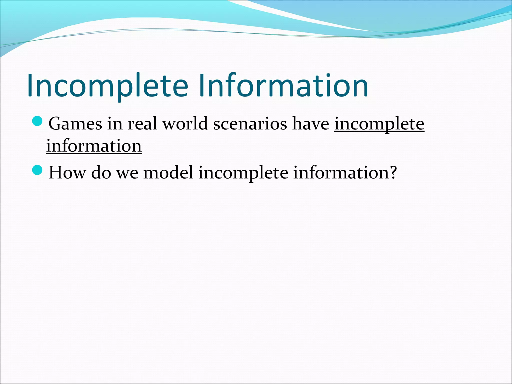
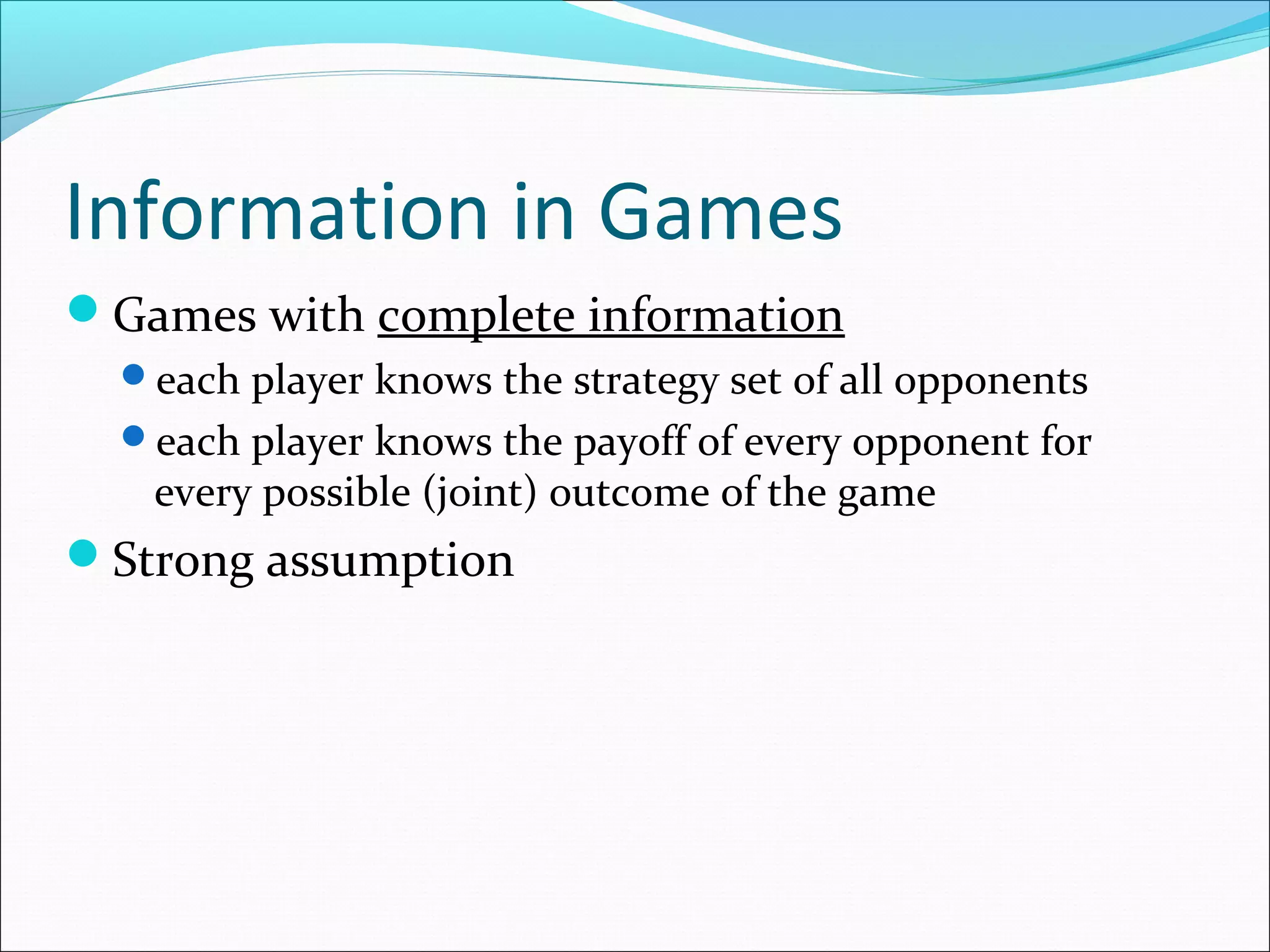
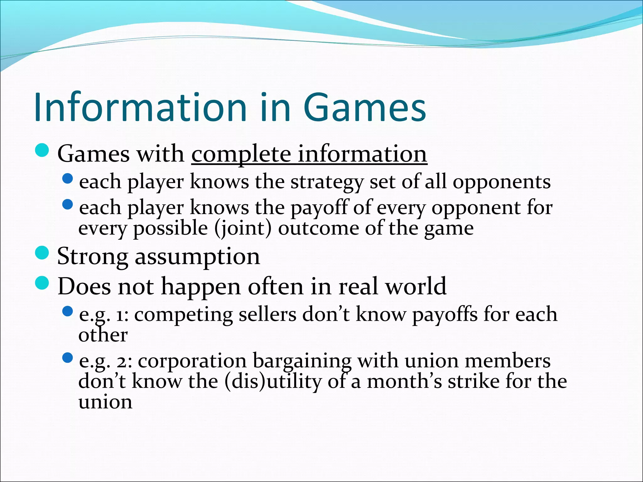
The document discusses games with incomplete information and how they are modeled. It notes: - Games in the real world often have incomplete information where players do not know each other's payoffs or strategies. - Harsanyi's approach models incomplete information using random variables for each player's preferences that are privately observed but have a commonly known probability distribution. This transforms incomplete information into imperfect information. - A Bayesian game formally represents this setting, where a player's utility depends on their type drawn from a probability distribution. A Bayesian Nash equilibrium requires optimal strategies given beliefs over other players' types.

2. Information in Games
Games with complete information
each player knows the strategy set of all opponents
each player knows the payoff of every opponent for
every possible (joint) outcome of the game
Strong assumption

3. Information in Games
Games with complete information
each player knows the strategy set of all opponents
each player knows the payoff of every opponent for
every possible (joint) outcome of the game
Strong assumption
Does not happen often in real world
e.g. 1: competing sellers don’t know payoffs for each
other
e.g. 2: corporation bargaining with union members
don’t know the (dis)utility of a month’s strike for the
union

4. Incomplete Information
Games in real world scenarios have incomplete
information
How do we model incomplete information?

5. Incomplete Information
Games in real world scenarios have incomplete
information
How do we model incomplete information?
Consider a player’s beliefs about other players’
preferences, his beliefs about their beliefs about his
preferences, …

6. Modeling Games with
Incomplete Information
Harsanyi’s approach:
Each player’s preferences are determined by a random
variable
The exact value of the random variable is observed by
the player alone
But…

7. Modeling Games with
Incomplete Information
Harsanyi’s approach:
Each player’s preferences are determined by a random
variable
The exact value of the random variable is observed by
the player alone
But…the prior probability distribution of the random
variable is common knowledge among all players

8. Modeling Games with
Incomplete Information
Incomplete information now becomes imperfect
information
Who determines the value of the random variable for
each player?

9. Modeling Games with
Incomplete Information
Incomplete information now becomes imperfect
information
Who determines the value of the random variable for
each player?
Nature
 background/culture/external effects on each player

10. Example: Modified DA’s
Brother
Prisoner 2 now can behave in one of two ways
with probability µ he behaves as he did in the original
game
with probability 1-µ he gets “emotional”, i.e., he gets an
additional payoff of –6 if he confesses (rats on his
accomplice)
Who determines µ?
“nature” of player 2
Note: Player 1 still behaves as he did in the
original game

11. Type I (prob µ) Type II (prob 1-µ)

12. Example: Modified DA’s
Brother
Player 2 has 4 pure strategies now
confess if type I, confess if type II
confess if type I, don’t confess if type II
don’t confess if type I, confess if type II
don’t confess if type I, don’t confess if type II
Player’s strategy is now a function of its type
Note:
Player 2’s type is not visible to player 1,
Player 1 still has two pure strategies as before

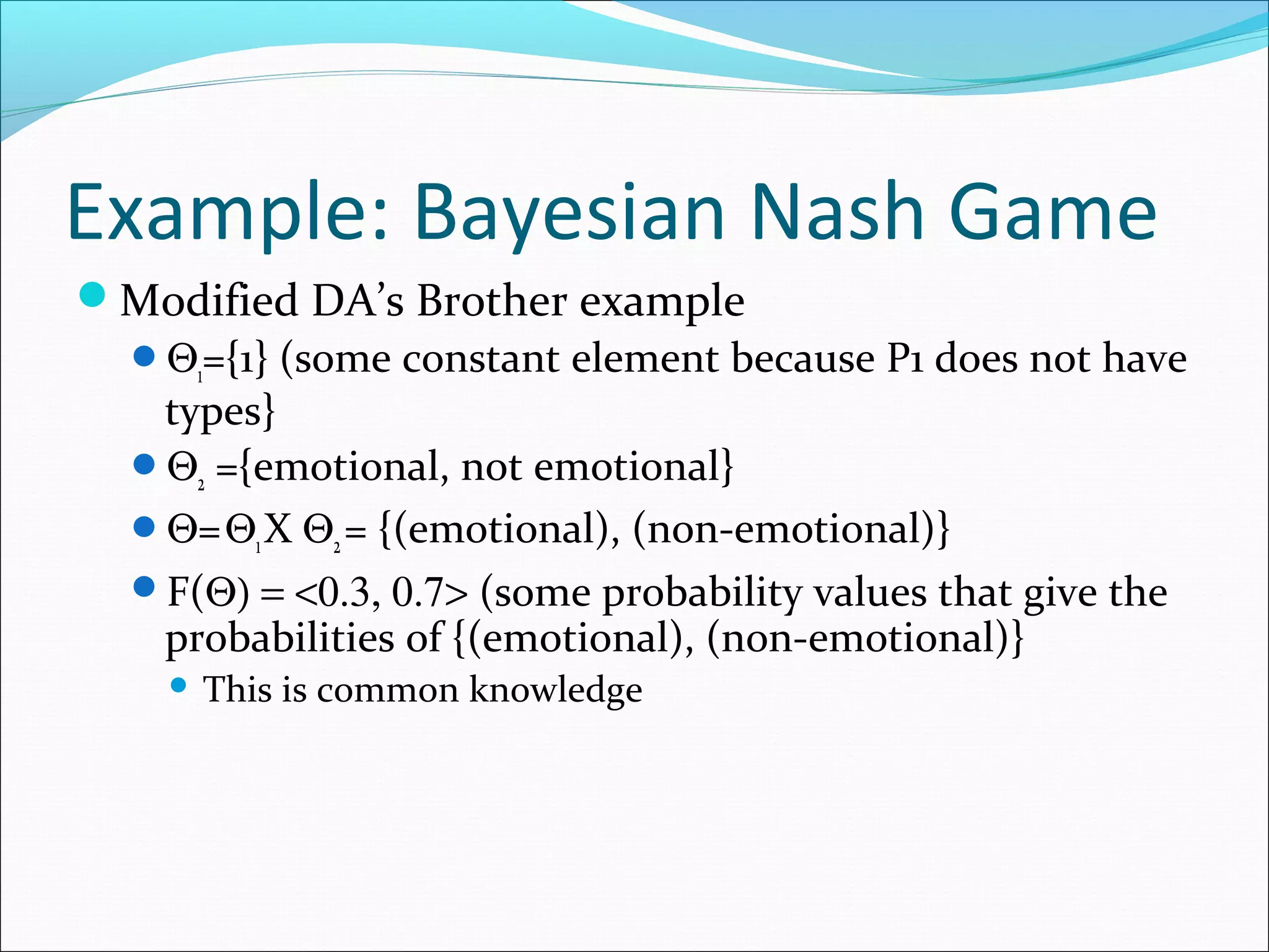
13. Bayesian Nash Game
Player i’s utility is written as:
ui(si,s-i, θi), where θi Є Θi
 θi: random variable chosen by nature
 Θi: distribution from which the random variable
is chosen
F(θ1,θ2,θ3,… θI): joint probability distribution of all
players
common knowledge among all players
 Θ = Θ1 X Θ2 X Θ3 …X ΘI
Bayesian Nash Game = [I, {Si}, {ui(.
)}, Θ, F(.
)]

14. Example: Bayesian Nash Game
Modified DA’s Brother example
Θ1={1} (some constant element because P1 does not have
types}
Θ2 ={emotional, not emotional}
Θ=Θ1X Θ2= {(emotional), (non-emotional)}
F(Θ) = <0.3, 0.7> (some probability values that give the
probabilities of {(emotional), (non-emotional)}
 This is common knowledge

15. Bayesian Nash Game
Pure strategy of a player is now a function of the type
of the player:
si(θi): called decision rule
Player i’s pure strategy set is S iwhich is the set of all
possible si(θi)-s
Player i’s expected payoff is given by:
ûi(s1(.
), s2(.
), s3(.
), ….sI(.
))=Eθ[ui(s1(θ1)...sI(θI), θi)]

16. Bayesian Nash Game as
Normal Form Game
We can rewrite the Bayesian Nash game
[I, {Si}, {ui(.
)}, Θ, F(.
)]

17. Bayesian Nash Game as
Normal Form Game
We can rewrite the Bayesian Nash game
[I, {Si}, {ui(.
)}, Θ, F(.
)]
as
[I, {S i}, ûi(.
)}]

18. Definition: Bayesian Nash Equilibrium
A pure strategy Bayesian Nash equilibrium for the
Bayesian Nash game [I, {Si}, {ui(.
)}, Θ, F(.
)] is a
profile of decision rules (s1(.
), s2(.
), s3(.
), ….sI(.
)) that
constitutes a Nash equilibrium of game [I, {S i},
{ûi(.
)}]. That is, for every i=1…I
ûi(si(.
), s-i(.
)) >= ûi(s’i(.
), s-i(.
))
for all s’i(.
) Є S i where ûi(si(.
), s-i(.
)) is the expected
payoff for player i

19. Proposition
A profile of decision rules (s1(.
), s2(.
), s3(.
), ….sI(.
)) is a
Bayesian Nash equilibrium in a Bayesian Nash
game [I, {Si}, {ui(.
)}, Θ, F(.
)] if and only if, for all i
and all θ’i Є Θi occurring with positive probability
Eθ-i[ui(si(θ’i), s-i(θ-i), θ’i) | θ’i)] >=
Eθ-i[ui(si’, s-i(θ-i), θ’i) | θ’i)]
for all si’ Є Si, where the expectation is taken over
realizations of the other players’ random variables
conditional on player i’s realization of signal θ’i.

20. Outline of Proof (by contradiction)
Necessity: Suppose the inequality (on last
slide) did not hold, i.e.,
Eθ-i[ui(si(θ’i), s-i(θ-i), θ’i) | θ’i)] <
Eθ-i[ui(si’, s-i(θ-i), θ’i) | θ’i)]
→ Some player I for whom θ’i Є Θihappens with a
positive probability, is better off by changing its
strategy and using si’ instead of si(θ’i)
→ (s1(.
), s2(.
), s3(.
), ….sI(.
)) is not a Bayesian Nash equilibrium
→ Contradiction

21. Outline of Proof (by contradiction)
Reverse direction:
Eθ-i[ui(si(θ’i), s-i(θ-i), θ’i) | θ’i)] >=
Eθ-i[ui(si’, s-i(θ-i), θ’i) | θ’i)] holds for
all θ’i Є Θioccurring with positive probability
→ player i cannot improve on the payoff received by
playing strategy si(.
)
→ si(.
) constitutes a Nash equilibrium

22. Type I (prob µ) Type II (prob 1-µ)

23. Solution to Modified DA’s Brother
Prisoner 2, type I plays C with probability 1 (dominant
strategy)
Prisoner 2, type II plays DC with probability 1(dominant
strategy)
Expected payoff to P1 with strategy DC: -10µ +0(1-µ)
Expected payoff to P1 with strategy C: -5µ -1(1-µ)
Player 1:
Play DC when -10µ +0(1-µ) > -5µ -1(1-µ)
or, µ<1/6
Play C when µ>1/6
 µ=1/6 makes player 1 indifferent

24. Weakly Dominated Strategy
Problem of weakly dominated strategy:
for some strategy of the opponent the weakly dominant
and the weakly dominated strategy give exactly same
payoff
player CAN play weakly dominated strategy for some
strategy of the opponent

25. U
D
(D,R) is a Nash equilibrium involving a play
of weakly dominated strategies

26. Perturbed Game
Start with normal form game
ΓN=[I, {∆(Si)}, {ui(.
)}]
Define a perturbed game
Γε= [I, {∆ε(Si)}, {ui(.
)}]
where ∆ε (Sj)={(σi: σi> εi(si) for all si Є Siand Σ siЄ Siσi (si)=1}
 εi(si) denotes the minimum probability of player I playing
strategy si

27. Perturbed Game
Start with normal form game
ΓN=[I, {∆(Si)}, {ui(.
)}]
Define a perturbed game
Γε= [I, {∆ε(Si)}, {ui(.
)}]
where ∆ε (Sj)={(σi: σi> εi(si) for all si Є Siand Σ siЄ Siσi (si)=1}
 εi(si) denotes the minimum probability of player I playing
strategy si
εi(si) denotes the unavoidable probability of playing
strategy siby mistake

28. Definition: Nash equilibrium in
Trembling Hand Perfect Game
A Nash equilibrium of a game ΓN=[I, {∆(Si)}, {ui(.
)}] is
(normal form) trembling hand perfect if there is
some sequence of perturbed games {Γεk }k=1
∞
that
converges to ΓN [in the sense that lim k ∞→ (εi
k
(si) )=0 for
all I and si Є Si] for which there is some
associated sequence of Nash equilibria {σk
} k=1
∞
that
converges to σ (i.e. such that lim k ∞→ σk
= σ)

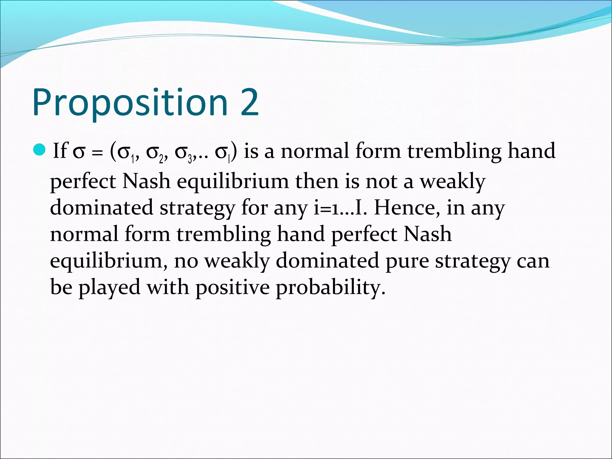
29. Proposition 1
A Nash equilibrium of a game ΓN=[I, {∆(Si)}, {ui(.
)}] is
(normal form) trembling hand perfect if and only if
there is some sequence of totally mixed strategies
{σk
} k=1
∞
such that lim k ∞→ σk
= σ and σi is a best response
to every element of sequence {σk
-i} k=1
∞
for all i=1…I.

30. Proposition 2
If σ = (σ1, σ2, σ3,.. σI) is a normal form trembling hand
perfect Nash equilibrium then is not a weakly
dominated strategy for any i=1…I. Hence, in any
normal form trembling hand perfect Nash
equilibrium, no weakly dominated pure strategy can
be played with positive probability.