2
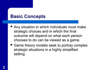
Basic Concepts
Anysituation in which individuals must make
strategic choices and in which the final
outcome will depend on what each person
chooses to do can be viewed as a game.
Game theory models seek to portray complex
strategic situations in a highly simplified
setting.
3.
3
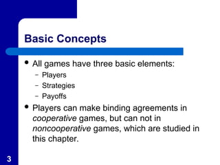
Basic Concepts
Allgames have three basic elements:
– Players
– Strategies
– Payoffs
Players can make binding agreements in
cooperative games, but can not in
noncooperative games, which are studied in
this chapter.
4.
4
Players
A playeris a decision maker and can be
anything from individuals to entire nations.
Players have the ability to choose among a
set of possible actions.
Games are often characterized by the fixed
number of players.
Generally, the specific identity of a play is not
important to the game.
5.
5
Strategies
A strategyis a course of action available to a
player.
Strategies may be simple or complex.
In noncooperative games each player is
uncertain about what the other will do since
players can not reach agreements among
themselves.
6.
6
Payoffs
Payoffs arethe final returns to the players at
the conclusion of the game.
Payoffs are usually measure in utility although
sometimes measure monetarily.
In general, players are able to rank the payoffs
from most preferred to least preferred.
Players seek the highest payoff available.
7.
7
Equilibrium Concepts
Inthe theory of markets an equilibrium
occurred when all parties to the market had no
incentive to change his or her behavior.
When strategies are chosen, an equilibrium
would also provide no incentives for the
players to alter their behavior further.
The most frequently used equilibrium concept
is a Nash equilibrium.
8.
8
Nash Equilibrium
ANash equilibrium is a pair of strategies
(a*,b*) in a two-player game such that a* is an
optimal strategy for A against b* and b* is an
optimal strategy for B against A*.
– Players can not benefit from knowing the equilibrium
strategy of their opponents.
Not every game has a Nash equilibrium, and
some games may have several.
9.
9
An Illustrative AdvertisingGame
Two firms (A and B) must decide how much to
spend on advertising
Each firm may adopt either a higher (H) budget
or a low (L) budget.
The game is shown in extensive (tree) form in
Figure 12.1
10.
10
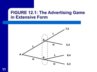
An Illustrative AdvertisingGame
A makes the first move by choosing either H or
L at the first decision “node.”
Next, B chooses either H or L, but the large
oval surrounding B’s two decision nodes
indicates that B does not know what choice A
made.
12
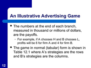
An Illustrative AdvertisingGame
The numbers at the end of each branch,
measured in thousand or millions of dollars,
are the payoffs.
– For example, if A chooses H and B chooses L,
profits will be 6 for firm A and 4 for firm B.
The game in normal (tabular) form is shown in
Table 12.1 where A’s strategies are the rows
and B’s strategies are the columns.
13.
13
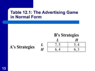
Table 12.1: TheAdvertising Game
in Normal Form
B’s Strategies
L H
L 7, 5 5, 4
A’s Strategies H 6, 4 6, 3
14.
14
Dominant Strategies andNash
Equilibria
A dominant strategy is optimal regardless of
the strategy adopted by an opponent.
– As shown in Table 12.1 or Figure 12.1, the
dominant strategy for B is L since this yields a
larger payoff regardless of A’s choice.
If A chooses H, B’s choice of L yields 5, one better than if
the choice of H was made.
If A chooses L, B’s choice of L yields 4 which is also one
better than the choice of H.
15.
15
Dominant Strategies andNash
Equilibria
A will recognize that B has a dominant strategy
and choose the strategy which will yield the
highest payoff, given B’s choice of L.
– A will also choose L since the payoff of 7 is one
better than the payoff from choosing H.
The strategy choice will be (A: L, B: L) with
payoffs of 7 to A and 5 to B.
16.
16
Dominant Strategies andNash
Equilibria
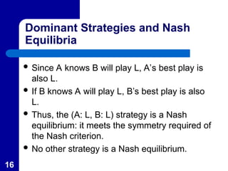
Since A knows B will play L, A’s best play is
also L.
If B knows A will play L, B’s best play is also
L.
Thus, the (A: L, B: L) strategy is a Nash
equilibrium: it meets the symmetry required of
the Nash criterion.
No other strategy is a Nash equilibrium.
17.
17
Two Simple Games
Table 12.2 (a) illustrates the children’s finger
game, “Rock, Scissors, Paper.”
– The zero payoffs along the diagonal show that if
players adopt the same strategy, no payments are
made.
– In other cases, the payoffs indicate a $1 payment
from the loser to winner under the usual hierarchy
(Rock breaks Scissors, Scissors cut Paper, Paper
covers Rock).
18.
18
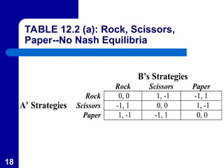
TABLE 12.2 (a):Rock, Scissors,
Paper--No Nash Equilibria
B’s Strategies
Rock Scissors Paper
Rock 0, 0 1, -1 -1, 1
Scissors -1, 1 0, 0 1, -1
A’ Strategies
Paper 1, -1 -1, 1 0, 0
19.
19
Two Simple Games
This game has no equilibrium.
Any strategy pair is unstable since it offers at
least one of the players an incentive to adopt
another strategy.
– For example, (A: Scissors, B: Scissors) provides
and incentive for either A or B to choose Rock.
– Also, (A: Paper, B: Rock) encourages B to choose
Scissors.
20.
20
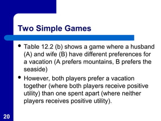
Two Simple Games
Table 12.2 (b) shows a game where a husband
(A) and wife (B) have different preferences for
a vacation (A prefers mountains, B prefers the
seaside)
However, both players prefer a vacation
together (where both players receive positive
utility) than one spent apart (where neither
players receives positive utility).
21.
21
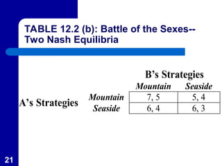
TABLE 12.2 (b):Battle of the Sexes--
Two Nash Equilibria
B’s Strategies
Mountain Seaside
Mountain 7, 5 5, 4
A’s Strategies Seaside 6, 4 6, 3
22.
22
Two Simple Games
At the strategy (A: Mountain, B: Mountain),
neither player can gain by knowing the other’s
strategy.
The same is true with the strategy (A: Seaside,
B: Seaside).
Thus, this game has two Nash equilibria.
23.
23
APPLICATION 12.1: Nash
Equilibriumon the Beach
Applications of the Nash equilibrium concept
have been used to analyze where firms choose
to operate.
The concept can be used to analyze where
firm’s locate geographically.
The concept can also be used to analyze
where firm’s locate in the spectrum of specific
types of products.
24.
24
APPLICATION 12.1: Nash
Equilibriumon the Beach
Hotelling’s Beach
– Hotelling looked at the pricing of ice cream sellers
along a linear beach.
– If people are evenly spread over the length of the
beach, he showed that each seller had an
advantage selling to nearby consumers who incur
lower (walking) costs.
– The Nash equilibrium concept can be used to show
the optimal location for each seller.
25.
25
APPLICATION 12.1: Nash
Equilibriumon the Beach
Milk Marketing in Japan
– In southern Japan, four local marketing boards
regulate the sale of milk.
– It appears that each must take into account what the
other boards are doing, since milk can be shipped
between regions.
– A Nash equilibrium similar to the Cournot model
found prices about 30 percent above competitive
levels.
26.
26
APPLICATION 12.1: Nash
Equilibriumon the Beach
Television Scheduling
– Firms can also choose where to locate along the
spectrum that represents consumers’ preferences
for characteristics of a product.
– Firms must take into account what other firms are
doing, so game theory applies.
– In television, viewers’ preferences are defined along
two dimensions--program content and broadcast
timing.
27.
27
APPLICATION 12.1: Nash
Equilibriumon the Beach
– In general, the Nash equilibrium tended to focus on
central locations
There is much duplication of both program types and
schedule timing
– This has left “room” for specialized cable channels
to attract viewers with special preferences for
content or viewing times.
Sometimes the equilibria tend to be stable (soap operas
and sitcoms) and sometimes unstable (local news
programming).
28.
28
The Prisoner’s Dilemma
The Prisoner’s Dilemma is a game in which
the optimal outcome for the players is unstable.
The name comes from the following situation.
– Two people are arrested for a crime.
– The district attorney has little evidence but is
anxious to extract a confession.
29.
29
The Prisoner’s Dilemma
–The DA separates the suspects and tells each, “If
you confess and your companion doesn’t, I can
promise you a six-month sentence, whereas your
companion will get ten years. If you both confess,
you will each get a three year sentence.”
– Each suspect knows that if neither confess, they will
be tried for a lesser crime and will receive two-year
sentences.
30.
30
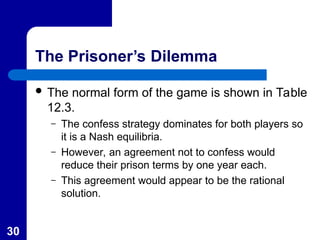
The Prisoner’s Dilemma
The normal form of the game is shown in Table
12.3.
– The confess strategy dominates for both players so
it is a Nash equilibria.
– However, an agreement not to confess would
reduce their prison terms by one year each.
– This agreement would appear to be the rational
solution.
31.
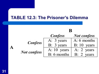
31
TABLE 12.3: ThePrisoner’s Dilemma
B
Confess Not confess
Confess
A: 3 years
B: 3 years
A: 6 months
B: 10 years
A
Not confess
A: 10 years
B: 6 months
A: 2 years
B: 2 years
32.
32
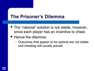
The Prisoner’s Dilemma
The “rational” solution is not stable, however,
since each player has an incentive to cheat.
Hence the dilemma:
– Outcomes that appear to be optimal are not stable
and cheating will usually prevail.
33.
33
Prisoner’s Dilemma Applications
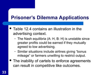
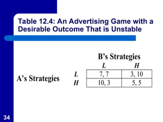
Table 12.4 contains an illustration in the
advertising context.
– The Nash equilibria (A: H, B: H) is unstable since
greater profits could be earned if they mutually
agreed to low advertising.
– Similar situations include airlines giving “bonus
mileage” or farmers unwilling to restrict output.
The inability of cartels to enforce agreements
can result in competitive like outcomes.
34.
34
Table 12.4: AnAdvertising Game with a
Desirable Outcome That is Unstable
B’s Strategies
L H
L 7, 7 3, 10
A’s Strategies H 10, 3 5, 5
35.
35
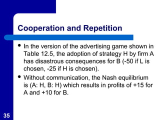
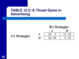
Cooperation and Repetition
In the version of the advertising game shown in
Table 12.5, the adoption of strategy H by firm A
has disastrous consequences for B (-50 if L is
chosen, -25 if H is chosen).
Without communication, the Nash equilibrium
is (A: H, B: H) which results in profits of +15 for
A and +10 for B.
36.
36
TABLE 12.5: AThreat Game in
Advertising
B’s Strategies
L H
L 20, 5 15, 10
A’s Strategies H 10, -50 5, -25
37.
37
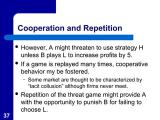
Cooperation and Repetition
However, A might threaten to use strategy H
unless B plays L to increase profits by 5.
If a game is replayed many times, cooperative
behavior my be fostered.
– Some market are thought to be characterized by
“tacit collusion” although firms never meet.
Repetition of the threat game might provide A
with the opportunity to punish B for failing to
choose L.
38.
38
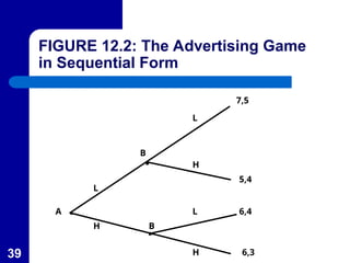
Many-Period Games
Figure12.2 repeats the advertising game
except that B knows which advertising
spending level A has chosen.
– The oral around B’s nodes has been eliminated.
B’s strategic choices now must be phrased in a
way that takes the added information into
account.
40
Many-Period Games
Thefour strategies for B are shown in Table
12.6.
– For example, the strategy (H, L) indicates that B
chooses L if A first chooses H.
The explicit considerations of contingent
strategy choices enables the exploration of
equilibrium notions in dynamic games.
41.
41
TABLE 12.6: ContingentStrategies in
the Advertising Game
B’s Strategies
L, L L, H H, L H, H
L 7, 5 7, 5 5, 4 5, 4
A’s Strategies H 6, 4 6, 3 6, 4 6, 3
42.
42
Credible Threat
Thethree Nash equilibria in the game shown in
Table 12.6 are:
– (1) A: L, B: (L, L);
– (2) A: L, B: (L, H); and
– (3) A: H, B: (H,L).
Pairs (2) and (3) are implausible, however,
because they incorporate a noncredible threat
that firm B would never carry out.
43.
43
Credible Threat
Consider,for example, A: L, B: (L, H) where B
promises to play H if A plays H.
– This threat is not credible (empty threats) since, if A
has chosen H, B would receive profits of 3 if it
chooses H but profits of 4 if it chooses L.
By eliminating strategies that involve
noncredible threats, A can conclude that, as
before, B would always play L.
44.
44
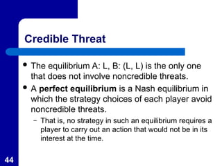
Credible Threat
Theequilibrium A: L, B: (L, L) is the only one
that does not involve noncredible threats.
A perfect equilibrium is a Nash equilibrium in
which the strategy choices of each player avoid
noncredible threats.
– That is, no strategy in such an equilibrium requires a
player to carry out an action that would not be in its
interest at the time.
45.
45
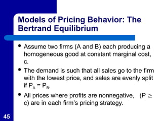
Models of PricingBehavior: The
Bertrand Equilibrium
Assume two firms (A and B) each producing a
homogeneous good at constant marginal cost,
c.
The demand is such that all sales go to the firm
with the lowest price, and sales are evenly split
if PA = PB.
All prices where profits are nonnegative, (P
c) are in each firm’s pricing strategy.
46.
46
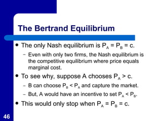
The Bertrand Equilibrium
The only Nash equilibrium is PA = PB = c.
– Even with only two firms, the Nash equilibrium is
the competitive equilibrium where price equals
marginal cost.
To see why, suppose A chooses PA > c.
– B can choose PB < PA and capture the market.
– But, A would have an incentive to set PA < PB.
This would only stop when PA = PB = c.
47.
47
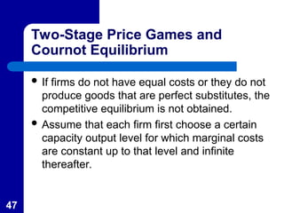
Two-Stage Price Gamesand
Cournot Equilibrium
If firms do not have equal costs or they do not
produce goods that are perfect substitutes, the
competitive equilibrium is not obtained.
Assume that each firm first choose a certain
capacity output level for which marginal costs
are constant up to that level and infinite
thereafter.
48.
48
Two-Stage Price Gamesand
Cournot Equilibrium
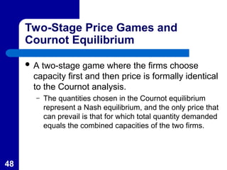
A two-stage game where the firms choose
capacity first and then price is formally identical
to the Cournot analysis.
– The quantities chosen in the Cournot equilibrium
represent a Nash equilibrium, and the only price that
can prevail is that for which total quantity demanded
equals the combined capacities of the two firms.
49.
49
Two-Stage Price Gamesand
Cournot Equilibrium
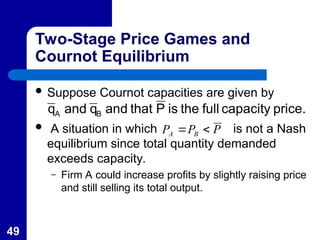
Suppose Cournot capacities are given by
A situation in which is not a Nash
equilibrium since total quantity demanded
exceeds capacity.
– Firm A could increase profits by slightly raising price
and still selling its total output.
price.
capacity
full
the
is
P
that
and
q
and
q B
A
P
P
P B
A
50.
50
Two-Stage Price Gamesand
Cournot Equilibrium
P
P
P B
A
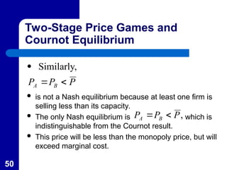
Similarly,
is not a Nash equilibrium because at least one firm is
selling less than its capacity.
The only Nash equilibrium is which is
indistinguishable from the Cournot result.
This price will be less than the monopoly price, but will
exceed marginal cost.
,
P
P
P B
A
51.
51
Comparing the Bertrandand
Cournot Results
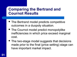
The Bertrand model predicts competitive
outcomes in a duopoly situation.
The Cournot model predict monopolylike
inefficiencies in which price exceed marginal
cost.
The two-stage model suggests that decisions
made prior to the final (price setting) stage can
have important market impact.
52.
52
APPLICATION 12.2: Howis the Price
Game Played?
Many factors influence how the pricing “game”
is played in imperfectly competitive industries.
Two such factors that have been examined
are
– Product Availability
– Information Sharing
53.
53
APPLICATION 12.2: Howis the Price
Game Played?
Product availability is an important component of
competition in many retail industries.
The impact of movie availability in the video-rental
industry was examined in 2001 by James Dana.
His data showed that Blockbuster’s prices were 40%
higher than at other stores.
He argued that Blockbuster’s higher price in part stems
from its reputation for having movies available and that
those prices act as a signal.
54.
54
APPLICATION 12.2: Howis the Price
Game Played?
Firms in the same industry often share information with
each other at many levels.
A 2000 study of cross-shareholding in the Dutch
financial sector showed clear evidence that competition
was reduced when firms had financial interests in each
other’s profits.
A famous 1914 antitrust case found that a price list
published by lumber retailers facilitated higher prices
by discouraging wholesalers from selling at retail.
55.
55
Tacit Collusion: FiniteTime Horizon
Would the single-period Nash equilibrium in the
Bertrand model, PA = PB = c, change if the
game were repeated during many periods?
– With a finite period, any strategy in which firm A,
say, chooses, PA > c in the last period offers B the
possibility of earning profits by setting PA > PB > c.
56.
56
Tacit Collusion: FiniteTime Horizon
– The threat of charging PA > c in the last period is not
credible.
– A similar argument is applicable for any period
before the last period.
The only perfect equilibrium requires firms
charge the competitive price in all periods.
Tacit collusion is impossible over a finite
period.
57.
57
Tacit Collusion: InfiniteTime
Horizon
Without a “final” period, there may exist
collusive strategies.
– One possibility is a “trigger” strategy where each
firm sets its price at the monopoly price so long as
the other firm adopts a similar price.
If one firm sets a lower price in any period, the other firm
sets its price equal to marginal cost in the subsequent
period.
58.
58
Tacit Collusion: InfiniteTime
Horizon
Suppose the firms collude for a time and firm A
considers cheating in this period.
– Firm B will set PB = PM (the cartel price)
– A can set its price slightly lower and capture the
entire market.
– Firm A will earn (almost) the entire monopoly profit
(M) in this period.
59.
59
Tacit Collusion: InfiniteTime
Horizon
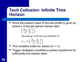
Since the present value of the lost profits is given by
(where r is the per period interest rate)
This condition holds for values of r < ½.
Trigger strategies constitute a perfect equilibrium for
sufficiently low interest rates.
.
1
2
if
profitable
be
will
cheating
,
1
2
r
r
M
M
M
60.
60
Generalizations and Limitations
Assumptions of the tacit collusion model:
– Firm B can easily detect whether firm A has cheated
– Firm B responds to cheating by adopting a harsh
response that punishes firm A, and condemns itself
to zero profit forever.
More general models relax one or both of
these assumptions with varying results.
61.
61
APPLICATION 12.3: TheGreat
Electrical Equipment Conspiracy
Manufacturing of electric turbine generators
and high voltage switching units provided a
very lucrative business to such major
producers and General Electric, Westinghouse,
and Federal Pacific Corporations after World
War II.
However, the prospect of possible monopoly
profits proved enticing.
62.
62
APPLICATION 12.3: TheGreat
Electrical Equipment Conspiracy
To collude they had to create a method to
coordinate their sealed bids.
– This was accomplished through dividing the country
into bidding regions and using the lunar calendar to
decide who would “win” a bid.
The conspiracy became more difficult as its
leaders had to give greater shares to other
firms toward the end of the 1950s.
63.
63
APPLICATION 12.3: TheGreat
Electrical Equipment Conspiracy
The conspiracy was exposed when a
newspaper reporter discovered that some of
the bids on Tennessee Valley Authority
projects were similar.
Federal indictments of 52 executives lead to
jail time for some and resulted in a chilling
effect on the future establishment of other
cartels of this type.
64.
64
Entry, Exit, andStrategy
Sunk Costs
– Expenditures that once made cannot be recovered
include expenditures on unique types of equipment
or job-specific training.
– These costs are incurred only once as part of the
entry process.
– Such entry investments mean the firm has a
commitment to the market.
65.
65
First-Mover Advantages
Thecommitment of the first firm into a market
may limit the kinds of actions rivals find
profitable.
Using the Cournot model of water springs,
suppose firm A can move first.
– It will take into consideration what firm B will do to
maximize profits given what firm A has already
done.
66.
66
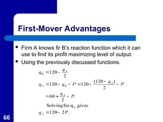
First-Mover Advantages
FirmA knows fir B’s reaction function which it can
use to find its profit maximizing level of output.
Using the previously discussed functions.
.
2
120
gives
q
for
Solving
.
2
60
2
)
120
(
120
120
2
120
A
P
q
P
q
P
q
P
q
q
q
q
A
A
A
B
A
A
B
67.
67
First-Mover Advantages
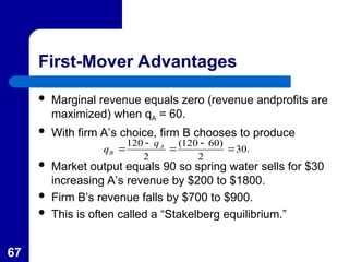
Marginalrevenue equals zero (revenue andprofits are
maximized) when qA = 60.
With firm A’s choice, firm B chooses to produce
Market output equals 90 so spring water sells for $30
increasing A’s revenue by $200 to $1800.
Firm B’s revenue falls by $700 to $900.
This is often called a “Stakelberg equilibrium.”
.
30
2
)
60
120
(
2
120
A
B
q
q
68.
68
Entry Deterrence
Inthe previous model, firm A could only deter
firm B from entering the market if it produces
the full market output of 120 units yielding zero
revenue (since P = $0).
With economies of scale, however, it may be
possible for a first-mover to limit the scale of
operation of a potential entrant and deter all
entry into the market.
69.
69
A Numerical Example
One simple way to incorporate economies of
scale is to have fixed costs.
Using the previous model, assume each firm
has to pay fixed cost of $784.
– If firm A produced 60, firm B would earn profits of
$116 (= $900 - $784) per period.
– If firm A produced 64, firm B would choose to
produce 28 [ = (120-64) 2].
70.
70
A Numerical Example
–Total output would equal 92 with P = $28.
– Firm B’s profits equal zero [profits = TR - TC =
($28·28) - $784 = 0] so it would not enter.
– Firm A would choose a price of $56 (= 120 - 64)
and earn profits of $2,800 [= ($56·64) - $784].
Economies of scale along with the chance to
be the first mover yield a profitable entry
deterrence.
71.
71
APPLICATION 12.4: First-MoverAdvantages for
Alcoa, DuPont, Procter and Gamble, and Wal-Mart
Consider two types of first-mover advantages
– Advantages that stem from economies of scale in
production.
– Advantages that arise in connection with the
introduction of pioneering brands.
72.
72
APPLICATION 12.4: First-MoverAdvantages for
Alcoa, DuPont, Procter and Gamble, and Wal-Mart
Economies of Scale for Alcoa and DuPont.
– The first firm in the market may “overbuild” its initial
plant to realize economies of scale when the
demand for the product expands.
– Antitrust action against the Aluminum Company of
America (Alcoa) claimed that it built larger plants
than justified by current demand.
73.
73
APPLICATION 12.4: First-MoverAdvantages for
Alcoa, DuPont, Procter and Gamble, and Wal-Mart
– In the 1970s, DuPont expanded its capacity to
produce titanium dioxide which is a primary coloring
agent in white paint.
– Studies suggest that this strategy was successful in
forestalling new investment by others into the
titanium dioxide market.
74.
74
APPLICATION 12.4: First-MoverAdvantages for
Alcoa, DuPont, Procter and Gamble, and Wal-Mart
Pioneering Brands for Proctor and Gamble
– Introducing the first brand of a new product
appears to provide considerable advantage over
later-arriving rivals.
– Proctor and Gamble was successful in this with
Tide laundry detergent in the 1940s and Crest
toothpaste in the 1950s.
– New products are a risk for consumers, and if the
first one works, consumers may stick with it.
75.
75
APPLICATION 12.4: First-MoverAdvantages for
Alcoa, DuPont, Procter and Gamble, and Wal-Mart
The Wal-Mart Advantage
– Its success stems from its first mover advantage in
economies of scale and its initial “small town”
strategy.
– Started in the 1960s, it started serving smaller,
mostly Southern markets.
– This profitable near monopoly situation allowed it to
grow and gain economies of scale in distribution
and in buying power.
76.
76
Limit Pricing
Alimit price is a situation where a
monopoly might purposely choose a low
(“limit”) price policy with a goal of deterring
entry into its market.
– If an incumbent monopoly chooses a price
PL < PM (the profit-maximizing price) it is
hurting its current profits.
– PL will deter entry only if it falls short of the
average cost of a potential entrant.
77.
77
Limit Pricing
– Ifthe monopoly and potential entrant have the
same costs (and there are no capacity
constraints), the only limit price is PL = AC, which
results in zero economic profits.
Hence, the basic monopoly model does not
provide a mechanism for limit pricing to work.
Thus, a limit price model must depart from
traditional assumptions.
78.
78
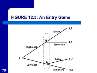
Incomplete Information
Ifan incumbent monopoly knows more about
the market than a potential entrant, it may be
able to use this knowledge to deter entry.
Consider Figure 12.3.
– Firm A, the incumbent monopolist, may have “high”
or “low” production costs based on past decisions
which are unknown to firm B.
80
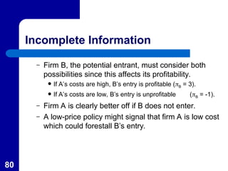
Incomplete Information
– FirmB, the potential entrant, must consider both
possibilities since this affects its profitability.
If A’s costs are high, B’s entry is profitable (B = 3).
If A’s costs are low, B’s entry is unprofitable (B = -1).
– Firm A is clearly better off if B does not enter.
– A low-price policy might signal that firm A is low cost
which could forestall B’s entry.
81.
81
Predatory Pricing
Thestructure of many predatory pricing
models also stress asymmetric information.
An incumbent firm wishes its rival would exit
the market so it takes actions to affect the
rival’s view of future profitability.
As with limit pricing, the success depends on
the ability of the monopoly to take advantage
of its better information.
82.
82
Predatory Pricing
Possiblestrategies include:
– Signal low costs with a low-price policy.
– Adopt extensive production differentiation to indicate
the existence of economies of scale.
Once a rival is convinced the incumbent firm
possess an advantage, it may exit the market,
and the incumbent gains monopoly profits.
83.
83
APPLICATION 12.4: TheStandard Oil
Legend
The Standard Oil case of 1911 was one of the
landmarks of U.S. antitrust law.
In that case, Standard Oil Company was found to have
“attempted to monopolize” the production, refining, and
distribution of petroleum in the U.S., violating the
Sherman Act.
The government claimed that the company would cut
prices dramatically to drive rivals out of a particular
market and then raise prices back to monopoly levels.
84.
84
APPLICATION 12.4: TheStandard Oil
Legend
Unfortunately, the notion that Standard Oil practiced
predatory pricing policies in order to discourage entry
and encourage exit by its rivals makes little sense in
terms of economic theory.
Actually, the predator would have to operate with
relatively large losses for some time in the hope that
the smaller losses this may cause rivals will eventually
prompt them to give it up.
This strategy is clearly inferior to the strategy of simply
buying smaller rivals in the marketplace.
85.
85
APPLICATION 12.4: TheStandard Oil
Legend
In a famous 1958 article, J.S. McGee concluded that
Standard Oil neither trieds to use predatory policies nor
did its actual price policies have the effect of driving
rivals from the oil business.
McGee examined over 100 refineries bought by
Standard Oil and found no evidence that predatory
behavior by Standard Oil caused these firms to sell out.
Indeed, in many cases Standard Oil paid quite good
prices for these refineries.
86.
86
N-Player Game Theory
The most important additional element added
when the game goes beyond two players is the
possibility for the formation of subsets of
players.
Coalitions are combinations of two or more
players in a game who adopt coordinated
strategies.
– A two-person game example is a cartel.
87.
87
N-Player Game Theory
The formation of successful coalitions in n-
player games if influenced by organizational
costs.
– Information costs associated with determining
coalition strategies.
– Enforcement costs associated with ensuring that a
coalition’s chosen strategy is actually followed by its
members.


![69
A Numerical Example
One simple way to incorporate economies of
scale is to have fixed costs.
Using the previous model, assume each firm
has to pay fixed cost of $784.
– If firm A produced 60, firm B would earn profits of
$116 (= $900 - $784) per period.
– If firm A produced 64, firm B would choose to
produce 28 [ = (120-64) 2].](https://image.slidesharecdn.com/kloppstrategyandgametheory-250811055058-49d11d54/85/KLOPP-Strategy-and-Game-Theory-ppt-explained-69-320.jpg)
![70
A Numerical Example
– Total output would equal 92 with P = $28.
– Firm B’s profits equal zero [profits = TR - TC =
($28·28) - $784 = 0] so it would not enter.
– Firm A would choose a price of $56 (= 120 - 64)
and earn profits of $2,800 [= ($56·64) - $784].
Economies of scale along with the chance to
be the first mover yield a profitable entry
deterrence.](https://image.slidesharecdn.com/kloppstrategyandgametheory-250811055058-49d11d54/85/KLOPP-Strategy-and-Game-Theory-ppt-explained-70-320.jpg)