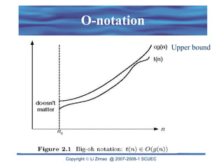
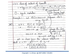
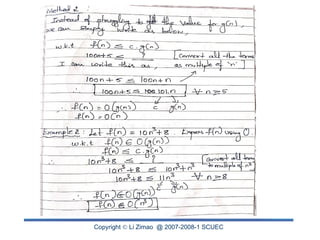
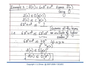
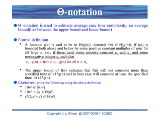
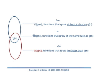
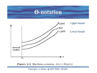
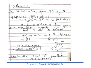
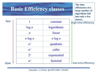
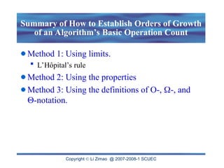
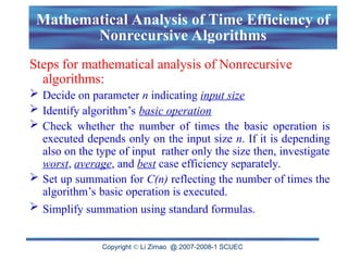
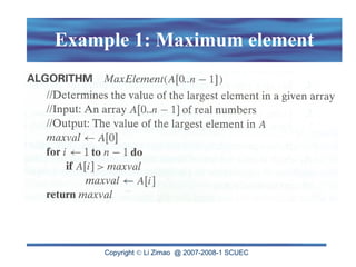
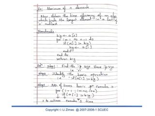
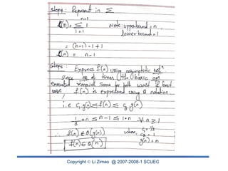
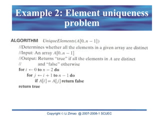
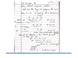
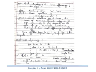
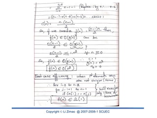
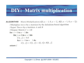
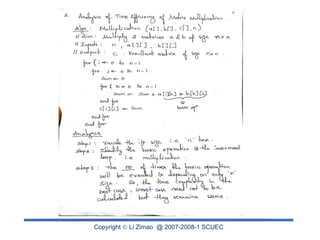
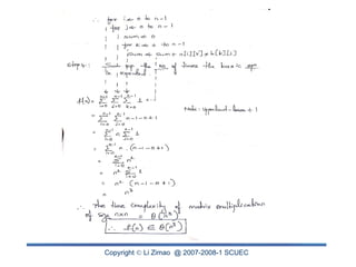
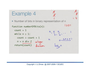
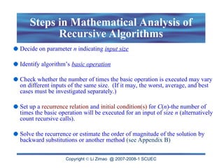
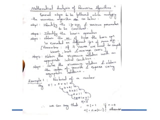
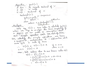
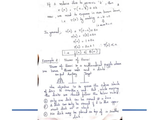
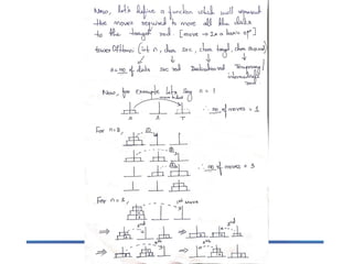
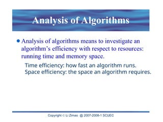
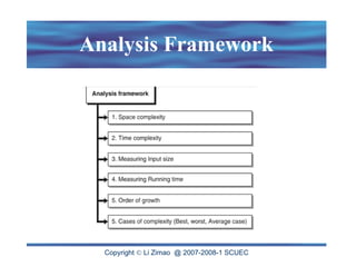
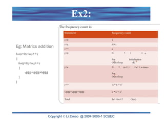
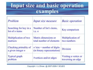
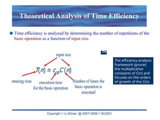
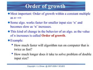
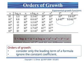
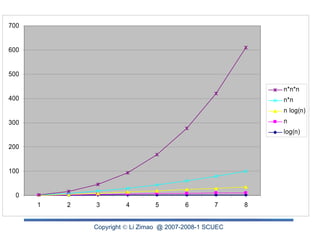
The document discusses the analysis of algorithm efficiency focusing on time and space complexities, and how these are affected by input size and algorithm choice. It details methods for measuring running time, including the basic operation of algorithms and different cases of efficiency (worst, best, and average). Furthermore, it introduces asymptotic notations (O, Ω, Θ) to classify and compare the growth rates of algorithms and their order of complexity.

![Copyright Li Zimao @ 2007-2008-1 SCUEC
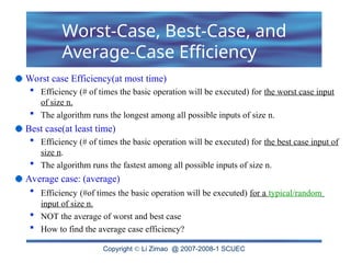
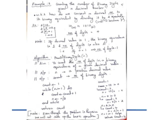
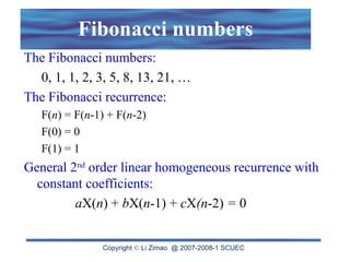
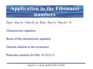
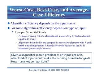
Sequential Search Algorithm
ALGORITHM SequentialSearch(A[0..n-1], K)
//Searches for a given value in a given array by sequential search
//Input: An array A[0..n-1] and a search key K
//Output: Returns the index of the first element of A that matches K or –1 if there
are no matching elements
i 0
while i < n and A[i] ‡ K do
i i + 1
if i < n //A[I] = K
return i
else
return -1](https://image.slidesharecdn.com/3-240918163411-c42ba3cf/85/3-analysis-of-algorithms-efficiency-ppt-15-320.jpg)