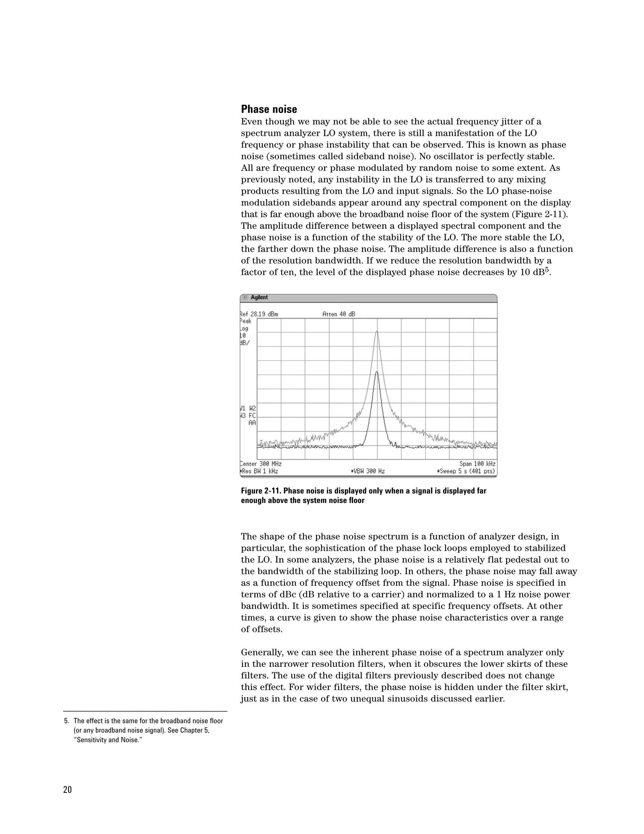
Downloaded 91 times
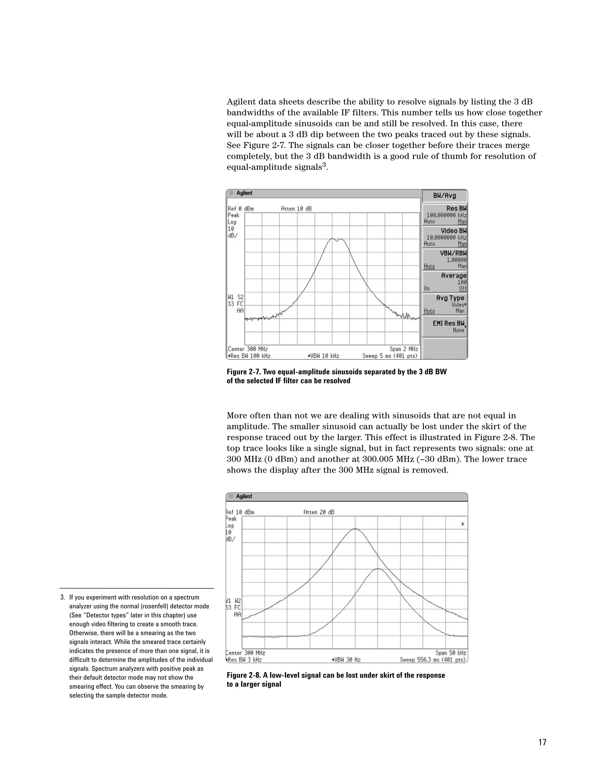
![Another specification is listed for the resolution filters: bandwidth selectivity
(or selectivity or shape factor). Bandwidth selectivity helps determine the
resolving power for unequal sinusoids. For Agilent analyzers, bandwidth
selectivity is generally specified as the ratio of the 60 dB bandwidth to the
3 dB bandwidth, as shown in Figure 2-9. The analog filters in Agilent analyzers
are a four-pole, synchronously-tuned design, with a nearly Gaussian shape4.
This type of filter exhibits a bandwidth selectivity of about 12.7:1.
3 dB
60 dB
Figure 2-9. Bandwidth selectivity, ratio of 60 dB to 3 dB bandwidths
For example, what resolution bandwidth must we choose to resolve signals
that differ by 4 kHz and 30 dB, assuming 12.7:1 bandwidth selectivity? Since
we are concerned with rejection of the larger signal when the analyzer is
tuned to the smaller signal, we need to consider not the full bandwidth, but
the frequency difference from the filter center frequency to the skirt. To
determine how far down the filter skirt is at a given offset, we use the
following equation:
H(∆f) = –10(N) log10 [(∆f/f0)2 + 1]
Where H(∆f) is the filter skirt rejection in dB
N is the number of filter poles
∆f is the frequency offset from the center in Hz, and
RBW
f0 is given by
2 √ 21/N –1
For our example, N=4 and ∆f = 4000. Let’s begin by trying the 3 kHz RBW
filter. First, we compute f0:
3000
f0 = = 3448.44
2 √ 21/4 –1
Now we can determine the filter rejection at a 4 kHz offset:
4. Some older spectrum analyzer models used five-pole H(4000) = –10(4) log10 [(4000/3448.44)2 + 1]
filters for the narrowest resolution bandwidths to = –14.8 dB
provide improved selectivity of about 10:1. Modern
designs achieve even better bandwidth selectivity This is not enough to allow us to see the smaller signal. Let’s determine H(∆f)
using digital IF filters.
again using a 1 kHz filter:
1000
f0 = = 1149.48
2 √ 21/4 –1
18](https://image.slidesharecdn.com/2259filespectrumanalysisbasicsapplicationnote150aligent2005-120408110648-phpapp02/75/2259-file-spectrum_analysis_basics_application_note_150_aligent_2005-18-2048.jpg)
![This allows us to calculate the filter rejection:
H(4000) = –10(4) log10[(4000/1149.48)2 + 1]
= –44.7 dB
Thus, the 1 kHz resolution bandwidth filter does resolve the smaller signal.
This is illustrated in Figure 2-10.
Figure 2-10. The 3 kHz filter (top trace) does not resolve smaller signal;
reducing the resolution bandwidth to 1 kHz (bottom trace) does
Digital filters
Some spectrum analyzers use digital techniques to realize their resolution
bandwidth filters. Digital filters can provide important benefits, such
as dramatically improved bandwidth selectivity. The Agilent PSA Series
spectrum analyzers implement all resolution bandwidths digitally. Other
analyzers, such as the Agilent ESA-E Series, take a hybrid approach, using
analog filters for the wider bandwidths and digital filters for bandwidths of
300 Hz and below. Refer to Chapter 3 for more information on digital filters.
Residual FM
Filter bandwidth is not the only factor that affects the resolution of a
spectrum analyzer. The stability of the LOs in the analyzer, particularly the
first LO, also affects resolution. The first LO is typically a YIG-tuned oscillator
(tuning somewhere in the 3 to 7 GHz range). In early spectrum analyzer
designs, these oscillators had residual FM of 1 kHz or more. This instability
was transferred to any mixing products resulting from the LO and incoming
signals, and it was not possible to determine whether the input signal or the
LO was the source of this instability.
The minimum resolution bandwidth is determined, at least in part, by the
stability of the first LO. Analyzers where no steps are taken to improve upon
the inherent residual FM of the YIG oscillators typically have a minimum
bandwidth of 1 kHz. However, modern analyzers have dramatically improved
residual FM. For example, Agilent PSA Series analyzers have residual FM of
1 to 4 Hz and ESA Series analyzers have 2 to 8 Hz residual FM. This allows
bandwidths as low as 1 Hz. So any instability we see on a spectrum analyzer
today is due to the incoming signal.
19](https://image.slidesharecdn.com/2259filespectrumanalysisbasicsapplicationnote150aligent2005-120408110648-phpapp02/75/2259-file-spectrum_analysis_basics_application_note_150_aligent_2005-19-2048.jpg)
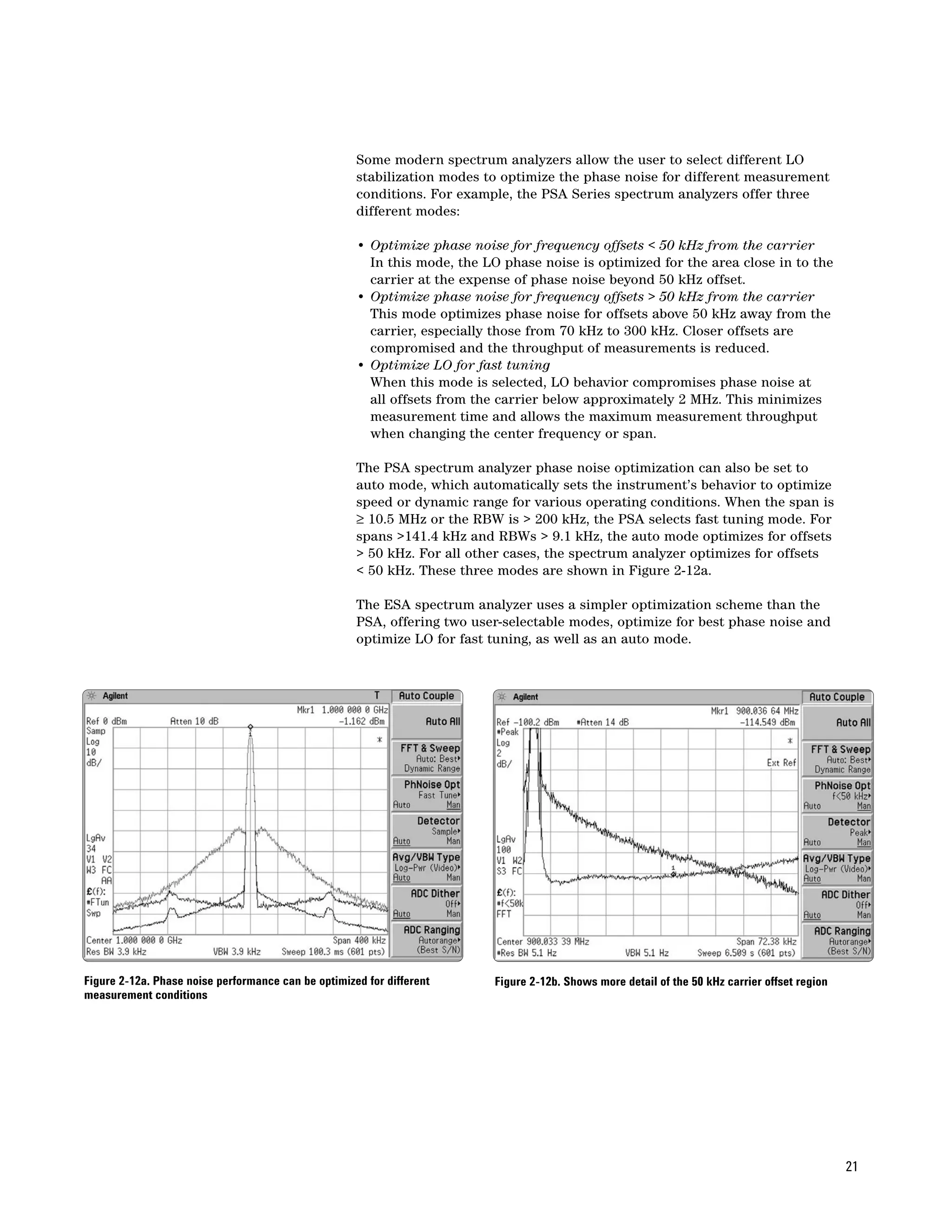
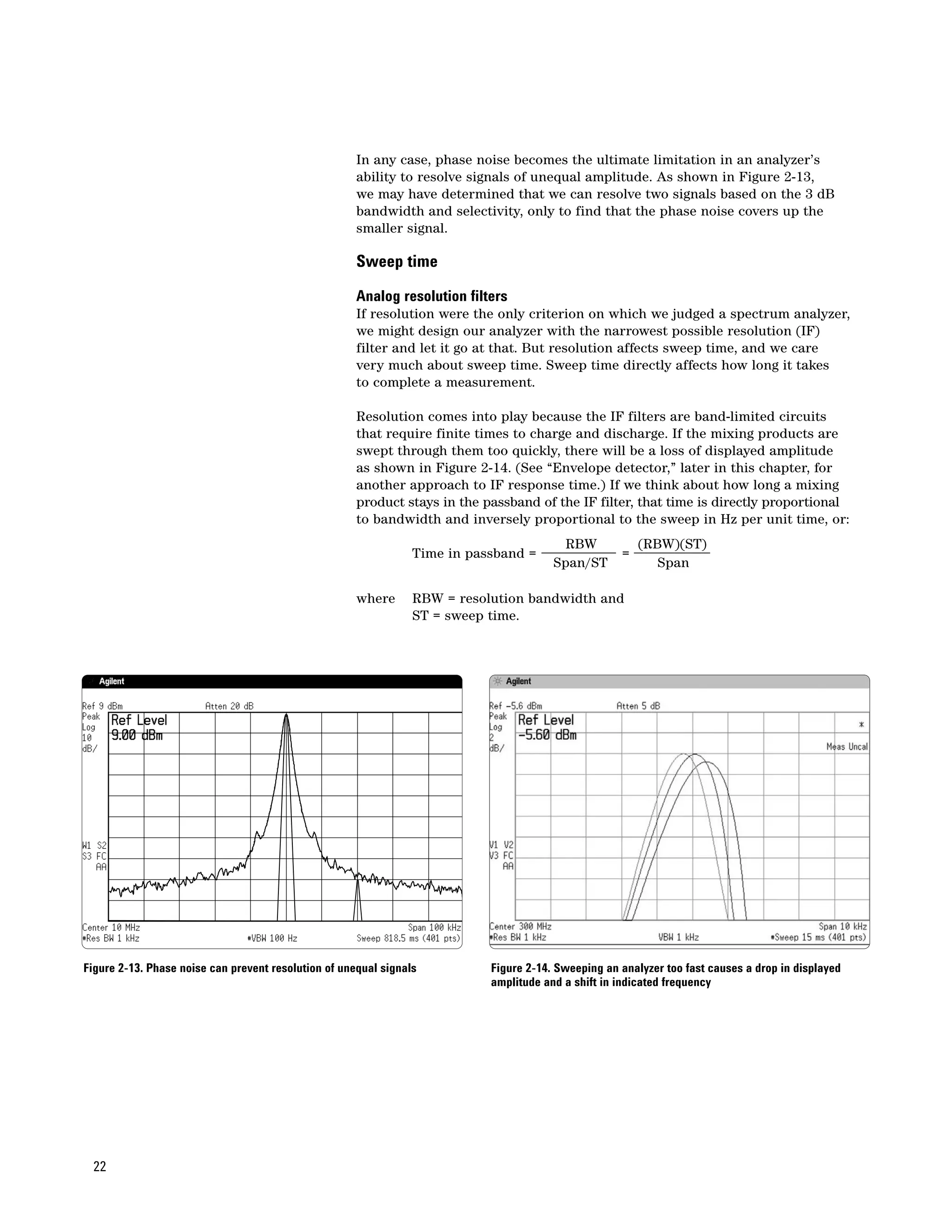
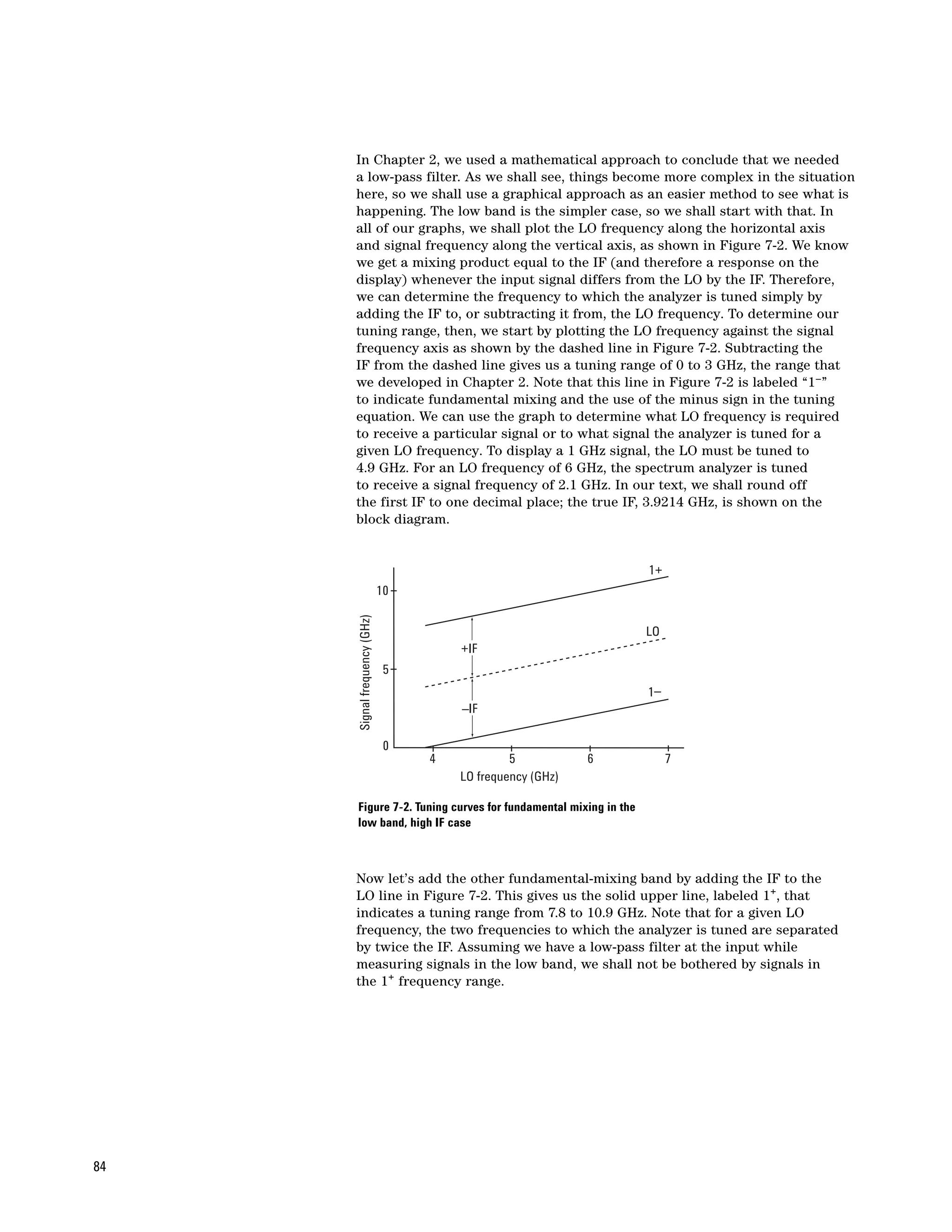
![In Chapter 2, we did a filter skirt selectivity calculation for two signals
spaced 4 kHz apart, using a 3 kHz analog filter. Let’s repeat that calculation
using digital filters. A good model of the selectivity of digital filters is a
near-Gaussian model:
∆f α
H(∆f) = –3.01 dB x
RBW/2 [ ]
where H(∆f) is the filter skirt rejection in dB
∆f is the frequency offset from the center in Hz, and
α is a parameter that controls selectivity. α = 2 for an ideal
Gaussian filter. The swept RBW filters used in Agilent
spectrum analyzers are based on a near-Gaussian model with an α
value equal to 2.12, resulting in a selectivity ratio of 4.1:1.
Entering the values from our example into the equation, we get:
4000 2.12
H(4 kHz) = –3.01 dB x [ 3000/2 ]
= –24.1 dB
At an offset of 4 kHz, the 3 kHz digital filter is down –24.1 dB compared
to the analog filter which was only down –14.8 dB. Because of its superior
selectivity, the digital filter can resolve more closely spaced signals.
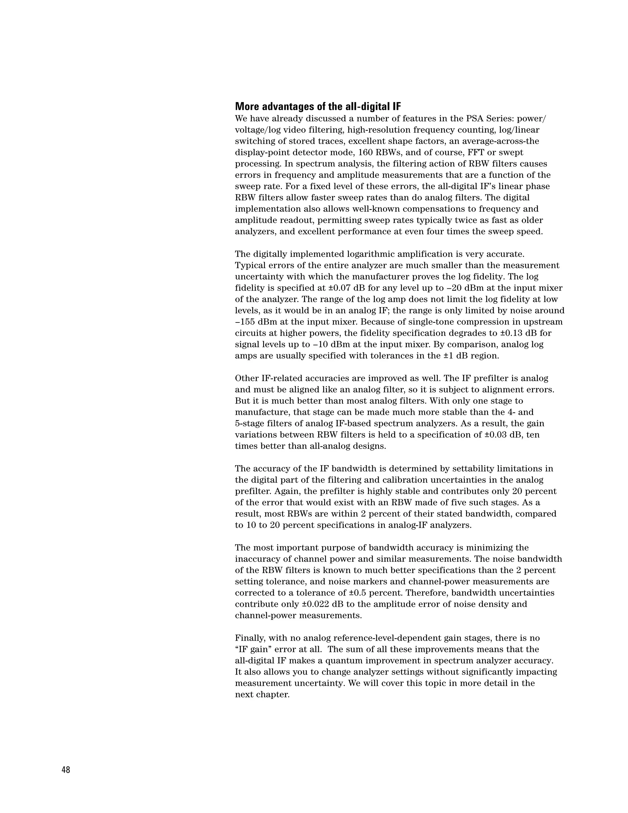
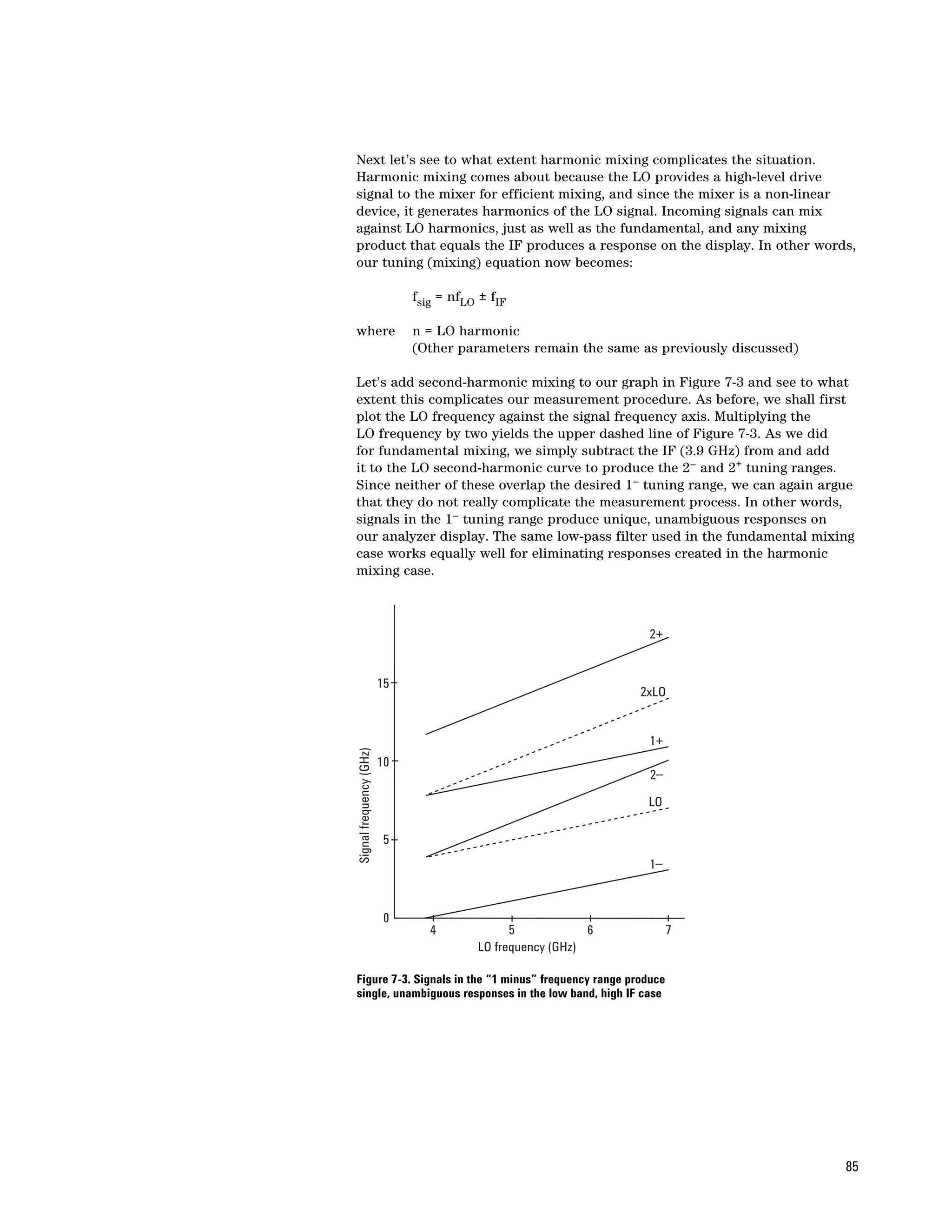
The all-digital IF
The Agilent PSA Series spectrum analyzers have, for the first time, combined
several digital techniques to achieve the all-digital IF. The all-digital IF brings
a wealth of advantages to the user. The combination of FFT analysis for
narrow spans and swept analysis for wider spans optimizes sweeps for the
fastest possible measurements. Architecturally, the ADC is moved closer
to the input port, a move made possible by improvements to the A-to-D
converters and other digital hardware. Let’s begin by taking a look at the
block diagram of the all-digital IF in the PSA spectrum analyzer, as shown
in Figure 3-2.
Custom IC
Anti-alias Counter
I
filter
I, Q Display
ADC VBW det
Q log (r)
r,
log pwr pwr log
Hilbert log v v log
Ranging -1 transform
Prefilter rules log log log log
Autoranging ADC system
RISC processor
Display
FFT Processing
log/lin dB/div Display
Figure 3-2. Block diagram of the all-digital IF in the Agilent PSA Series
45](https://image.slidesharecdn.com/2259filespectrumanalysisbasicsapplicationnote150aligent2005-120408110648-phpapp02/75/2259-file-spectrum_analysis_basics_application_note_150_aligent_2005-45-2048.jpg)
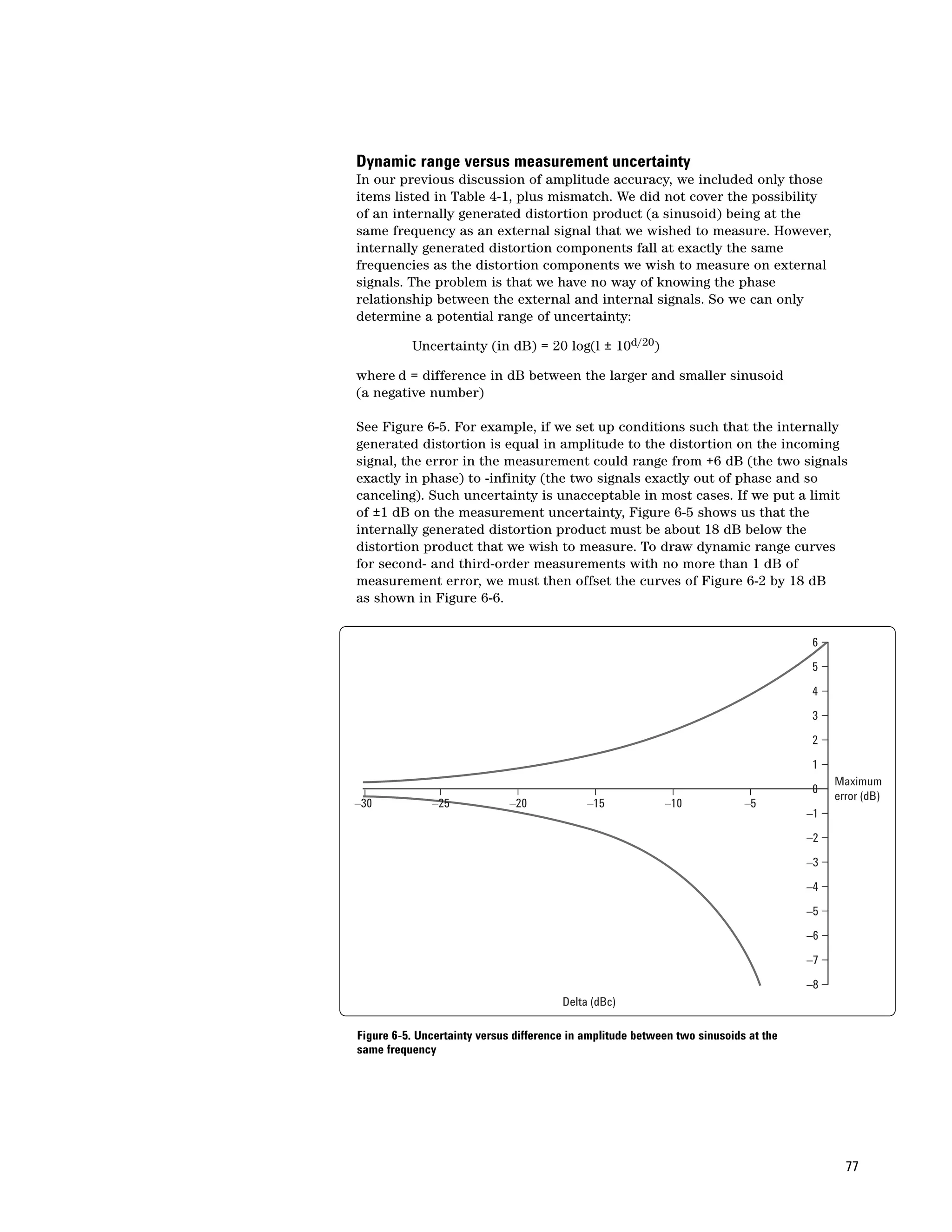
![The general expression used to calculate the maximum mismatch error
in dB is:
Error (dB) = –20 log[1 ± |(ρanalyzer)(ρsource)|]
where ρ is the reflection coefficient
Spectrum analyzer data sheets typically specify the input voltage standing
wave ratio (VSWR). Knowing the VSWR, we can calculate ρ with the following
equation:
(VSWR–1)
ρ=
(VSWR+1)
As an example, consider a spectrum analyzer with an input VSWR of 1.2 and
a device under test (DUT) with a VSWR of 1.4 at its output port. The resulting
mismatch error would be ±0.13 dB.
Since the analyzer’s worst-case match occurs when its input attenuator is
set to 0 dB, we should avoid the 0 dB setting if we can. Alternatively, we can
attach a well-matched pad (attenuator) to the analyzer input and greatly
reduce mismatch as a factor. Adding attenuation is a technique that works
well to reduce measurement uncertainty when the signal we wish to measure
is well above the noise. However, in cases where the signal-to-noise ratio is
small (typically ≤7 dB), adding attenuation will increase measurement error
because the noise power adds to the signal power, resulting in an erroneously
high reading.
Let’s turn our attention to the input attenuator. Some relative measurements
are made with different attenuator settings. In these cases, we must consider
the input attenuation switching uncertainty. Because an RF input
attenuator must operate over the entire frequency range of the analyzer,
its step accuracy varies with frequency. The attenuator also contributes
to the overall frequency response. At 1 GHz, we expect the attenuator
performance to be quite good; at 26 GHz, not as good.
The next component in the signal path is the input filter. Spectrum analyzers
use a fixed low-pass filter in the low band and a tunable band pass filter
called a preselector (we will discuss the preselector in more detail in
Chapter 7) in the higher frequency bands. The low-pass filter has a better
frequency response than the preselector and adds a small amount of
uncertainty to the frequency response error. A preselector, usually a
YIG-tuned filter, has a larger frequency response variation, ranging from
1.5 dB to 3 dB at millimeter-wave frequencies.
50](https://image.slidesharecdn.com/2259filespectrumanalysisbasicsapplicationnote150aligent2005-120408110648-phpapp02/75/2259-file-spectrum_analysis_basics_application_note_150_aligent_2005-50-2048.jpg)

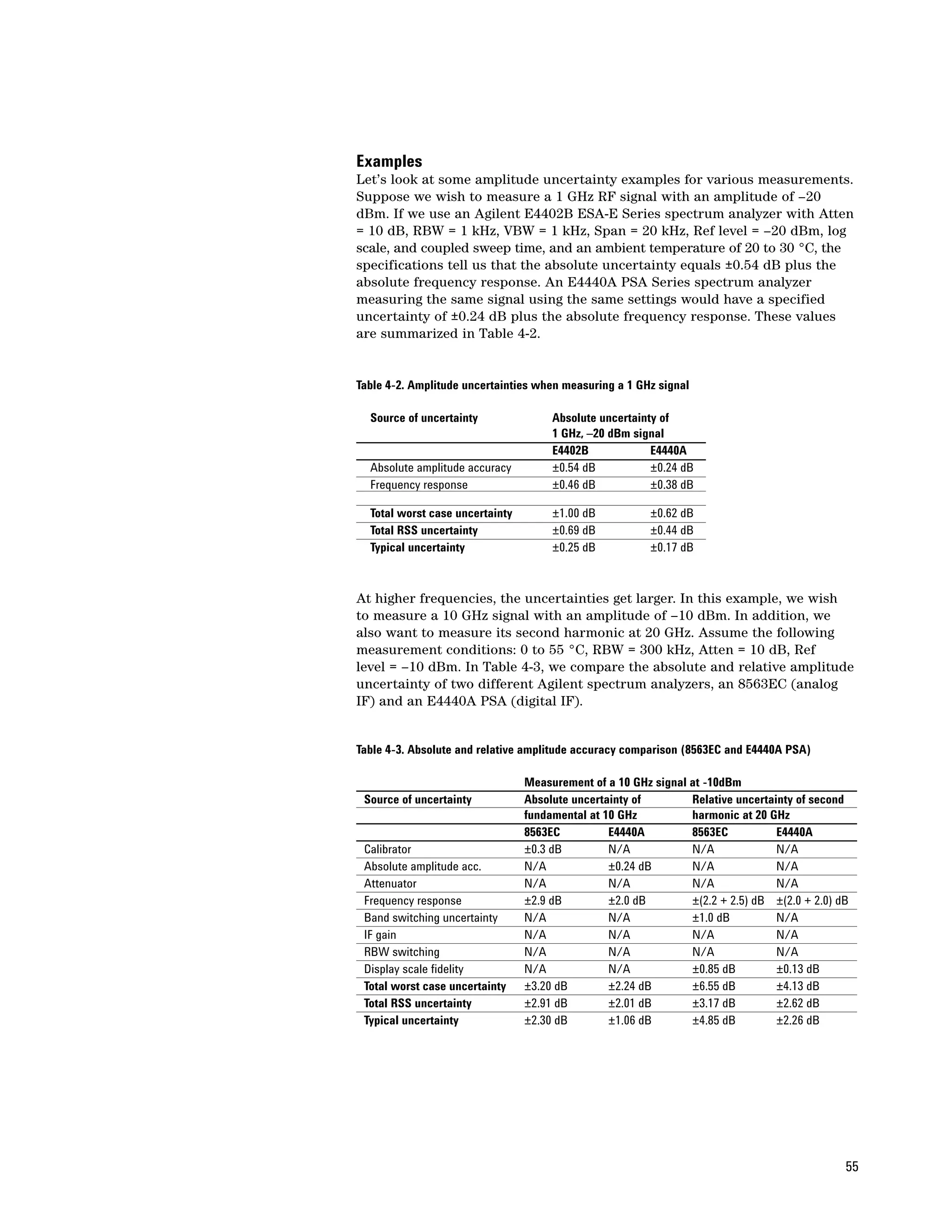
![Frequency accuracy
So far, we have focused almost exclusively on amplitude measurements.
What about frequency measurements? Again, we can classify two broad
categories, absolute and relative frequency measurements. Absolute
measurements are used to measure the frequencies of specific signals.
For example, we might want to measure a radio broadcast signal to verify
that it is operating at its assigned frequency. Absolute measurements are also
used to analyze undesired signals, such as when doing a spur search. Relative
measurements, on the other hand, are useful to know how far apart spectral
components are, or what the modulation frequency is.
Up until the late 1970s, absolute frequency uncertainty was measured in
megahertz because the first LO was a high-frequency oscillator operating
above the RF range of the analyzer, and there was no attempt to tie the LO to
a more accurate reference oscillator. Today’s LOs are synthesized to provide
better accuracy. Absolute frequency uncertainty is often described under
the frequency readout accuracy specification and refers to center frequency,
start, stop, and marker frequencies.
With the introduction of the Agilent 8568A in 1977, counter-like frequency
accuracy became available in a general-purpose spectrum analyzer and
ovenized oscillators were used to reduce drift. Over the years, crystal
reference oscillators with various forms of indirect synthesis have been
added to analyzers in all cost ranges. The broadest definition of indirect
synthesis is that the frequency of the oscillator in question is in some way
determined by a reference oscillator. This includes techniques such as phase
lock, frequency discrimination, and counter lock.
What we really care about is the effect these changes have had on frequency
accuracy (and drift). A typical readout accuracy might be stated as follows:
±[(freq readout x freq ref error) + A% of span + B% of RBW + C Hz]
Note that we cannot determine an exact frequency error unless we know
something about the frequency reference. In most cases we are given an
annual aging rate, such as ±1 x 10⁻⁷ per year, though sometimes aging is
given over a shorter period (for example, ±5 x 10⁻¹⁰ per day). In addition,
we need to know when the oscillator was last adjusted and how close it was
set to its nominal frequency (usually 10 MHz). Other factors that we often
overlook when we think about frequency accuracy include how long the
reference oscillator has been operating. Many oscillators take 24 to 72 hours
to reach their specified drift rate. To minimize this effect, some spectrum
analyzers continue to provide power to the reference oscillator as long as the
instrument is plugged into the AC power line. In this case, the instrument is
not really turned “off,” but more properly is on “standby.” We also need to
consider the temperature stability, as it can be worse than the drift rate.
In short, there are a number of factors to consider before we can determine
frequency uncertainty.
56](https://image.slidesharecdn.com/2259filespectrumanalysisbasicsapplicationnote150aligent2005-120408110648-phpapp02/75/2259-file-spectrum_analysis_basics_application_note_150_aligent_2005-56-2048.jpg)
![In a factory setting, there is often an in-house frequency standard available
that is traceable to a national standard. Most analyzers with internal
reference oscillators allow you to use an external reference. The frequency
reference error in the foregoing expression then becomes the error of the
in-house standard.
When making relative measurements, span accuracy comes into play.
For Agilent analyzers, span accuracy generally means the uncertainty in
the indicated separation of any two spectral components on the display.
For example, suppose span accuracy is 0.5% of span and we have two signals
separated by two divisions in a 1 MHz span (100 kHz per division). The
uncertainty of the signal separation would be 5 kHz. The uncertainty would
be the same if we used delta markers and the delta reading would be 200 kHz.
So we would measure 200 kHz ±5 kHz.
When making measurements in the field, we typically want to turn our
analyzer on, complete our task, and move on as quickly as possible. It is
helpful to know how the reference in our analyzer behaves under short warm
up conditions. For example, the Agilent ESA-E Series of portable spectrum
analyzers will meet published specifications after a five-minute warm up time.
Most analyzers include markers that can be put on a signal to give us
absolute frequency, as well as amplitude. However, the indicated frequency
of the marker is a function of the frequency calibration of the display, the
location of the marker on the display, and the number of display points
selected. Also, to get the best frequency accuracy we must be careful to
place the marker exactly at the peak of the response to a spectral component.
If we place the marker at some other point on the response, we will get a
different frequency reading. For the best accuracy, we may narrow the span
and resolution bandwidth to minimize their effects and to make it easier to
place the marker at the peak of the response.
Many analyzers have marker modes that include internal counter schemes
to eliminate the effects of span and resolution bandwidth on frequency
accuracy. The counter does not count the input signal directly, but instead
counts the IF signal and perhaps one or more of the LOs, and the processor
computes the frequency of the input signal. A minimum signal-to-noise ratio
is required to eliminate noise as a factor in the count. Counting the signal
in the IF also eliminates the need to place the marker at the exact peak of
the signal response on the display. If you are using this marker counter
function, placement anywhere sufficiently out of the noise will do. Marker
count accuracy might be stated as:
±[(marker freq x freq ref error) + counter resolution]
We must still deal with the frequency reference error as previously discussed.
Counter resolution refers to the least significant digit in the counter readout,
a factor here just as with any simple digital counter. Some analyzers allow
the counter mode to be used with delta markers. In that case, the effects of
counter resolution and the fixed frequency would be doubled.
57](https://image.slidesharecdn.com/2259filespectrumanalysisbasicsapplicationnote150aligent2005-120408110648-phpapp02/75/2259-file-spectrum_analysis_basics_application_note_150_aligent_2005-57-2048.jpg)
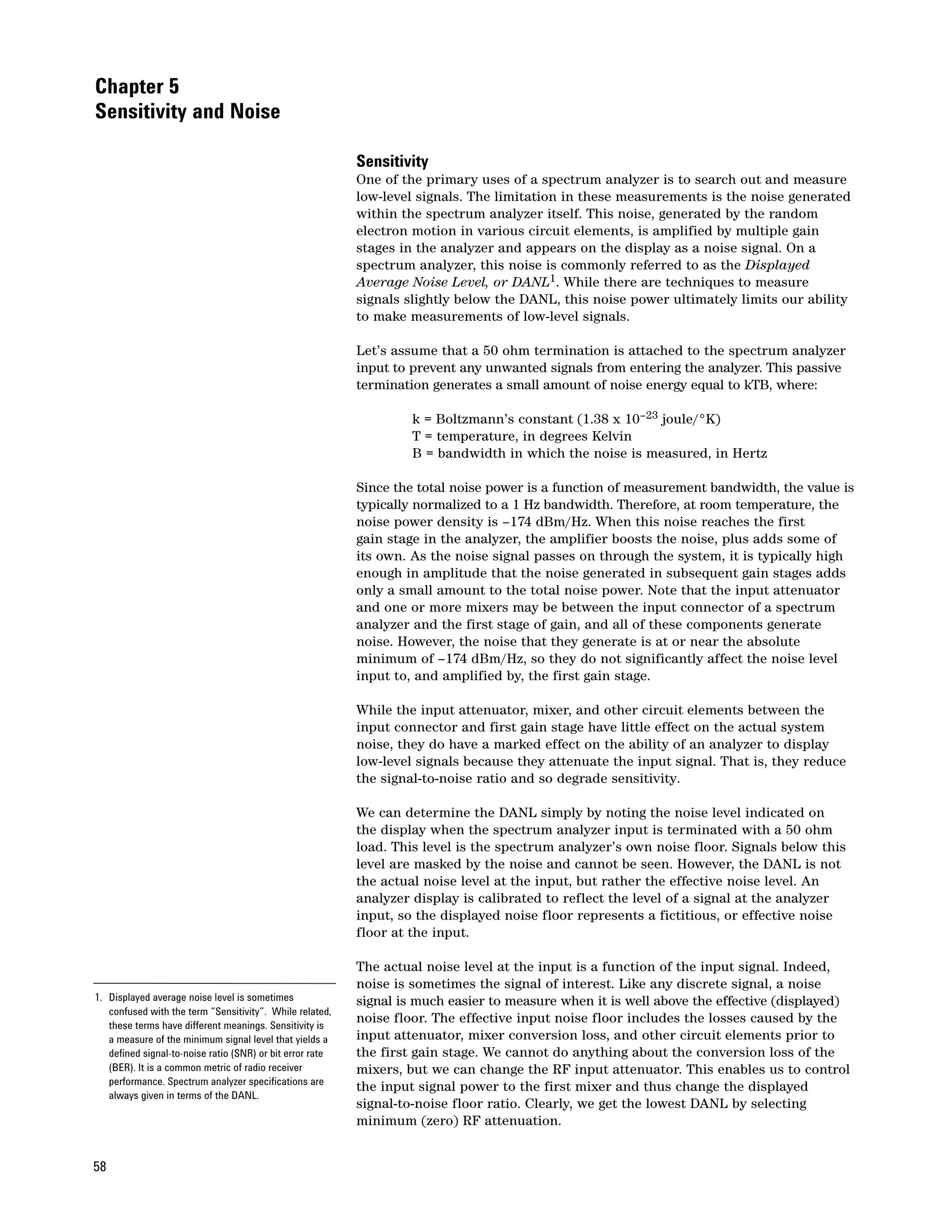
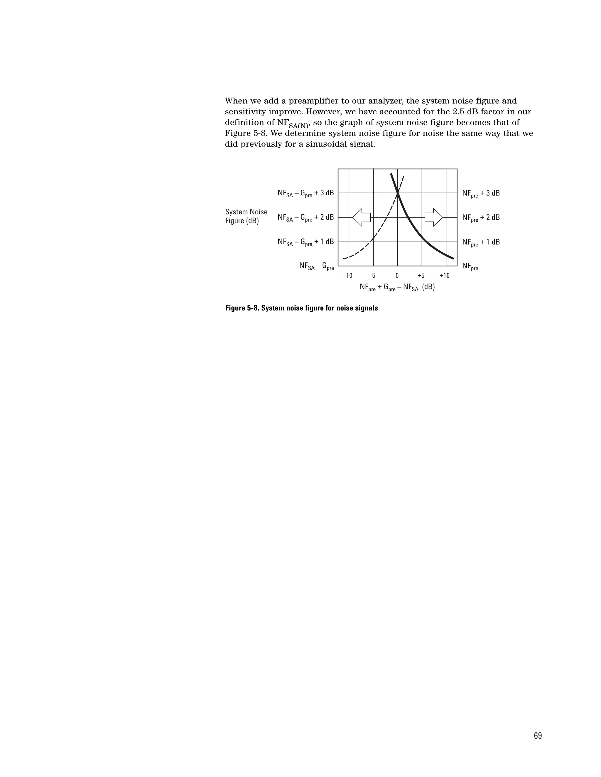
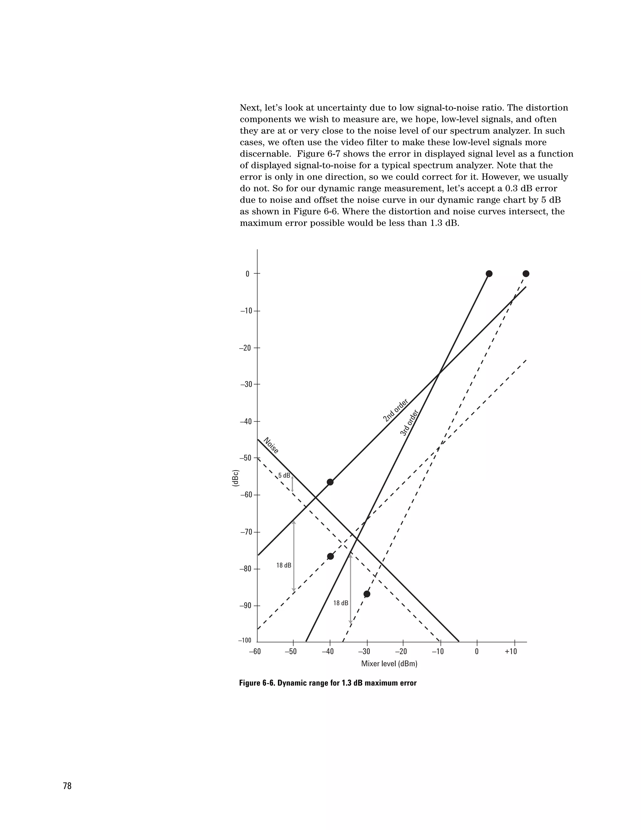
![Noise figure
Many receiver manufacturers specify the performance of their receivers in
terms of noise figure, rather than sensitivity. As we shall see, the two can
be equated. A spectrum analyzer is a receiver, and we shall examine noise
figure on the basis of a sinusoidal input.
Noise figure can be defined as the degradation of signal-to-noise ratio as a
signal passes through a device, a spectrum analyzer in our case. We can
express noise figure as:
Si/Ni
F=
So/No
where F= noise figure as power ratio (also known as noise factor)
Si = input signal power
Ni = true input noise power
So = output signal power
No = output noise power
If we examine this expression, we can simplify it for our spectrum analyzer.
First of all, the output signal is the input signal times the gain of the analyzer.
Second, the gain of our analyzer is unity because the signal level at the
output (indicated on the display) is the same as the level at the input
(input connector). So our expression, after substitution, cancellation,
and rearrangement, becomes:
F = No/Ni
This expression tells us that all we need to do to determine the noise figure
is compare the noise level as read on the display to the true (not the effective)
noise level at the input connector. Noise figure is usually expressed in terms
of dB, or:
NF = 10 log(F) = 10 log(No) – 10 log(Ni).
We use the true noise level at the input, rather than the effective noise level,
because our input signal-to-noise ratio was based on the true noise. As we
saw earlier, when the input is terminated in 50 ohms, the kTB noise level at
room temperature in a 1 Hz bandwidth is –174 dBm.
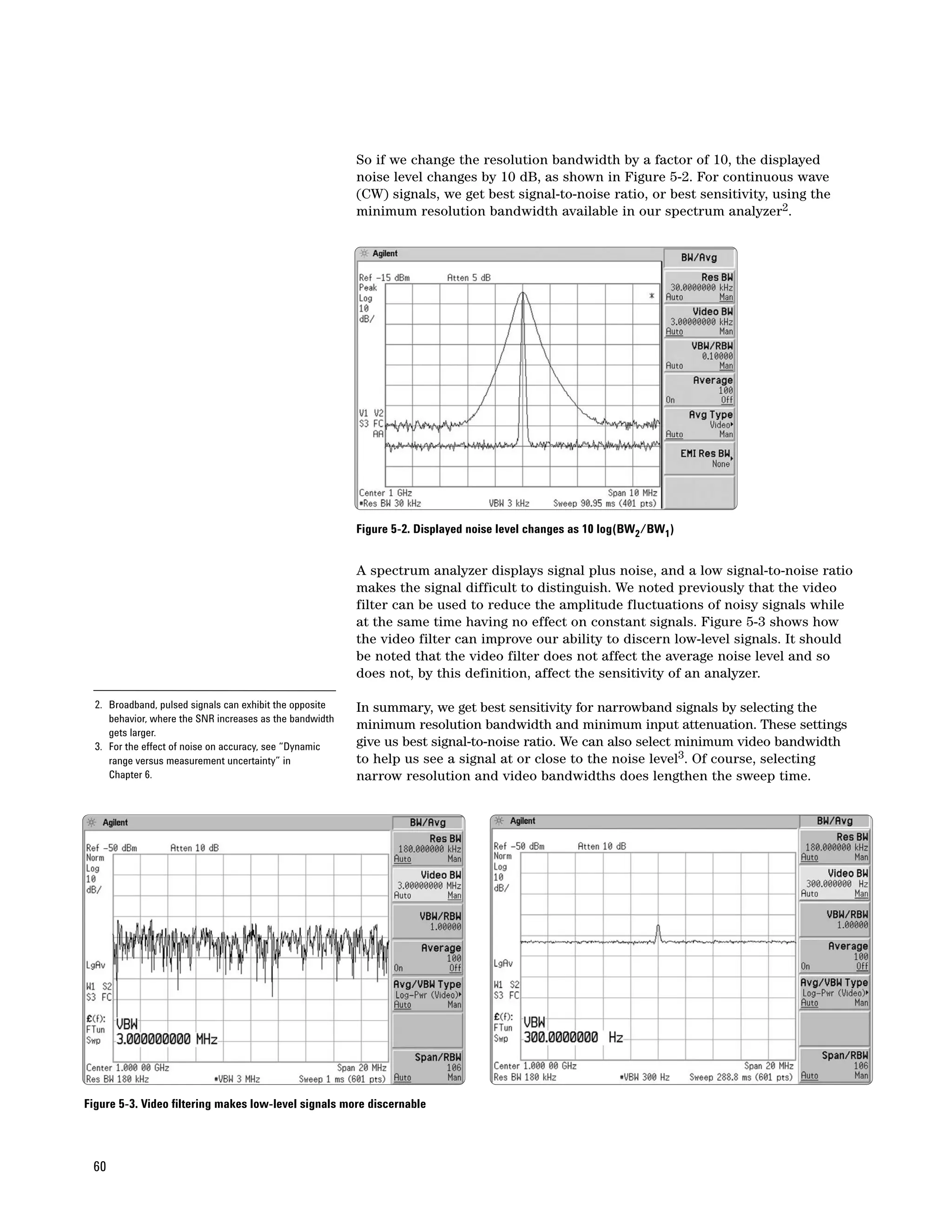
We know that the displayed level of noise on the analyzer changes with
bandwidth. So all we need to do to determine the noise figure of our
spectrum analyzer is to measure the noise power in some bandwidth,
calculate the noise power that we would have measured in a 1 Hz bandwidth
using 10 log(BW2/BW1), and compare that to –174 dBm.
For example, if we measured –110 dBm in a 10 kHz resolution bandwidth,
we would get:
NF = [measured noise in dBm] – 10 log(RBW/1) – kTBB=1 Hz
–110 dBm –10 log(10,000/1) – (–174 dBm)
–110 – 40 + 174
24 dB
4. This may not always be precisely true for a given Noise figure is independent of bandwidth4. Had we selected a different
analyzer because of the way resolution bandwidth resolution bandwidth, our results would have been exactly the same.
filter sections and gain are distributed in the IF chain.
For example, had we chosen a 1 kHz resolution bandwidth, the measured
noise would have been –120 dBm and 10 log(RBW/1) would have been 30.
Combining all terms would have given –120 – 30 + 174 = 24 dB, the same
noise figure as above.
61](https://image.slidesharecdn.com/2259filespectrumanalysisbasicsapplicationnote150aligent2005-120408110648-phpapp02/75/2259-file-spectrum_analysis_basics_application_note_150_aligent_2005-61-2048.jpg)
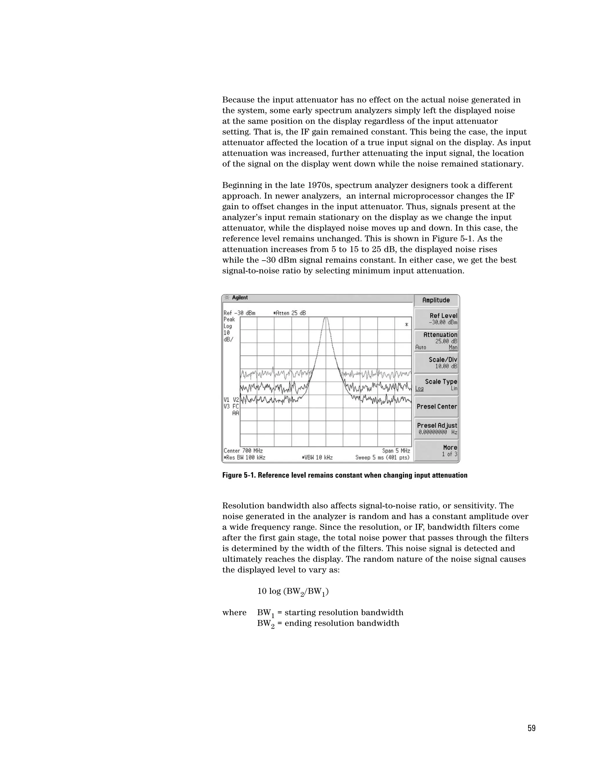
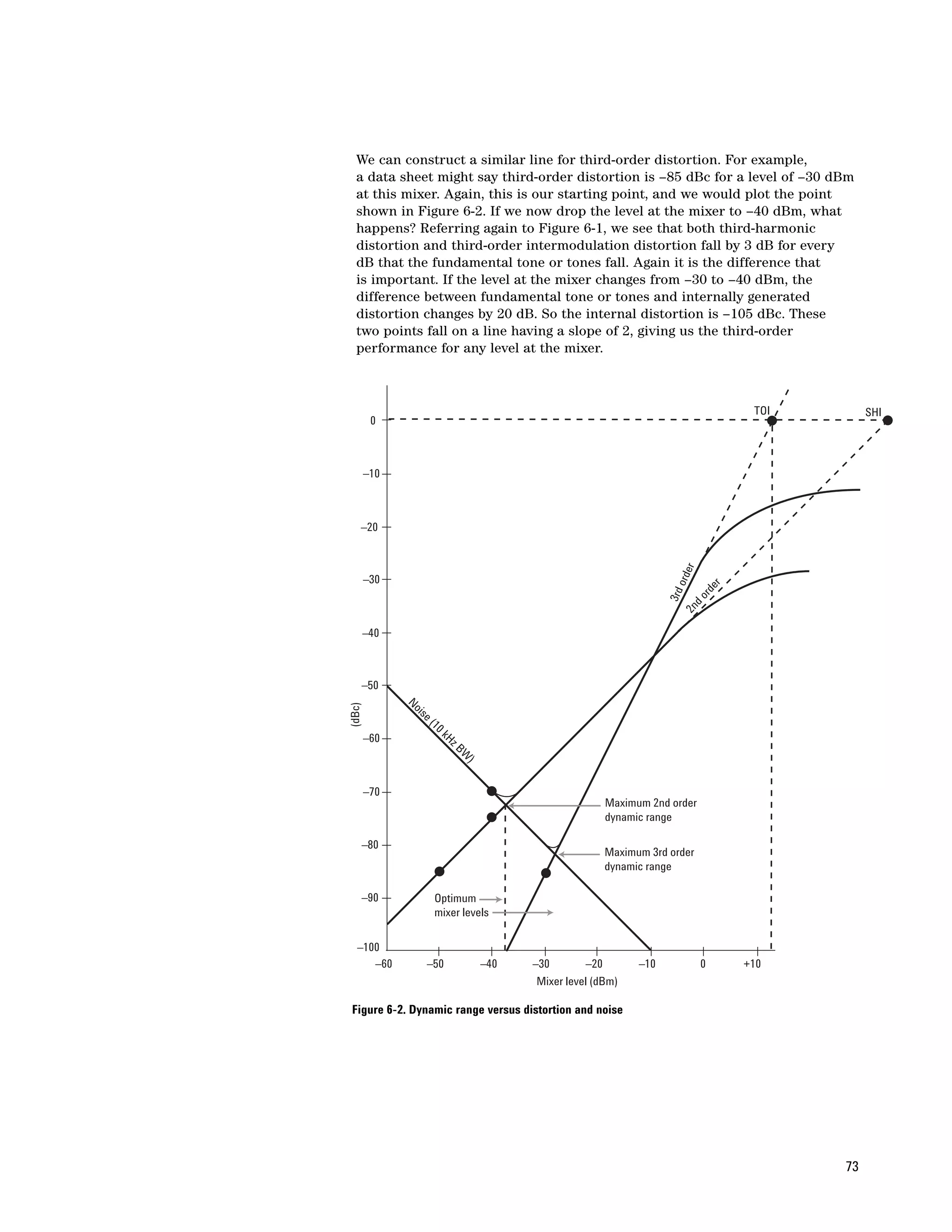
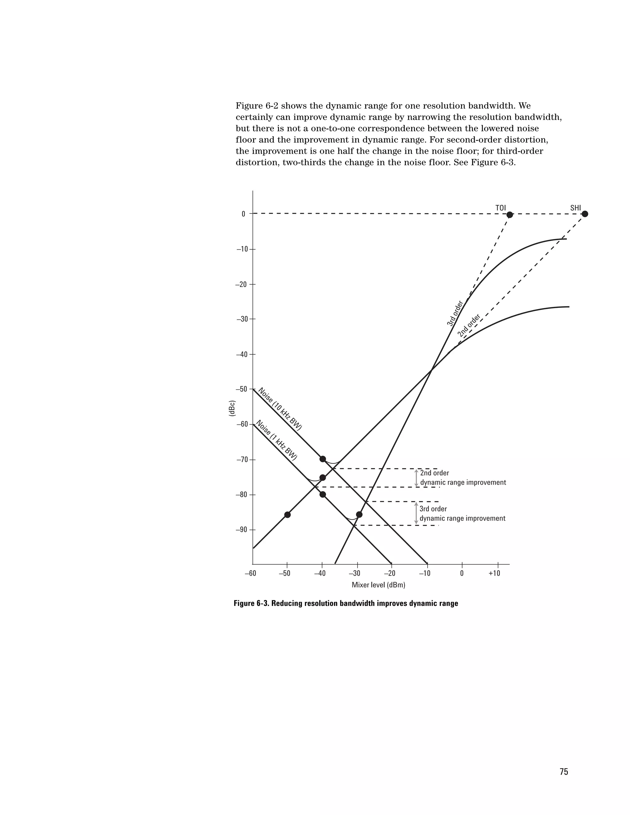
![Chapter 6
Dynamic Range
Definition
Dynamic range is generally thought of as the ability of an analyzer to measure
harmonically related signals and the interaction of two or more signals; for
example, to measure second- or third-harmonic distortion or third-order
intermodulation. In dealing with such measurements, remember that the
input mixer of a spectrum analyzer is a non-linear device, so it always
generates distortion of its own. The mixer is non-linear for a reason. It must
be nonlinear to translate an input signal to the desired IF. But the unwanted
distortion products generated in the mixer fall at the same frequencies as
the distortion products we wish to measure on the input signal.
So we might define dynamic range in this way: it is the ratio, expressed in dB,
of the largest to the smallest signals simultaneously present at the input of
the spectrum analyzer that allows measurement of the smaller signal to a
given degree of uncertainty.
Notice that accuracy of the measurement is part of the definition. We shall
see how both internally generated noise and distortion affect accuracy in the
following examples.
Dynamic range versus internal distortion
To determine dynamic range versus distortion, we must first determine just
how our input mixer behaves. Most analyzers, particularly those utilizing
harmonic mixing to extend their tuning range1, use diode mixers. (Other
types of mixers would behave similarly.) The current through an ideal diode
can be expressed as:
i = Is(eqv/kT–1)
where IS = the diode’s saturation current
q = electron charge (1.60 x 10⁻¹⁹ C)
v = instantaneous voltage
k = Boltzmann’s constant (1.38 x 10⁻²³ joule/°K)
T= temperature in degrees Kelvin
We can expand this expression into a power series:
i = Is(k1v + k2v2 + k3v3 +...)
where k1 = q/kT
k2 = k12/2!
k3 = k13/3!, etc.
Let’s now apply two signals to the mixer. One will be the input signal that
we wish to analyze; the other, the local oscillator signal necessary to create
the IF:
v = VLO sin(ωLOt) + V1 sin(ω1t)
If we go through the mathematics, we arrive at the desired mixing product
that, with the correct LO frequency, equals the IF:
k2VLOV1 cos[(ωLO – ω1)t]
A k2VLOV1 cos[(ωLO + ω1)t] term is also generated, but in our discussion
of the tuning equation, we found that we want the LO to be above the IF, so
1. See Chapter 7, “Extending the Frequency Range.” (ωLO + ω1) is also always above the IF.
70](https://image.slidesharecdn.com/2259filespectrumanalysisbasicsapplicationnote150aligent2005-120408110648-phpapp02/75/2259-file-spectrum_analysis_basics_application_note_150_aligent_2005-70-2048.jpg)
![With a constant LO level, the mixer output is linearly related to the input
signal level. For all practical purposes, this is true as long as the input signal
is more than 15 to 20 dB below the level of the LO. There are also terms
involving harmonics of the input signal:
(3k3/4)VLOV12 sin(ωLO – 2 ω1)t,
(k4 /8)VLOV13 sin(ωLO – 3ω1)t, etc.
These terms tell us that dynamic range due to internal distortion is a
function of the input signal level at the input mixer. Let’s see how this works,
using as our definition of dynamic range, the difference in dB between the
fundamental tone and the internally generated distortion.
The argument of the sine in the first term includes 2ω1, so it represents
the second harmonic of the input signal. The level of this second harmonic
is a function of the square of the voltage of the fundamental, V12. This fact
tells us that for every dB that we drop the level of the fundamental at the
input mixer, the internally generated second harmonic drops by 2 dB.
See Figure 6-1. The second term includes 3ω1, the third harmonic, and the
cube of the input-signal voltage, V13. So a 1 dB change in the fundamental
at the input mixer changes the internally generated third harmonic by 3 dB.
Distortion is often described by its order. The order can be determined by
noting the coefficient associated with the signal frequency or the exponent
associated with the signal amplitude. Thus second-harmonic distortion is
second order and third harmonic distortion is third order. The order also
indicates the change in internally generated distortion relative to the change
in the fundamental tone that created it.
Now let us add a second input signal:
v = VLO sin(ωLO t) + V1 sin(ω1t) + V2 sin(ω2t)
This time when we go through the math to find internally generated distortion,
in addition to harmonic distortion, we get:
(k4/8)VLOV12V2 cos[ωLO – (2 ω1 – ω2)]t,
(k4/8)VLOV1V22 cos[ωLO – (2 ω2 – ω1)]t, etc.
D dB D dB D dB
2D dB
3D dB
3D dB 3D dB
w 2w 3w 2w1 – w2 w1 w2 2w2 – w1
Figure 6-1. Changing the level of fundamental tones at the mixer
71](https://image.slidesharecdn.com/2259filespectrumanalysisbasicsapplicationnote150aligent2005-120408110648-phpapp02/75/2259-file-spectrum_analysis_basics_application_note_150_aligent_2005-71-2048.jpg)
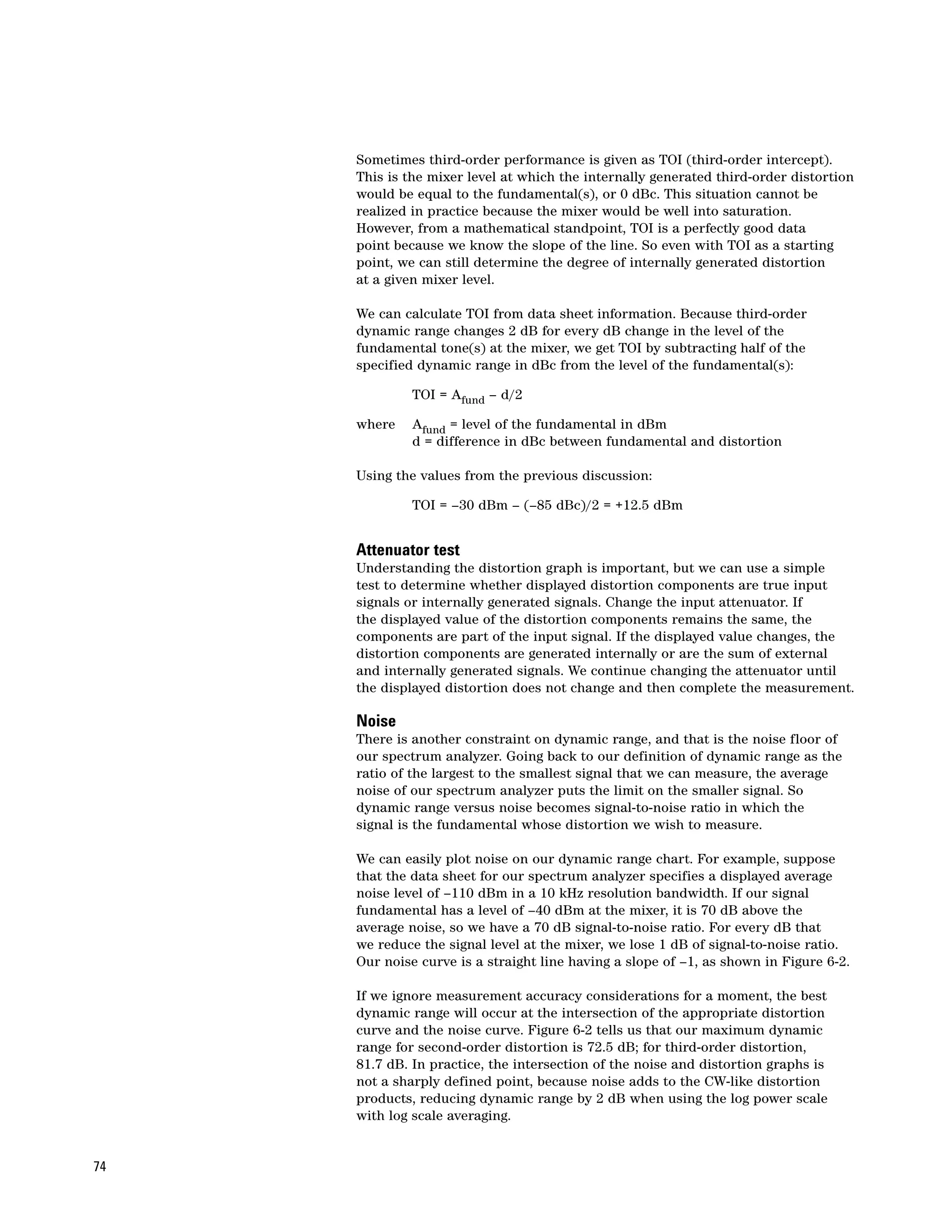
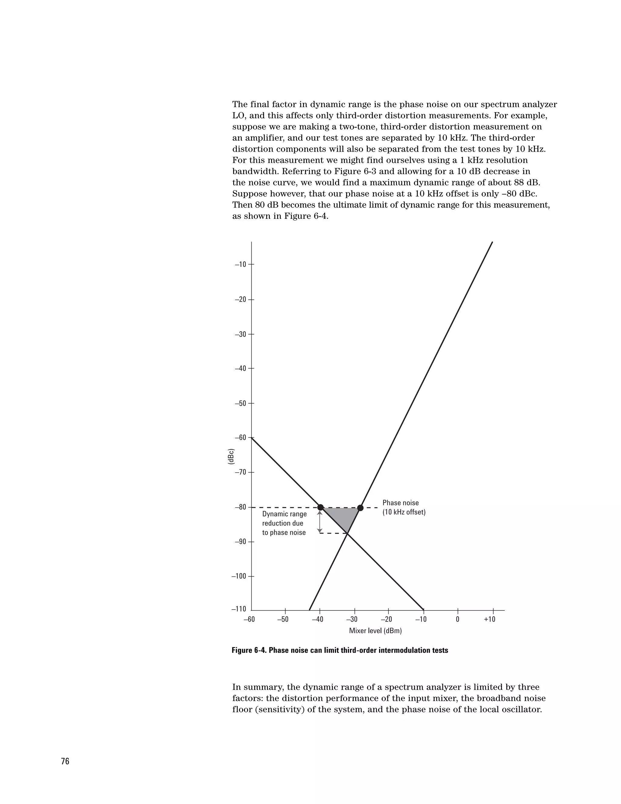

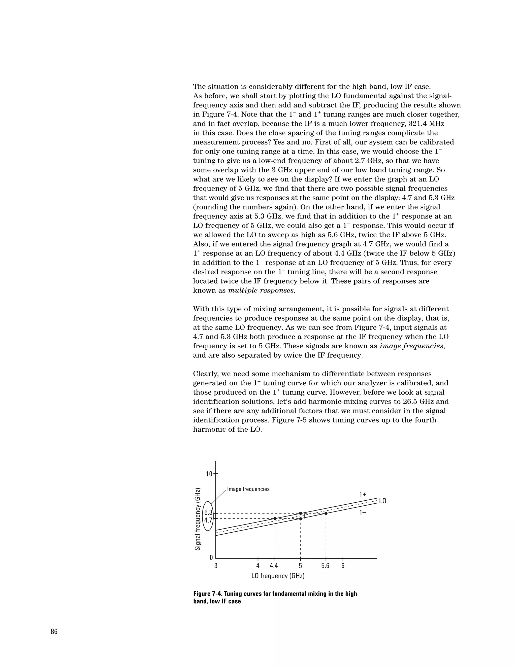
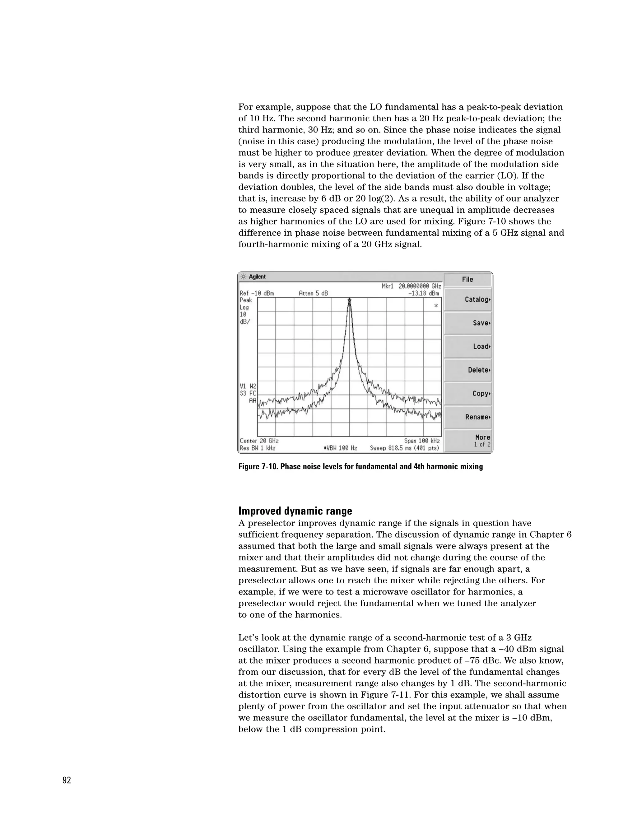
![From the graph, we see that a –10 dBm signal at the mixer produces a
second-harmonic distortion component of –45 dBc. Now we tune the analyzer
to the 6 GHz second harmonic. If the preselector has 70 dB rejection, the
fundamental at the mixer has dropped to –80 dBm. Figure 7-11 indicates
that for a signal of –80 dBm at the mixer, the internally generated distortion
is –115 dBc, meaning 115 dB below the new fundamental level of –80 dBm.
This puts the absolute level of the harmonic at –195 dBm. So the difference
between the fundamental we tuned to and the internally generated second
harmonic we tuned to is 185 dB! Clearly, for harmonic distortion, dynamic
range is limited on the low-level (harmonic) end only by the noise floor
(sensitivity) of the analyzer.
–45
–50
–60
Internal distortion (dBc)
–70
–80
–90
–100
–110
–115
–120
–90 –80 –70 –60 –50 –40 –30 –20 –10 0
Mixed level (dBm)
Figure 7-11. Second-order distortion graph
What about the upper, high-level end? When measuring the oscillator
fundamental, we must limit power at the mixer to get an accurate reading
of the level. We can use either internal or external attenuation to limit
the level of the fundamental at the mixer to something less than the 1 dB
compression point. However, since the preselector highly attenuates the
fundamental when we are tuned to the second harmonic, we can remove
some attenuation if we need better sensitivity to measure the harmonic.
A fundamental level of +20 dBm at the preselector should not affect our
ability to measure the harmonic.
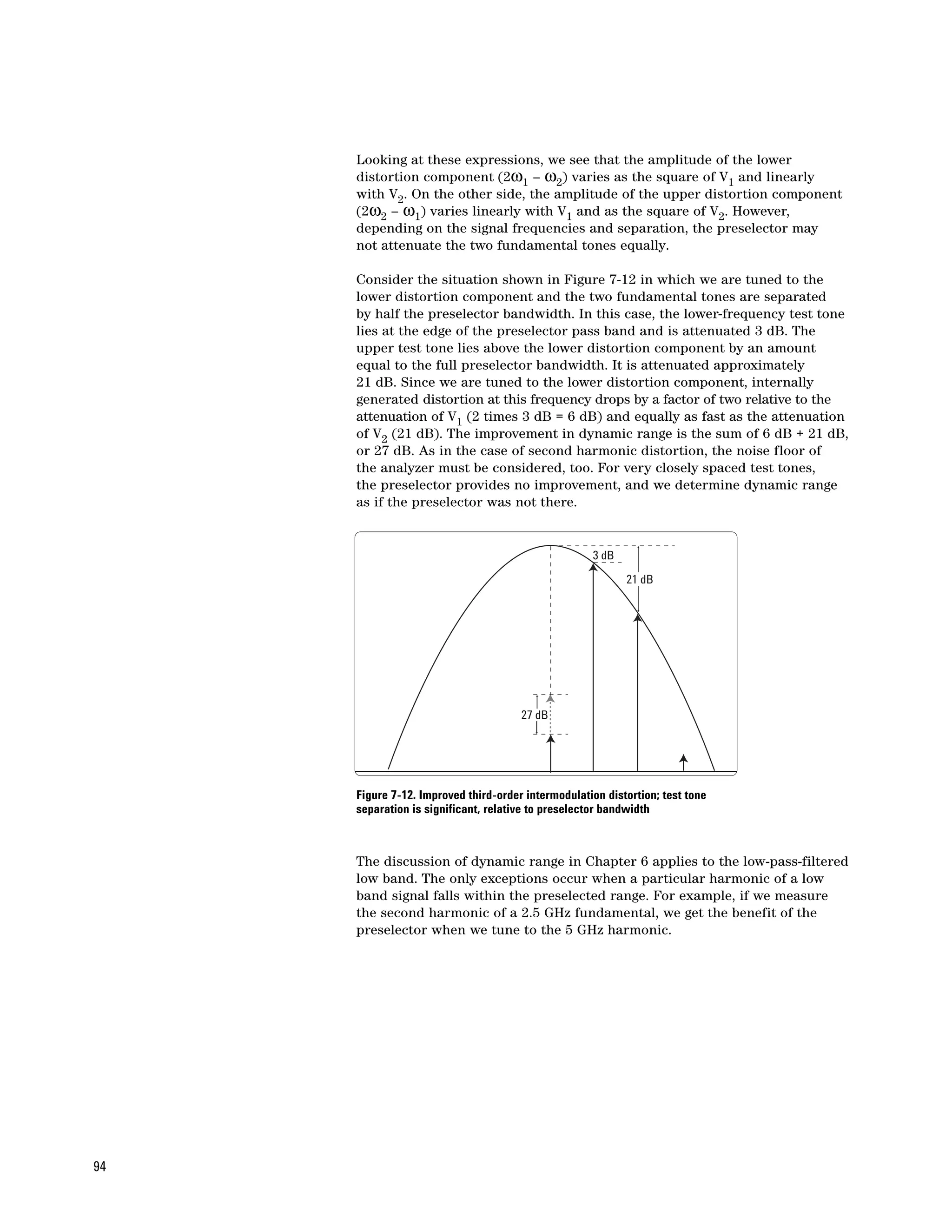
Any improvement in dynamic range for third-order intermodulation
measurements depends upon separation of the test tones versus preselector
bandwidth. As we noted, typical preselector bandwidth is about 35 MHz at
the low end and 80 MHz at the high end. As a conservative figure, we might
use 18 dB per octave of bandwidth roll off of a typical YIG preselector filter
beyond the 3 dB point. So to determine the improvement in dynamic range,
we must determine to what extent each of the fundamental tones is
attenuated and how that affects internally generated distortion. From
the expressions in Chapter 6 for third-order intermodulation, we have:
(k4/8)VLOV12V2 cos[ωLO – (2ω1 – ω2)]t
and
(k4/8)VLOV1V22 cos[ωLO – (2ω2 – ω1)]t
93](https://image.slidesharecdn.com/2259filespectrumanalysisbasicsapplicationnote150aligent2005-120408110648-phpapp02/75/2259-file-spectrum_analysis_basics_application_note_150_aligent_2005-93-2048.jpg)
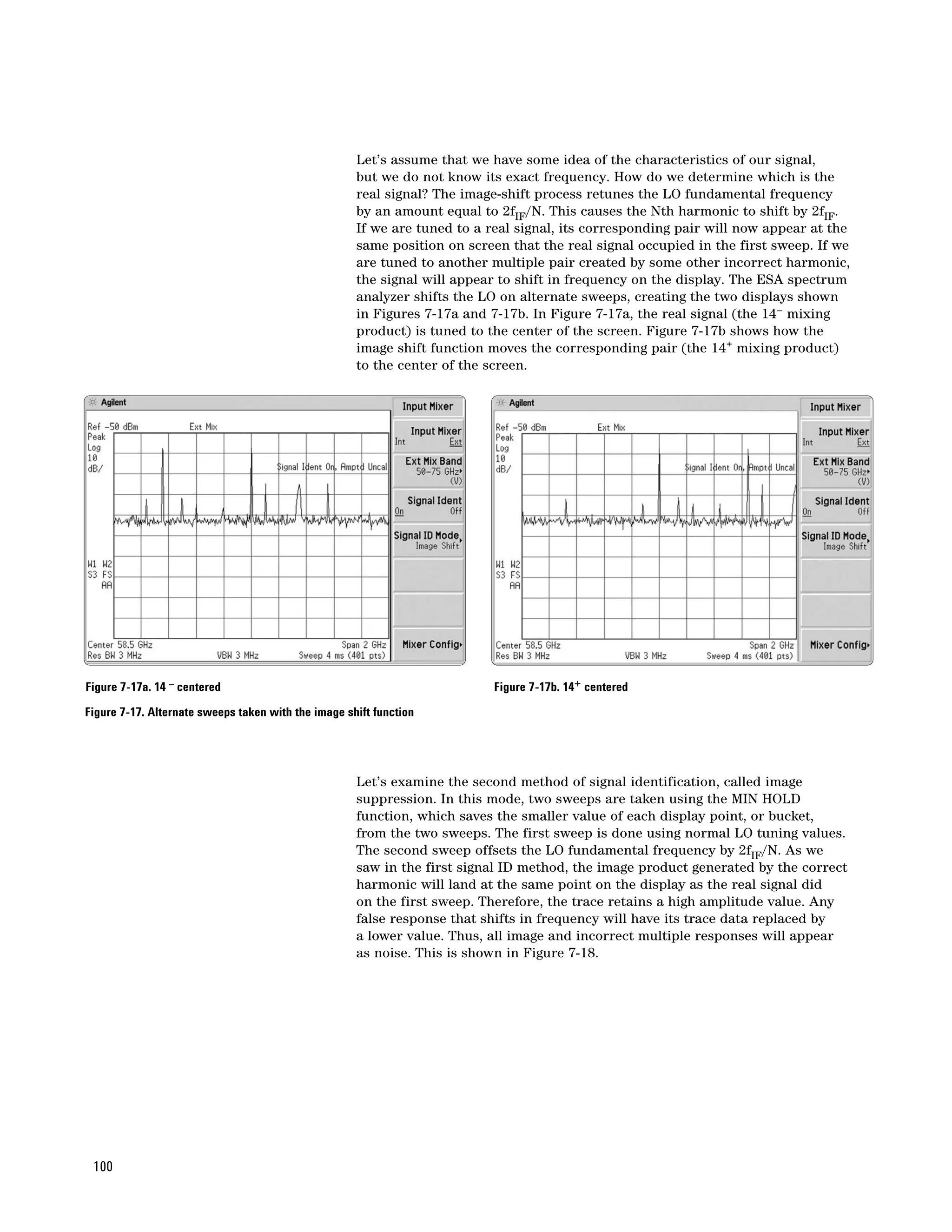
![Figure 7-18. The image suppress function displays only real signals
Note that both signal identification methods are used for identifying correct
frequencies only. You should not attempt to make amplitude measurements
while the signal identification function is turned on. Note that in both
Figures 7-17 and 7-18, an on-screen message alerts the user to this fact.
Once we have identified the real signal of interest, we turn off the signal
ID function and zoom in on it by reducing the span. We can then measure
the signal’s amplitude and frequency. See Figure 7-19.
To make an accurate amplitude measurement, it is very important that you
first enter the calibration data for your external mixer. This data is normally
supplied by the mixer manufacturer, and is typically a table of mixer conversion
loss, in dB, at a number of frequency points across the band. This data is
entered into the ESA’s amplitude correction table. This table is accessed by
pressing the [AMPLITUDE] key, then pressing the {More}, {Corrections},
{Other} and {Edit} softkeys. After entering the conversion loss values, apply
the corrections with the {Correction On} softkey. The spectrum analyzer
reference level is now calibrated for signals at the input to the external mixer.
If you have other loss or gain elements between the signal source and the
mixer, such as antennas, cables, or preamplifiers, the frequency responses of
these elements should be entered into the amplitude correction table as well.
Figure 7-19. Measurement of positively identified signal
101](https://image.slidesharecdn.com/2259filespectrumanalysisbasicsapplicationnote150aligent2005-120408110648-phpapp02/75/2259-file-spectrum_analysis_basics_application_note_150_aligent_2005-101-2048.jpg)
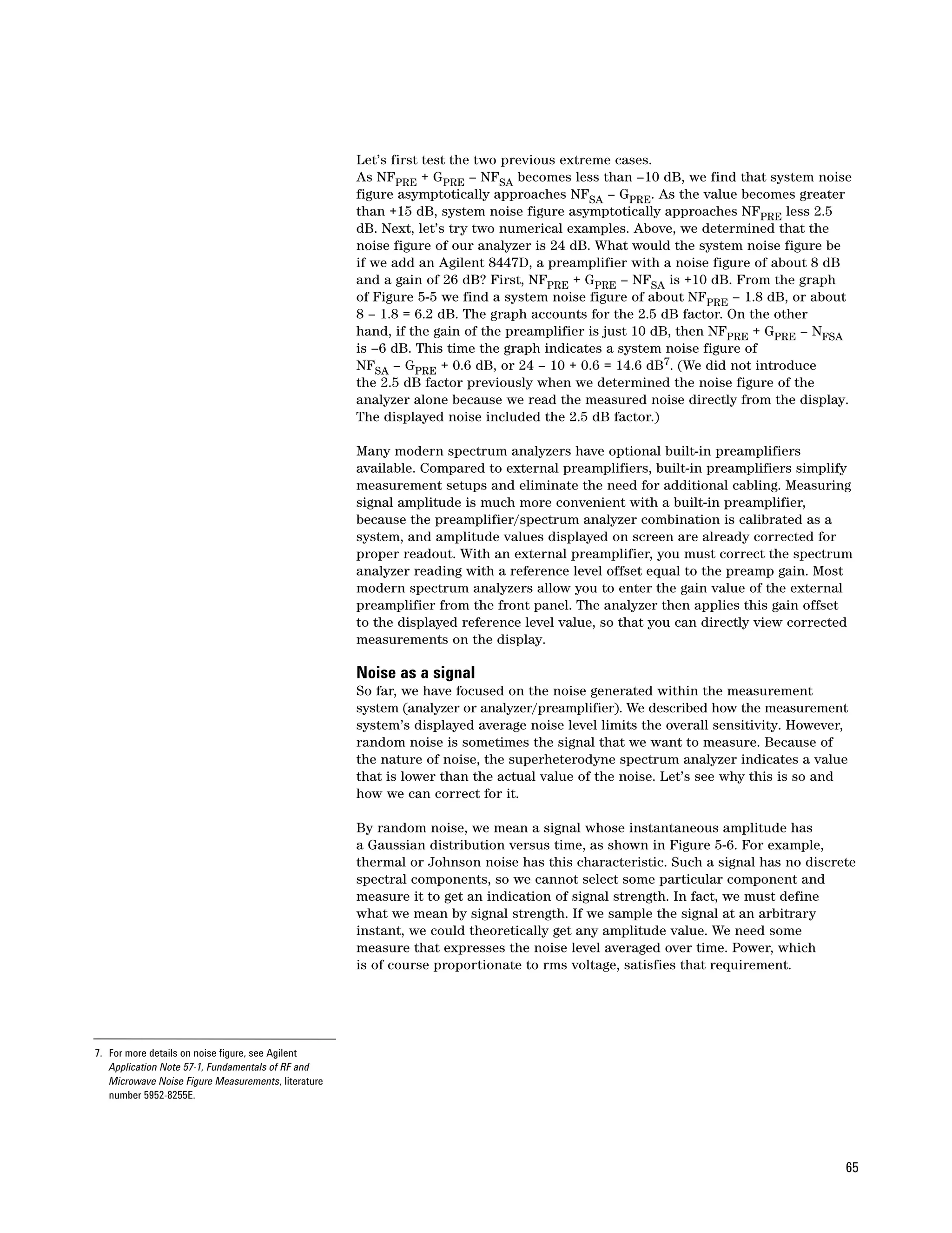
![Video: In a spectrum analyzer, a term describing the output of the envelope
detector. The frequency range extends from 0 Hz to a frequency typically
well beyond the widest resolution bandwidth available in the analyzer.
However, the ultimate bandwidth of the video chain is determined by the
setting of the video filter.
Video amplifier: A post-detection, DC-coupled amplifier that drives the
vertical deflection plates of the CRT. See Video bandwidth and Video filter.
Video average: A digital averaging of a spectrum analyzer’s trace
information. The averaging is done at each point of the display independently
and is completed over the number of sweeps selected by the user. The
averaging algorithm applies a weighting factor (1/n, where n is the number
of the current sweep) to the amplitude value of a given point on the current
sweep, applies another weighting factor [(n – 1)/n] to the previously
stored average, and combines the two for a current average. After the
designated number of sweeps are completed, the weighting factors remain
constant, and the display becomes a running average.
Video bandwidth: The cutoff frequency (3 dB point) of an adjustable low
pass filter in the video circuit. When the video bandwidth is equal to or less
than the resolution bandwidth, the video circuit cannot fully respond to
the more rapid fluctuations of the output of the envelope detector. The
result is a smoothing of the trace, i.e. a reduction in the peak-to-peak
excursion of broadband signals such as noise and pulsed RF when viewed
in the broadband mode. The degree of averaging or smoothing is a function
of the ratio of the video bandwidth to the resolution bandwidth.
Video filter: A post-detection, low-pass filter that determines the
bandwidth of the video amplifier. Used to average or smooth a trace.
See Video bandwidth.
Zero span: That case in which a spectrum analyzer’s LO remains fixed
at a given frequency so the analyzer becomes a fixed-tuned receiver. The
bandwidth of the receiver is that of the resolution (IF) bandwidth. Signal
amplitude variations are displayed as a function of time. To avoid any loss
of signal information, the resolution bandwidth must be as wide as the
signal bandwidth. To avoid any smoothing, the video bandwidth must be
set wider than the resolution bandwidth.
119](https://image.slidesharecdn.com/2259filespectrumanalysisbasicsapplicationnote150aligent2005-120408110648-phpapp02/75/2259-file-spectrum_analysis_basics_application_note_150_aligent_2005-119-2048.jpg)

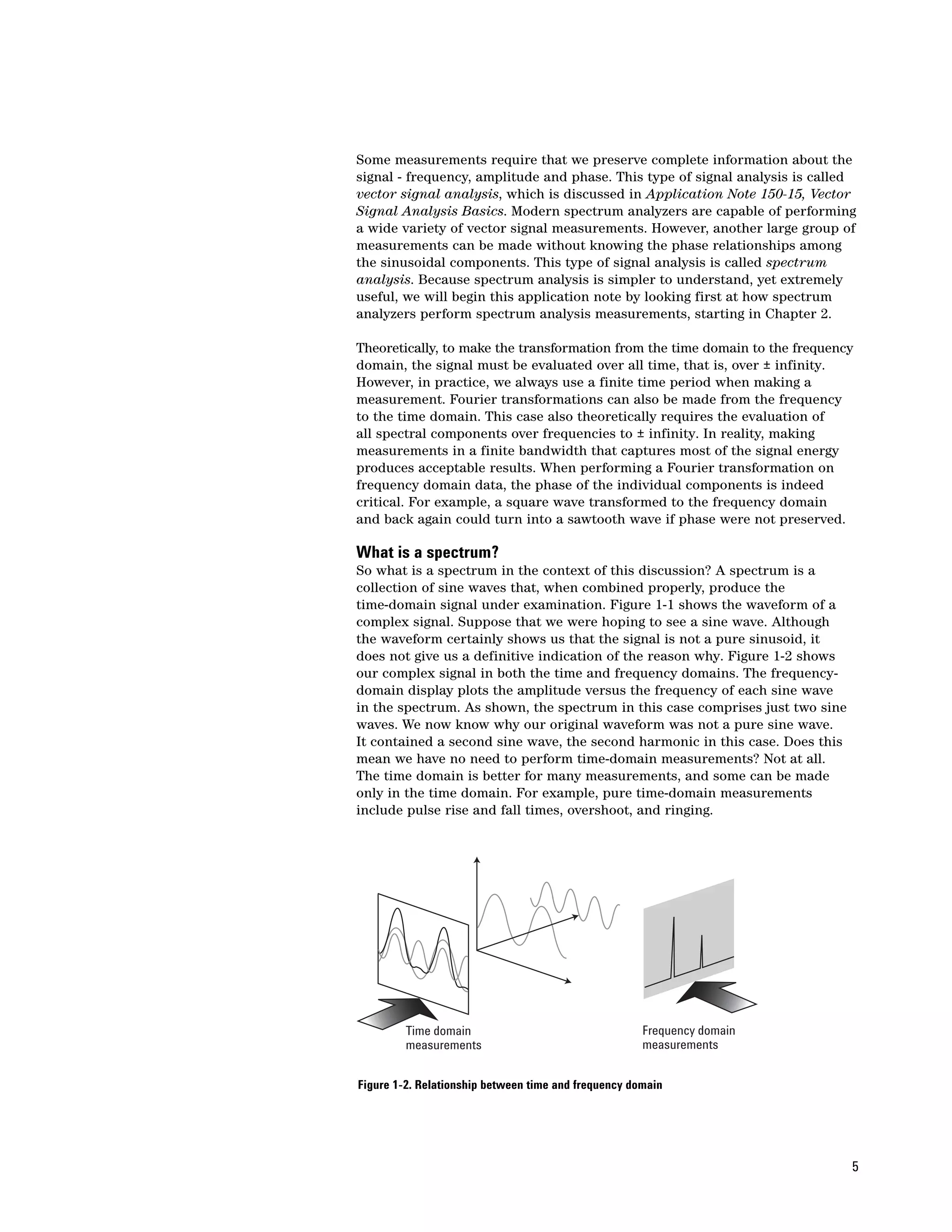
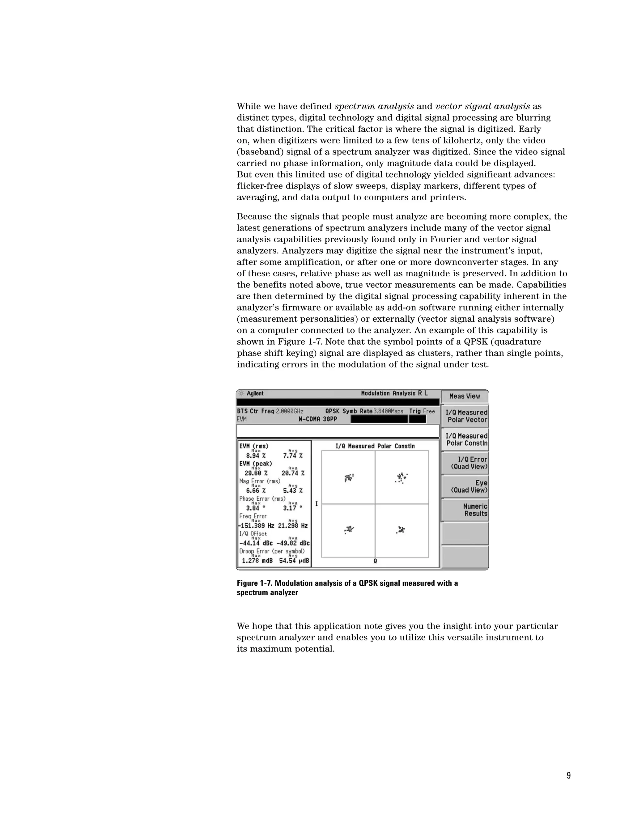
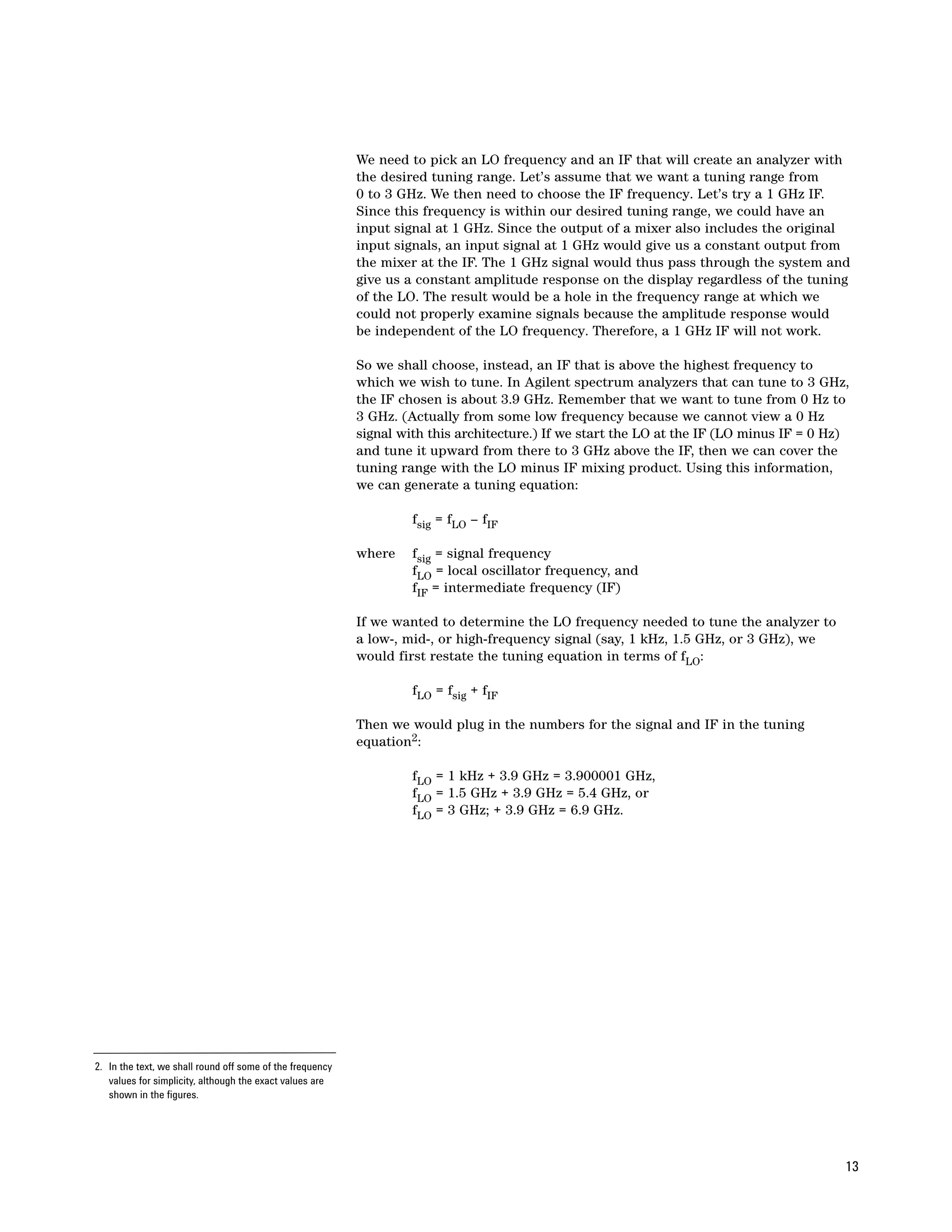
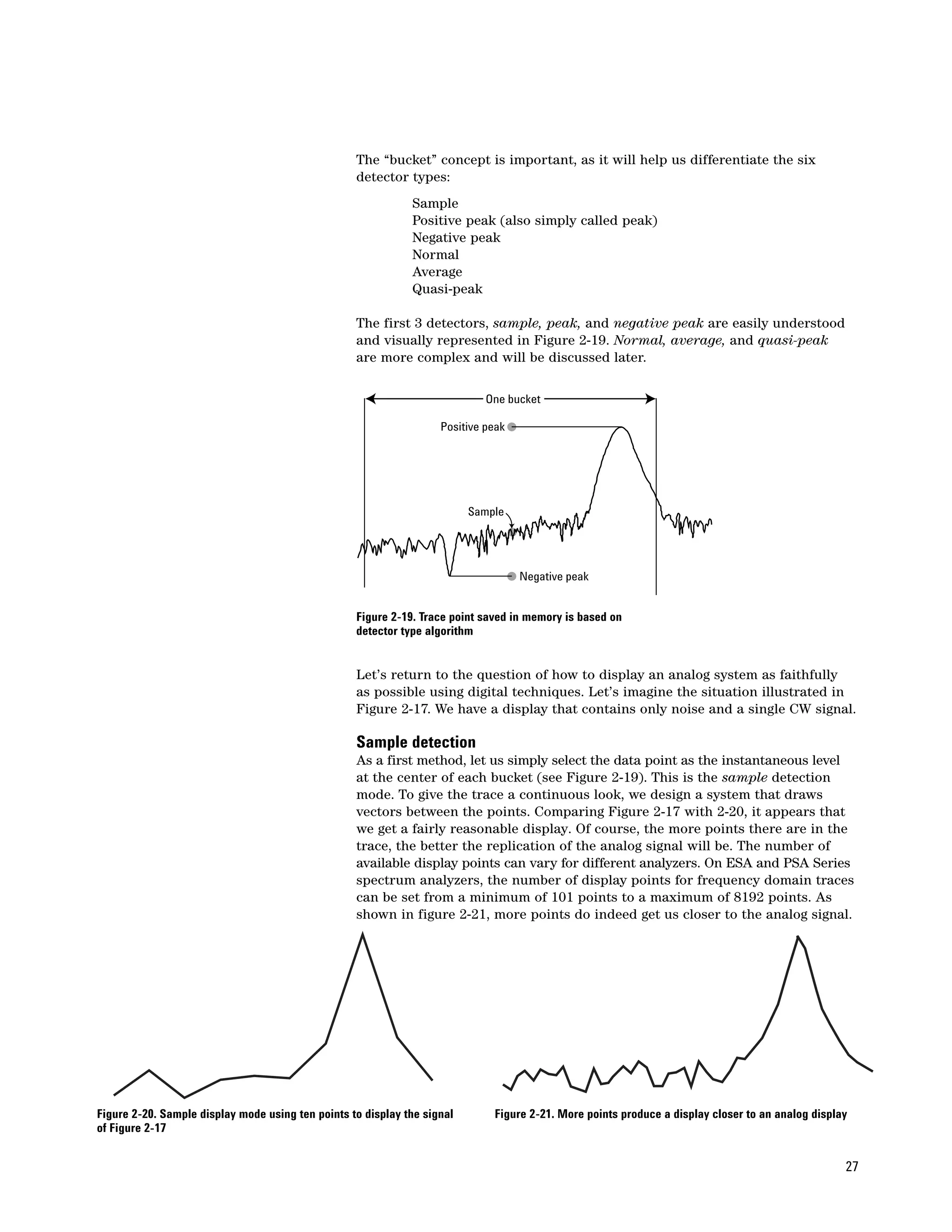
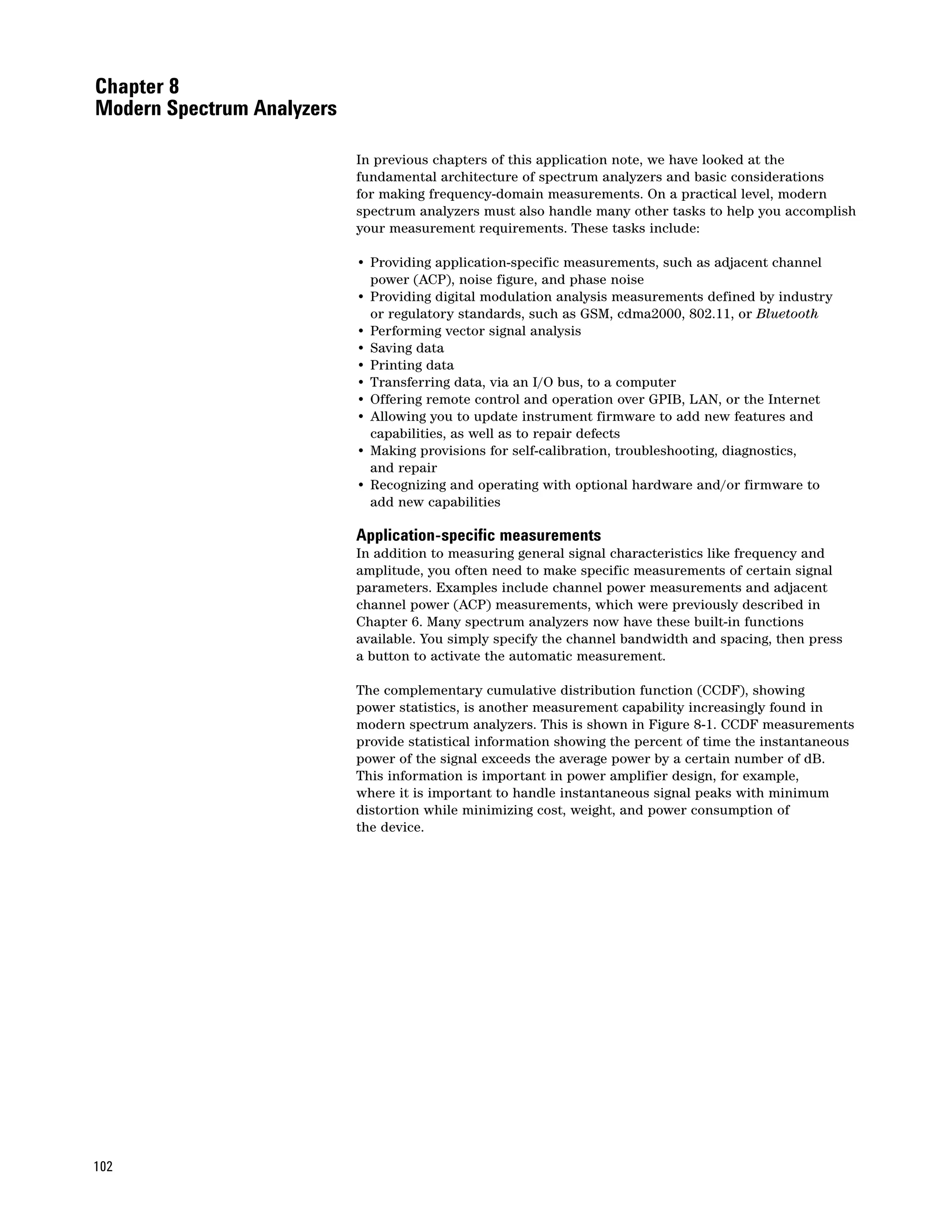
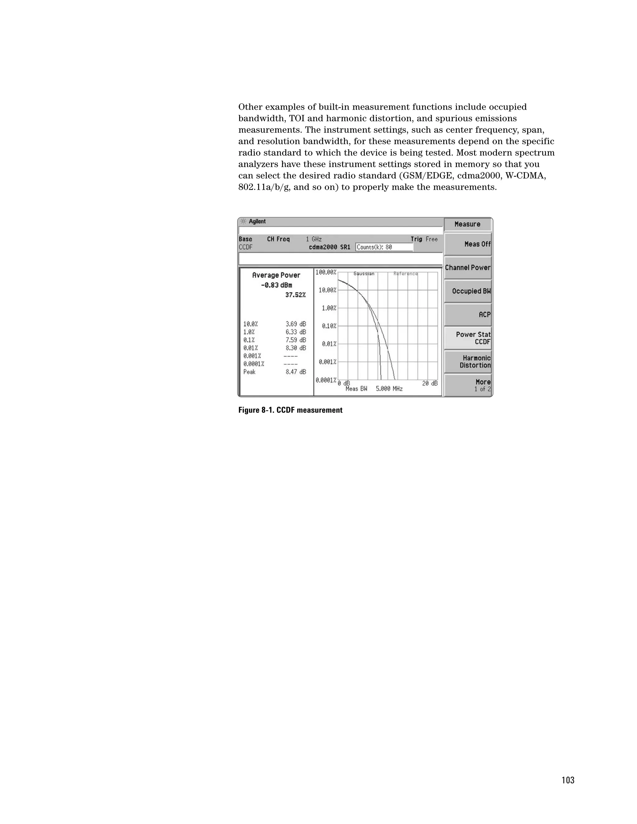
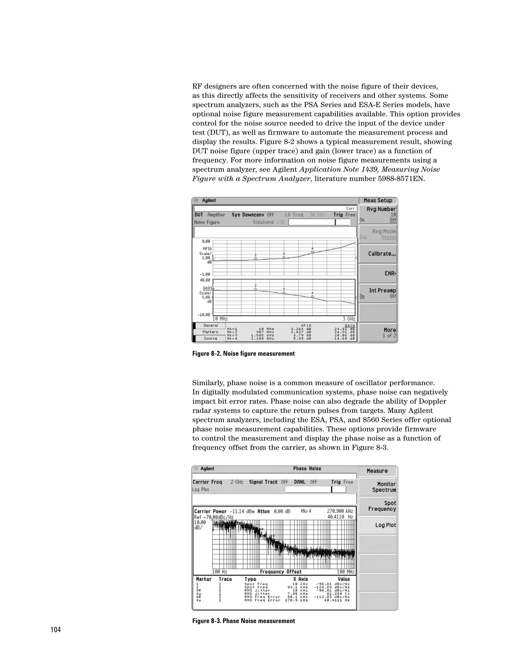
This document provides an overview of spectrum analysis and spectrum analyzer fundamentals. It discusses topics such as the frequency domain versus time domain, why spectra are measured, types of measurements and signal analyzers. It also covers the basic components and functioning of spectrum analyzers, including RF attenuators, filters, tuning, detectors, displays and more. Modern developments like digital IF and application-specific measurements are also summarized.


![Coded Agents – with UiPath SDK + LangGraph [Virtual Hands-on Workshop]](https://cdn.slidesharecdn.com/ss_thumbnails/codedagentsdeck-251215155422-5497c599-thumbnail.jpg?width=640&height=640&fit=bounds)


