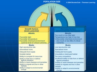
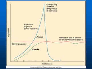
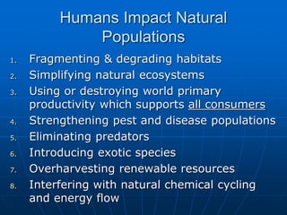
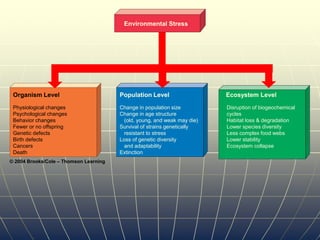
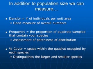
The document details concepts related to populations, including definitions, dynamics, and measurement techniques such as the Lincoln index and quadrat method. It explores factors influencing population growth, such as biotic potential and environmental resistance, and distinguishes between r-strategist and k-strategist species, as well as their reproductive patterns. Additionally, it addresses human impacts on natural populations and emphasizes the importance of monitoring changes in populations over time.

1. Populations, Their changes
and Their measurement
IB syllabus: 2.1, 2.5
AP syllabus
Ch 9

2. 2.1 Species and Populations
 A population is a group of organisms of the same species living
in the same area at the same time, and which are capable of
interbreeding.
 • S and J population curves describe a generalized response of
populations to a particular set of conditions (abiotic and biotic
factors).
 • Limiting factors will slow population growth as it approaches
the carrying capacity of the system
 Organisms in an ecosystem can be identified using a variety of
tools including keys, comparison to herbarium or specimen
collections, technologies and scientific expertise
 Methods for estimating the abundance of non-motile organisms
include the usecof quadrats for making actual counts, measuring
population density, percentage cover and percentage frequency.

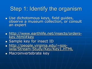
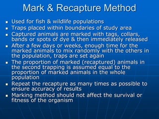
3.  Direct and indirect methods for estimating the abundance of
motile organisms can be described and evaluated. Direct
methods include actual counts and sampling. Indirect methods
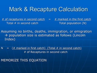
include the use of capture–mark–recapture with the application
of the Lincoln index.
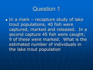
 Lincoln Index = [(n1) (n2)] / nm
 – n1 is the number caught in the first sample
 – n2 is the number caught in the second sample
 – nm is the number caught in the second sample that were
marked
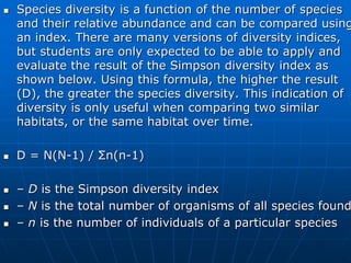
 Species richness is the number of species in a community and is
a useful comparative measure.

4.  Species diversity is a function of the number of species
and their relative abundance and can be compared using
an index. There are many versions of diversity indices,
but students are only expected to be able to apply and
evaluate the result of the Simpson diversity index as
shown below. Using this formula, the higher the result
(D), the greater the species diversity. This indication of
diversity is only useful when comparing two similar
habitats, or the same habitat over time.
 D = N(N-1) / Σn(n-1)
 – D is the Simpson diversity index
 – N is the total number of organisms of all species found
 – n is the number of individuals of a particular species

5. Vocabulary
 Abiotic factor
 Biotic factor
 Carrying Capacity
 Habitat
 K-strategist
 Population
 r-strategist

6. OTTERS & KELP FORESTS
http://www.youtube.com/watch?v=eYpM-
qDNKzs&safe=active

7. Population
 A group of individuals of the same
species found in the same area
(habitat) at the same time
 The gopher tortoises in scrub
habitats in Volusia county
 The bottlenose dolphins of the Indian
River Lagoon

8. Sea Otters: A case study
 Sea otters keystone species in Pacific kelp forests
 Daily consume 25% body weight in urchins &
molluscs
 Population > 1 million before settlers arrived
 1700’s hunted to near extinction – 1000 in the
Aleutians, AK only 20 off California
 In 1971 A-bomb test in AK used sea otter
population to assess bomb’s power  1000’s died
 1973 Endangered Species Act passes, 1976
Marine Mammal Conservation Act
 1989 1000’s died in Exxon Valdez Oil spill
 Otters recovering in most places after 1970’s
 The spring 2008 survey found 2760 sea otters,
down 8.8-percent from the record 2007 spring
survey.

9. New Threats?
Pollution Effects
- Shellfish magnify
toxins
- Reduce disease
resistance
- Reduce fertility
Increased Predation
- Killer Whales
- Switch to otters
when other food
is scarce

10. Population characteristics
 Populations are dynamic – change in
response to environment
• Size (# of individuals)
• Density (# of individuals in a certain space)
• Dispersion (spatial pattern of individuals)
 Random, Uniform, Clumped  based on food
• Age distribution (proportion of each age)
 Changes called Population dynamics
• Respond to environmental stress & change

11. Clumped
(elephants)
Uniform
(creosote bush)
Random
(dandelions)
Common Dispersion Patterns
Clumped is most common because resources have a patchy
distribution.

12. Limiting Factors & Population
Growth
 4 variables govern changes in
population size
• Birth, Death, Immigration, emigration
 Variables are dependent on resource
availability & environmental
conditions
 Population change = (Birth +
Immigration)– (Death + Emigration)

13. POPULATION SIZE
Growth factors
(biotic potential)
Favorable light
Favorable temperature
Favorable chemical environment
(optimal level of critical nutrients)
Abiotic
Biotic
High reproductive rate
Generalized niche
Adequate food supply
Suitable habitat
Ability to compete for resources
Ability to hide from or defend
against predators
Ability to resist diseases and parasites
Ability to migrate and live in other
habitats
Ability to adapt to environmental
change
Decrease factors
(environmental resistance)
Too much or too little light
Temperature too high or too low
Unfavorable chemical environment
(too much or too little of critical
nutrients)
Abiotic
Biotic
Low reproductive rate
Specialized niche
Inadequate food supply
Unsuitable or destroyed habitat
Too many competitors
Insufficient ability to hide from or defend
against predators
Inability to resist diseases and parasites
Inability to migrate and live in other
habitats
Inability to adapt to environmental
change
© 2004 Brooks/Cole – Thomson Learning

14. Capacity for Growth
 Capacity for growth = Biotic potential
 Rate at which a population grows with
unlimited resources is intrinsic rate of
increase (r)
 High (r)  (1)reproduce early in life,
(2)short generation time, (3)multiple
reproductive events, (4)many offspring each
time
 BUT – no population can grow indefinitely
 Always limits on population growth in nature

15. Carrying Capacity
 Environmental resistance = all
factors which limit the growth of
populations
 Population size depends on
interaction between biotic potential
and environmental resistance
 Carrying capacity (K) = # of
individuals of a given population
which can be sustained infinitely in a
given area

16. Limiting Factors
 Carrying capacity established by limited
resources in the environment
 Only one resource needs to be limiting
even if there is an over abundance of
everything else
 Ex. Space, food, water, soil nutrients,
sunlight, predators, competition, disease
 A desert plant is limited by…
 Birds nesting on an island are limited by…

17. Minimum Values
 (r) depends on having a certain
minimum population size MVP –
minimum viable pop.
 Below MVP
• 1 – some individuals may not find mates
• 2 – genetically related individuals reproduce
producing weak or deformed offspring
• 3 – genetic diversity may drop too low to
enable adaptation to environmental changes
–bottleneck effect

19. Forms of Growth
 Exponential growth  starts slow and
proceeds with increasing speed
• J curve results
• Occurs with few or no resource limitations
 Logistic growth  (1) exponential
growth, (2) slower growth (3) then
plateau at carrying capacity
• S curve results
• Population will fluctuate around carrying
capacity

20. © 2004 Brooks/Cole – Thomson Learning
Time (t) Time (t)
Population
size
(N)
Population
size
(N)
K
Exponential Growth Logistic Growth
Population Growth Curves Ideal

22. Carrying capacity alterations
 In rapid growth population may
overshoot carrying capacity
• Consumes resource base
• Reproduction must slow, Death must
increase
• Leads to crash or dieback
 Carrying capacity is not fixed, affected
by:
• Seasonal changes, natural & human
catastrophes, immigration & emigration

23. Density Effects
 Density Independent Factors: effects
regardless of population density
 Mostly regulates r-strategists
• Floods, fires, weather, habitat destruction,
pollution
• Weather is most important factor

24. Density Effects
 Density dependent Factors: effects based on
amount of individuals in an area
 Operate as negative feedback mechanisms
leading to stability or regulation of population
External Factors
• Competition, predation, parasitism
• Disease – most epidemics spread in cramped
conditions
Internal Factors
• Reproductive effects  Density dependent fertility,
Breeding territory size

26. Natural Cycles: Predation
 Over longer time spans populations
cycle
 Canadian lynx & Snowshoe hare - 10
year cycles
 Once thought that predators controlled
prey #’s  Top down control
 Now see a negative feedback
mechanism in place  community
equilibrium

27. Population
size
(thousands)
160
140
120
100
80
60
40
20
0
1845 1855 1865 1875 1885 1895 1905 1915 1925 1935
Year
Hare
Lynx

28. 5,000
4,000
3,000
2,000
1,000
500
Number
of
moose
100
90
80
70
60
50
40
30
20
10
0
1900 1910 1930 1950 1970 1990 2000
1999
Year
Number
of
wolves
Moose population
Wolf population

29. Reproduction Strategies effect
Survival
 Asexual reproduction
• Produce clones of parents
• Common in constant environments
 Sexual reproduction
• Mating has costs – time, injury, parental
investment, genetic errors
• Improves genetic diversity  survive
environmental change
• Different male & female roles in
parental care

30. MacArthur – Wilson Models
 Two idealized categories for reproductive patterns
but really it’s a continuum
 r-selected & K-selected species depending on
position on sigmoid population curve
 r-selected species: (opportunists) reproduce early,
many young few survive
• Common after disturbance, but poor competitors
 K-selected species: (competitors) reproduce late,
few young most survive
• Common in stable areas, strong competitors

31. Number
of
individuals
Time
Carrying capacity
K species;
experience
K selection
r species;
experience
r selection
K

32. r-Selected Species
cockroach dandelion
Many small offspring
Little or no parental care and protection of offspring
Early reproductive age
Most offspring die before reaching reproductive age
Small adults
Adapted to unstable climate and environmental
conditions
High population growth rate (r)
Population size fluctuates wildly above and below
carrying capacity (K)
Generalist niche
Low ability to compete
Early successional species

33. Fewer, larger offspring
High parental care and protection of offspring
Later reproductive age
Most offspring survive to reproductive age
Larger adults
Adapted to stable climate and environmental
conditions
Lower population growth rate (r)
Population size fairly stable and usually close
to carrying capacity (K)
Specialist niche
High ability to compete
Late successional species
elephant saguaro
K-Selected Species

34. r versus K
 Most organisms somewhere in the
middle
 Agriculture  crops = r-selected,
livestock = K-selected
 Reproductive patterns give
temporary advantage
 Resource availability determines
ultimate population size

35. Survivorship curves
 Different life expectancies for different
species
 Survivorship curve: shows age structure
of population
1. Late loss curve: K-selected species with
few young cared for until reproductive
age
2. Early loss curve: r-selected species
many die early but high survivorship
after certain age
3. Constant loss curve: intermediate
steady mortality

36. Percentage
surviving
(log
scale)
100
10
1
0
Age

37. Humans Impact Natural
Populations
1. Fragmenting & degrading habitats
2. Simplifying natural ecosystems
3. Using or destroying world primary
productivity which supports all consumers
4. Strengthening pest and disease populations
5. Eliminating predators
6. Introducing exotic species
7. Overharvesting renewable resources
8. Interfering with natural chemical cycling
and energy flow

38. Disruption of energy flow through
food chains and webs
Disruption of biogeochemical
cycles
Lower species diversity
Habitat loss or degradation
Less complex food webs
Lower stability
Ecosystem collapse
© 2004 Brooks/Cole – Thomson Learning
Physiological changes
Psychological changes
Behavior changes
Fewer or no offspring
Genetic defects
Birth defects
Cancers
Death
Organism Level
Change in population size
Change in age structure
(old, young, and weak may die)
Survival of strains genetically
resistant to stress
Loss of genetic diversity
and adaptability
Extinction
Population Level Ecosystem Level
Environmental Stress
Disruption of biogeochemical
cycles
Habitat loss & degradation
Lower species diversity
Less complex food webs
Lower stability
Ecosystem collapse

39. Sampling populations

40. Step 1: Identify the organism
 Use dichotomous keys, field guides,
observe a museum collection, or consult
an expert
 http://www.earthlife.net/insects/orders-
key.html#key
 Sample key for insect ID
 http://people.virginia.edu/~sos-
iwla/Stream-Study/Key/Key1.HTML
 Macroinvertebrate key

41. Construct you Own Dichotomous Key

42. Mark & Recapture Method
 Used for fish & wildlife populations
 Traps placed within boundaries of study area
 Captured animals are marked with tags, collars,
bands or spots of dye & then immediately released
 After a few days or weeks, enough time for the
marked animals to mix randomly with the others in
the population, traps are set again
 The proportion of marked (recaptured) animals in
the second trapping is assumed equal to the
proportion of marked animals in the whole
population
 Repeat the recapture as many times as possible to
ensure accuracy of results
 Marking method should not affect the survival or
fitness of the organism

48. Mark & Recapture Calculation
# of recaptures in second catch = # marked in the first catch
Total # in second catch Total population (N)
Assuming no births, deaths, immigration, or emigration
 population size is estimated as follows (Lincoln
Index)
N = (# marked in first catch) (Total # in second catch)
# of Recaptures in second catch
MEMORIZE THIS EQUATION

49. Example
50 snowshoe hares are captured in box
traps, marked with ear tags and released.
Two weeks later, 100 hares are captured
and checked for ear tags. If 10 hares in
the second catch are already marked
(10%), provide an estimate of N
N = (50 hares x 100 hares) / 10 = 5000 /
10
= 500 hares
**Realize for accuracy that you would
recapture multiple times and take an
average**

50. Quadrat Method
 Used for plants or sessile organisms
1. Mark out a gridline along two edges of an area
2. Use a calculator or tables to generate two random
numbers to use as coordinates and place a
quadrat on the ground with its corner at these
coordinates
3. Count how many individuals of your study
population are inside the quadrat
4. Repeat steps 2 & 3 as many times as possible
5. Measure the total size of the area occupied by the
population in square meters
6. Calculate the mean number of plants per quadrat.
Then calculate the population size with the
following equation

51. Quadrat Method
N = (Mean # per quadrat) (total area)
Area of each quadrat
This estimates the population size in an
area
Ex. If you count an average of 10 live oak trees per
square hectare in a given area, and there are 100
square hectares in your area, then
N = (10 X 100 hectare2) / 1 hectare2 = 1000 trees in
the 100 hectare2

52. In addition to population size we can
measure…
 Density = # of individuals per unit area
• Good measure of overall numbers
 Frequency = the proportion of quadrats sampled
that contain your species
• Assessment of patchiness of distribution
 % Cover = space within the quadrat occupied by
each species
• Distinguishes the larger and smaller species

55. How can changes in these
populations be measured?
 Necessary because populations may
change over time through processes
like succession
 But also because human activities
may impact a population and we
want to know how
• Impacts include  toxins from mining,
landfills, eutrophication, effluent, oil
spills, overexploitation

56. Measuring changes cont.
 Can still use CMR or quadrat method
 Just do it repeatedly over time
 Also could use satellite images taken over
time
 1. Do pre and post impact assessments
in one area
 2. Measure comparable areas – one
impacted, one not at a given time

57. Overexploitation, Agricultural use, Global Warming have
Caused a decrease in Lake Chad’s area over last 50 years

58. Lake
Chad
Satellite
Images

59. Capture – Mark -
Recapture
Practice Problems

60.  In a mark – recapture study of lake
trout populations, 40 fish were
captured, marked and released. In a
second capture 45 fish were caught;
9 of these were marked. What is the
estimated number of individuals in
the lake trout population
Question 1

61. Question 2
 Woodlice are terrestrial crustaceans
that live under logs and stones in damp
soils. To assess the population of
woodlice in an area, students collected
as many of the animals as they could
find, and marked each with a drop of
fluorescent paint. A total of 303 were
marked. 24 hours later, woodlice were
collected again in the same place. This
time 297 were found, of which 99 were
seen to be already marked from the
first time. What approximately, is the
estimated population of woodlice in this

62. Review points
1. Dispersion patterns
2. Carrying capacity and limiting
factors
3. r and K selection
4. Natural population cycles
5. Human effects

63.  http://www.otterproject.org