Excel Basics
Types ofData
In a spreadsheet there are three basic types of data that can be entered.
labels - (text with no numerical value)
constants - (just a number -- constant value)
formulas* - (a mathematical equation used to calculate)
data types examples descriptions
LABEL
Name or Wage
or Days
anything that is
just text
CONSTANT 5 or 3.75 or -7.4 any number
FORMULA
=5+3 or =
8*5+3
math equation
*ALL formulas MUST begin with an equal sign (=).
Labels in Excel
Labels are text entries. They do not have a value associated with them.
We typically use labels to identify what we are talking about.
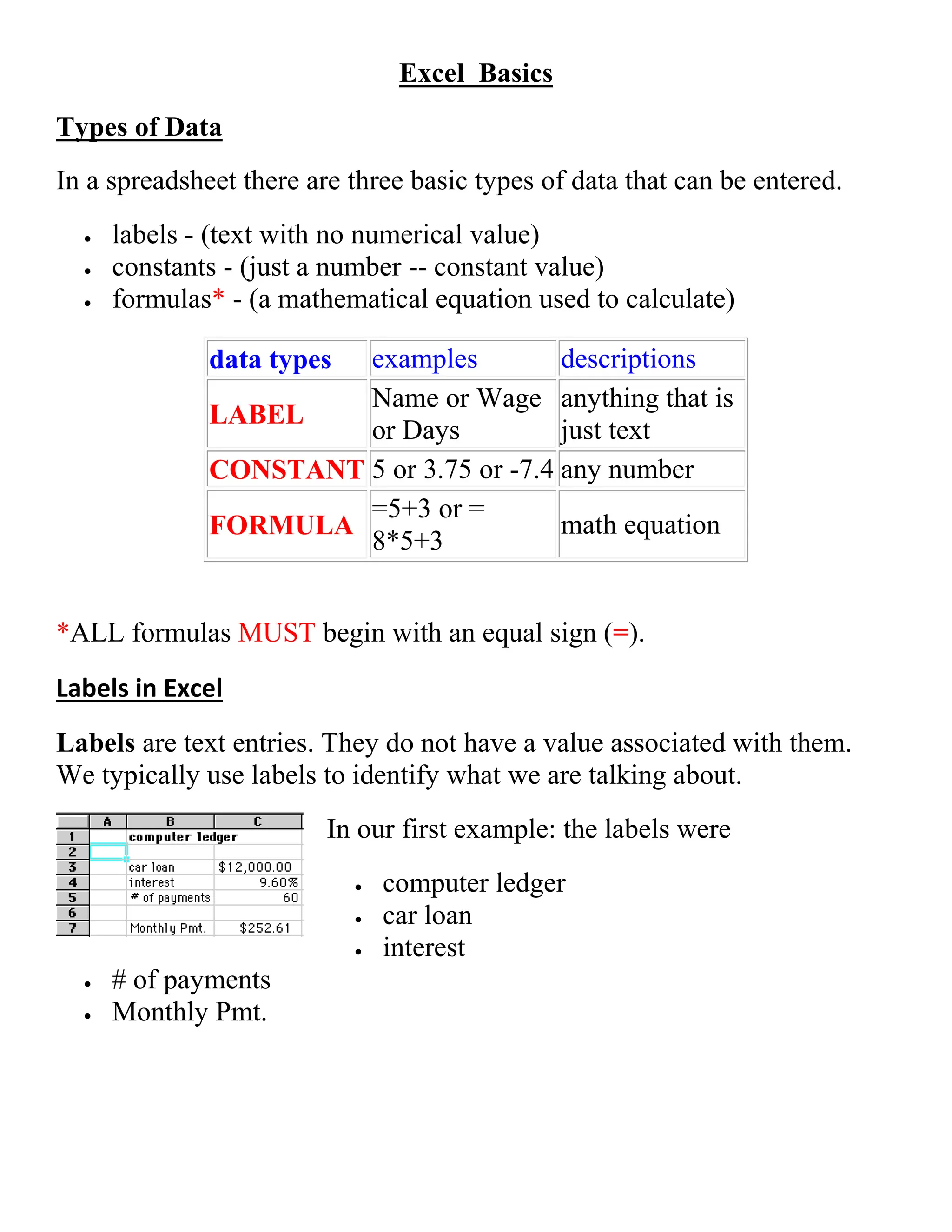
In our first example: the labels were
computer ledger
car loan
interest
# of payments
Monthly Pmt.
2.
Again, we uselabels to help identify what we are talking about. The labels
are NOT for the computer but rather for US so we can clarify what we are
doing.
Constants in Excel
Constants are entries that have a specific fixed value. If someone asks
you how old you are, you would answer with a specific answer. Sure,
other people will have different answers, but it is a fixed value for each
person.
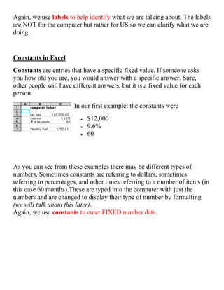
In our first example: the constants were
$12,000
9.6%
60
As you can see from these examples there may be different types of
numbers. Sometimes constants are referring to dollars, sometimes
referring to percentages, and other times referring to a number of items (in
this case 60 months).These are typed into the computer with just the
numbers and are changed to display their type of number by formatting
(we will talk about this later).
Again, we use constants to enter FIXED number data.
3.
Formulas in Excel
Formulasare entries that have an equation that calculates the value to
display. We DO NOT type in the numbers we are looking for; we type in
the equation. This equation will be updated upon the change or entry of
any data that is referenced in the equation.
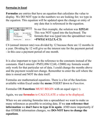
In our first example, the solution was $252.61
This was NOT typed into the keyboard. The
formula that was typed into the spreadsheet was:
=PMT(C4/12,C5,-C3)
C4 (annual interest rate) was divided by 12 because there are 12 months in
a year. Dividing by 12 will give us the interest rate for the payment period
- in this case a payment period of one month.
It is also important to type in the reference to the constants instead of the
constants. Had I entered =PMT(.096/12,60,-12000) my formula would
only work for that particular set of data. I could change the months above
and the payment would not change. Remember to enter the cell where the
data is stored and NOT the data itself.
Formulas are mathematical equations. There is a list of the functions
available within Excel under the menu INSERT down to Function.
Formulas OR Functions MUST BEGIN with an equal sign (=).
Again, we use formulas to CALCULATE a value to be displayed.
When we are entering formulas into a spreadsheet we want to make as
many references as possible to existing data. If we can reference that
information we don't have to type it in again. AND more importantly if
that OTHER information changes, we DO-NOT have to change the
equations.
4.
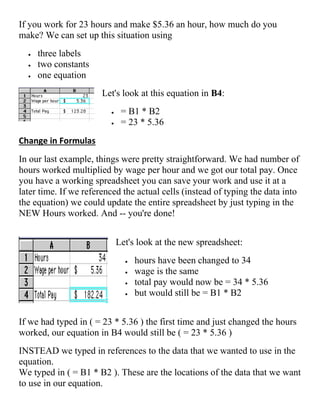
If you workfor 23 hours and make $5.36 an hour, how much do you
make? We can set up this situation using
three labels
two constants
one equation
Let's look at this equation in B4:
= B1 * B2
= 23 * 5.36
Change in Formulas
In our last example, things were pretty straightforward. We had number of
hours worked multiplied by wage per hour and we got our total pay. Once
you have a working spreadsheet you can save your work and use it at a
later time. If we referenced the actual cells (instead of typing the data into
the equation) we could update the entire spreadsheet by just typing in the
NEW Hours worked. And -- you're done!
Let's look at the new spreadsheet:
hours have been changed to 34
wage is the same
total pay would now be = 34 * 5.36
but would still be = B1 * B2
If we had typed in ( = 23 * 5.36 ) the first time and just changed the hours
worked, our equation in B4 would still be ( = 23 * 5.36 )
INSTEAD we typed in references to the data that we wanted to use in the
equation.
We typed in ( = B1 * B2 ). These are the locations of the data that we want
to use in our equation.
5.
Basic Math Functions
Spreadsheetshave many Math functions built into them. Of the most basic
operations are the standard multiply, divide, add and subtract. These
operations follow the order of operations (just like algebra). Let's look at
some examples.
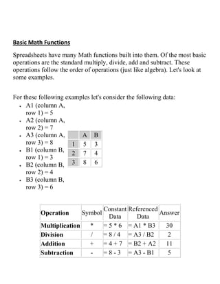
For these following examples let's consider the following data:
A1 (column A,
row 1) = 5
A2 (column A,
row 2) = 7
A3 (column A,
row 3) = 8
B1 (column B,
row 1) = 3
B2 (column B,
row 2) = 4
B3 (column B,
row 3) = 6
A B
1 5 3
2 7 4
3 8 6
Operation Symbol
Constant
Data
Referenced
Data
Answer
Multiplication * = 5 * 6 = A1 * B3 30
Division / = 8 / 4 = A3 / B2 2
Addition + = 4 + 7 = B2 + A2 11
Subtraction - = 8 - 3 = A3 - B1 5
6.
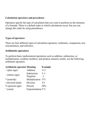
Calculation operators andprecedence
Operators specify the type of calculation that you want to perform on the elements
of a formula. There is a default order in which calculations occur, but you can
change this order by using parentheses.
Types of operators
There are four different types of calculation operators: arithmetic, comparison, text
concatenation, and reference.
Arithmetic operators
To perform basic mathematical operations such as addition, subtraction, or
multiplication; combine numbers; and produce numeric results, use the following
arithmetic operators.
Arithmetic operator Meaning Example
+ (plus sign) Addition 3+3
– (minus sign)
Subtraction
Negation
3–1
–1
* (asterisk) Multiplication 3*3
/ (forward slash) Division 3/3
% (percent sign) Percent 20%
^ (caret) Exponentiation 3^2
7.
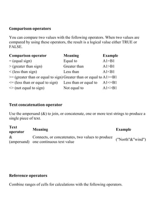
Comparison operators
You cancompare two values with the following operators. When two values are
compared by using these operators, the result is a logical value either TRUE or
FALSE.
Comparison operator Meaning Example
= (equal sign) Equal to A1=B1
> (greater than sign) Greater than A1>B1
< (less than sign) Less than A1<B1
>= (greater than or equal to sign) Greater than or equal to A1>=B1
<= (less than or equal to sign) Less than or equal to A1<=B1
<> (not equal to sign) Not equal to A1<>B1
Text concatenation operator
Use the ampersand (&) to join, or concatenate, one or more text strings to produce a
single piece of text.
Text
operator
Meaning Example
&
(ampersand)
Connects, or concatenates, two values to produce
one continuous text value
("North"&"wind")
Reference operators
Combine ranges of cells for calculations with the following operators.
8.
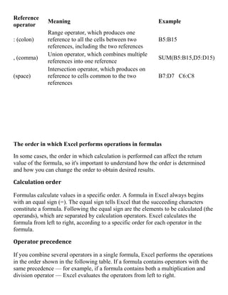
Reference
operator
Meaning Example
: (colon)
Rangeoperator, which produces one
reference to all the cells between two
references, including the two references
B5:B15
, (comma)
Union operator, which combines multiple
references into one reference
SUM(B5:B15,D5:D15)
(space)
Intersection operator, which produces on
reference to cells common to the two
references
B7:D7 C6:C8
The order in which Excel performs operations in formulas
In some cases, the order in which calculation is performed can affect the return
value of the formula, so it's important to understand how the order is determined
and how you can change the order to obtain desired results.
Calculation order
Formulas calculate values in a specific order. A formula in Excel always begins
with an equal sign (=). The equal sign tells Excel that the succeeding characters
constitute a formula. Following the equal sign are the elements to be calculated (the
operands), which are separated by calculation operators. Excel calculates the
formula from left to right, according to a specific order for each operator in the
formula.
Operator precedence
If you combine several operators in a single formula, Excel performs the operations
in the order shown in the following table. If a formula contains operators with the
same precedence — for example, if a formula contains both a multiplication and
division operator — Excel evaluates the operators from left to right.
9.
Operator Description
: (colon)
(singlespace)
, (comma)
Reference operators
– Negation (as in –1)
% Percent
^ Exponentiation
* and / Multiplication and division
+ and – Addition and subtraction
& Connects two strings of text (concatenation)
=
< >
<=
>=
<>
Comparison
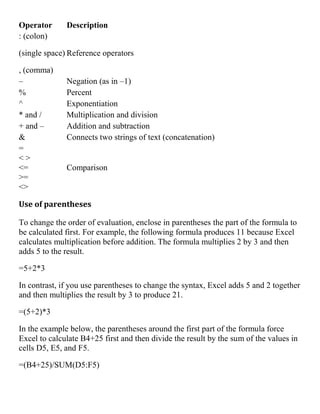
Use of parentheses
To change the order of evaluation, enclose in parentheses the part of the formula to
be calculated first. For example, the following formula produces 11 because Excel
calculates multiplication before addition. The formula multiplies 2 by 3 and then
adds 5 to the result.
=5+2*3
In contrast, if you use parentheses to change the syntax, Excel adds 5 and 2 together
and then multiplies the result by 3 to produce 21.
=(5+2)*3
In the example below, the parentheses around the first part of the formula force
Excel to calculate B4+25 first and then divide the result by the sum of the values in
cells D5, E5, and F5.
=(B4+25)/SUM(D5:F5)
10.
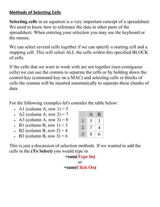
Methods of SelectingCells
Selecting cells in an equation is a very important concept of a spreadsheet.
We need to know how to reference the data in other parts of the
spreadsheet. When entering your selection you may use the keyboard or
the mouse.
We can select several cells together if we can specify a starting cell and a
stopping cell. This will select ALL the cells within this specified BLOCK
of cells.
If the cells that we want to work with are not together (non-contiguous
cells) we can use the comma to separate the cells or by holding down the
control-key (command key on a MAC) and selecting cells or blocks of
cells the comma will be inserted automatically to separate these chunks of
data.
For the following examples let's consider the table below:
A1 (column A, row 1) = 5
A2 (column A, row 2) = 7
A3 (column A, row 3) = 8
B1 (column B, row 1) = 3
B2 (column B, row 2) = 4
B3 (column B, row 3) = 6
A B
1 5 3
2 7 4
3 8 6
This is just a discussion of selection methods. If we wanted to add the
cells in the (To Select) you would type in
=sum(Type In)
or
=sum(Click On)
11.
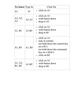
To Select TypeIn Click On
A1 A1 click on A1
A1, A2,
A3
A1:A3
click on A1
with button down
drag to A3
A1, B1 A1:B1
click on A1
with button down
drag to B1
A1, B3 A1, B3
click on A1
type in comma
(or hold down the control key
on a PC)
(or hold down the command
key on a MAC)
click on B3
A1, A2,
B1, B2
A1:B2
click on A1
with button down
drag to B2
12.
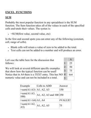
EXCEL FUNCTIONS
SUM
Probably themost popular function in any spreadsheet is the SUM
function. The Sum function takes all of the values in each of the specified
cells and totals their values. The syntax is:
=SUM(first value, second value, etc)
In the first and second spots you can enter any of the following (constant,
cell, range of cells).
Blank cells will return a value of zero to be added to the total.
Text cells can not be added to a number and will produce an error.
Let's use the table here for the discussion that
follows:
We will look at several different specific examples
that show how the typical function can be used!
Notice that in A4 there is a TEXT entry. This has NO
numeric value and can not be included in a total.
A
1 25
2 50
3 75
4 test
5
Example Cells to ADD Answer
=sum(A1:A3) A1, A2, A3 150
=sum(A1:A3,
100)
A1, A2, A3 and 100 250
=sum(A1+A4) A1, A4 #VALUE!
=sum(A1:A2,
A5)
A1, A2, A5 75
13.
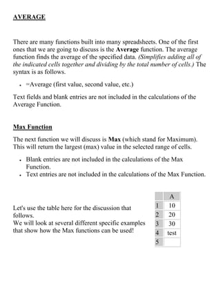
AVERAGE
There are manyfunctions built into many spreadsheets. One of the first
ones that we are going to discuss is the Average function. The average
function finds the average of the specified data. (Simplifies adding all of
the indicated cells together and dividing by the total number of cells.) The
syntax is as follows.
=Average (first value, second value, etc.)
Text fields and blank entries are not included in the calculations of the
Average Function.
Max Function
The next function we will discuss is Max (which stand for Maximum).
This will return the largest (max) value in the selected range of cells.
Blank entries are not included in the calculations of the Max
Function.
Text entries are not included in the calculations of the Max Function.
Let's use the table here for the discussion that
follows.
We will look at several different specific examples
that show how the Max functions can be used!
A
1 10
2 20
3 30
4 test
5
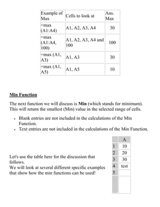
14.
Example of
Max
Cells tolook at
Ans.
Max
=max
(A1:A4)
A1, A2, A3, A4 30
=max
(A1:A4,
100)
A1, A2, A3, A4 and
100
100
=max (A1,
A3)
A1, A3 30
=max (A1,
A5)
A1, A5 10
Min Function
The next function we will discuss is Min (which stands for minimum).
This will return the smallest (Min) value in the selected range of cells.
Blank entries are not included in the calculations of the Min
Function.
Text entries are not included in the calculations of the Min Function.
Let's use the table here for the discussion that
follows.
We will look at several different specific examples
that show how the min functions can be used!
A
1 10
2 20
3 30
4 test
5
15.
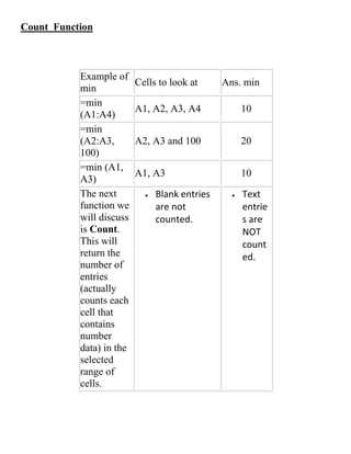
Count Function
Example of
min
Cellsto look at Ans. min
=min
(A1:A4)
A1, A2, A3, A4 10
=min
(A2:A3,
100)
A2, A3 and 100 20
=min (A1,
A3)
A1, A3 10
The next
function we
will discuss
is Count.
This will
return the
number of
entries
(actually
counts each
cell that
contains
number
data) in the
selected
range of
cells.
Blank entries
are not
counted.
Text
entrie
s are
NOT
count
ed.
16.
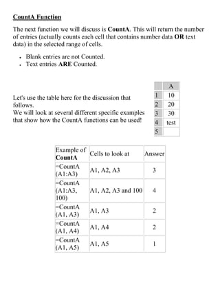
CountA Function
The nextfunction we will discuss is CountA. This will return the number
of entries (actually counts each cell that contains number data OR text
data) in the selected range of cells.
Blank entries are not Counted.
Text entries ARE Counted.
Let's use the table here for the discussion that
follows.
We will look at several different specific examples
that show how the CountA functions can be used!
A
1 10
2 20
3 30
4 test
5
Example of
CountA
Cells to look at Answer
=CountA
(A1:A3)
A1, A2, A3 3
=CountA
(A1:A3,
100)
A1, A2, A3 and 100 4
=CountA
(A1, A3)
A1, A3 2
=CountA
(A1, A4)
A1, A4 2
=CountA
(A1, A5)
A1, A5 1
17.
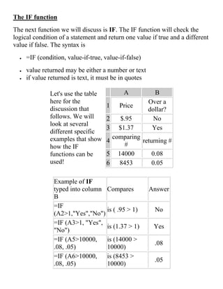
The IF function
Thenext function we will discuss is IF. The IF function will check the
logical condition of a statement and return one value if true and a different
value if false. The syntax is
=IF (condition, value-if-true, value-if-false)
value returned may be either a number or text
if value returned is text, it must be in quotes
Let's use the table
here for the
discussion that
follows. We will
look at several
different specific
examples that show
how the IF
functions can be
used!
A B
1 Price
Over a
dollar?
2 $.95 No
3 $1.37 Yes
4
comparing
#
returning #
5 14000 0.08
6 8453 0.05
Example of IF
typed into column
B
Compares Answer
=IF
(A2>1,"Yes","No")
is ( .95 > 1) No
=IF (A3>1, "Yes",
"No")
is (1.37 > 1) Yes
=IF (A5>10000,
.08, .05)
is (14000 >
10000)
.08
=IF (A6>10000,
.08, .05)
is (8453 >
10000)
.05
18.
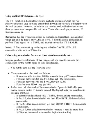
Using multiple IFstatements in Excel
The IF( ) function in Excel allows you to evaluate a situation which has two
possible outcomes (e.g. sales are greater than $1000) and calculate a different value
for each outcome. However, sometimes you need to work with situations where
there are more than two possible outcomes. That's where multiple, or nested, IF
functions come in.
Remember that the IF function works by evaluating a logical test - a calculation
which can only be TRUE or FALSE, or 1 or 0. It then includes a calculation to
perform if the logical test is TRUE, and another calculation if it is FALSE.
Nested IF functions work by replacing one or both of the TRUE/FALSE
calculations with another IF function.
Calculating commission for a sales team based on monthly sales
Imagine you have a sales team of five people, and you need to calculate their
commission for the month based on their sales figures.
You put the data into the following table:
Your commission plan works as follows:
o If someone sells less than $400 in a month, they get 7% commission.
o For sales between $400 and $750, they get 10% commission.
o For sales between $750 and $1000, they get 12.5%
o For sales over $1000, they get 16%
Rather than calculate each of these commission figures individually, you
decide to use a nested IF formula instead. The logical tests you would use in
this case are these:
o Is commission less than $400? If TRUE, then calculate commission.
o If FALSE, then is commission less than $750? If TRUE then calculate
commission.
o If FALSE, then is commission less than $1000? If TRUE then calculate
commission.
o If FALSE, then calculate commission (because it must be more than
$1000 - we don't need to do another logical test for this).
19.
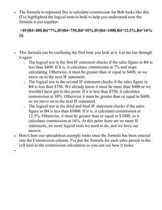
The formulato represent this to calculate commission for Bob looks like this
(I've highlighted the logical tests in bold to help you understand now the
formula is put together:
=IF(B4<400,B4*7%,IF(B4<750,B4*10%,IF(B4<1000,B4*12.5%,B4*16%
)))
This formula can be confusing the first time you look at it. Let me run through
it again.
o The logical test in the first IF statement checks if the sales figure in B4 is
less than $400. If it is, it calculates commission at 7% and stops
calculating. Otherwise, it must be greater than or equal to $400, so we
move on to the next IF statement.
o The logical test in the second IF statement checks if the sales figure in
B4 is less than $750. We already know it must be more than $400 or we
wouldn't have got to this point. If it is less than $750, it calculates
commission at 10%. Otherwise it must be greater than or equal to $400,
so we move on to the next IF statement.
o The logical test in the third and final IF statement checks if the sales
figure in B4 is less than $1000. If it is, it calculates commission at
12.5%. Otherwise, it must be greater than or equal to $1000, so it
calculates commission at 16%. At this point there are no more IF
statements, no more logical tests we need to do, and we have our
answer.
Here's how our spreadsheet example looks once the formula has been entered
into the Commission column. I've put the formula for each sales person in the
cell next to the commission calculation so you can see how it looks:
20.
Function Wizard.
In Excelthere is a help tool for functions called the Function Wizard.
There are two ways to get the function wizard. If you look at the
Standard Toolbar, the function wizard icon looks like the icon on the
right.
The other way to get to the function wizard is to go to the Menu INSERT
-- down to FUNCTION.
Either way you get there, at this point Excel will list all of the functions
available. Upon choosing the function, Excel will prompt you for the
information it needs to complete the function. Mini descriptions are
available for each of the cells. It is often necessary for you to understand
the functions in order to be able to figure out these descriptions.
Yeah, I know it would have been nice to know this earlier, but it is
important for you to understand how the functions work before you start
using the Function Wizard. It is faster to type the basic function in from
the keyboard as opposed to going through the steps of this tool.
COPYING FORMULAS
Sometimes when we enter a formula, we need to repeat the same formula
for many different cells. In the spreadsheet we can use the copy and paste
command. The cell locations in the formula are pasted relative to the
position we Copy them from.
21.
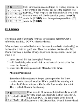
A B C
15 3 =A1+B1
2 8 2 =A2+B2
3 4 6 =A3+B3
4 3 8 =? + ?
Cells information is copied from its relative position. In
other words in the original cell (C1) the equation was
(A1+B1). When we paste the function it will look to the
two cells to the left. So the equation pasted into (C2)
would be (A2+B2). And the equation pasted into (C3)
would be (A3+B3).
FILL DOWN
If you have a lot of duplicate formulas you can also perform what is
referred to as a FILL DOWN. (discussed next).
Often we have several cells that need the same formula (in relationship) to
the location it is to be typed into. There is a short cut that is called Fill
Down. There are a number of ways to perform this operation. One of the
ways is to
1. select the cell that has the original formula
2. hold the shift key down and click on the last cell (in the series that
needs the formula)
3. under the edit menu go down to fill and over to down
Absolute Positioning
Sometimes it is necessary to keep a certain position that is not
relative to the new cell location. This is possible by inserting a $
before the Column letter or a $ before the Row number (or both).
This is called Absolute Positioning.
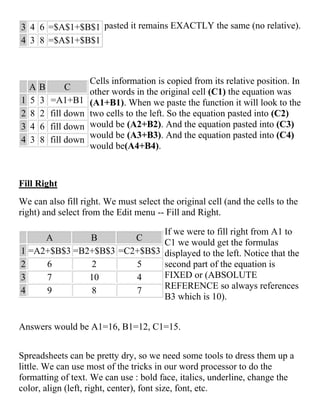
A B C
1 5 3 =$A$1+$B$1
2 8 2 =$A$1+$B$1
If we were to fill down with this formula we would
have the exact same formula in all of the cells C1,
C2, C3, and C4. The dollar signs Lock the cell
location to a FIXED position. When it is copied and
22.
3 4 6=$A$1+$B$1
4 3 8 =$A$1+$B$1
pasted it remains EXACTLY the same (no relative).
A B C
1 5 3 =A1+B1
2 8 2 fill down
3 4 6 fill down
4 3 8 fill down
Cells information is copied from its relative position. In
other words in the original cell (C1) the equation was
(A1+B1). When we paste the function it will look to the
two cells to the left. So the equation pasted into (C2)
would be (A2+B2). And the equation pasted into (C3)
would be (A3+B3). And the equation pasted into (C4)
would be(A4+B4).
Fill Right
We can also fill right. We must select the original cell (and the cells to the
right) and select from the Edit menu -- Fill and Right.
A B C
1 =A2+$B$3 =B2+$B$3 =C2+$B$3
2 6 2 5
3 7 10 4
4 9 8 7
If we were to fill right from A1 to
C1 we would get the formulas
displayed to the left. Notice that the
second part of the equation is
FIXED or (ABSOLUTE
REFERENCE so always references
B3 which is 10).
Answers would be A1=16, B1=12, C1=15.
Spreadsheets can be pretty dry, so we need some tools to dress them up a
little. We can use most of the tricks in our word processor to do the
formatting of text. We can use : bold face, italics, underline, change the
color, align (left, right, center), font size, font, etc.
23.
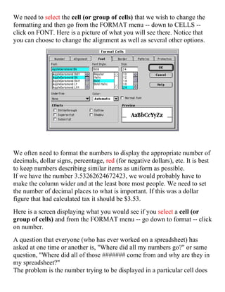
We need toselect the cell (or group of cells) that we wish to change the
formatting and then go from the FORMAT menu -- down to CELLS --
click on FONT. Here is a picture of what you will see there. Notice that
you can choose to change the alignment as well as several other options.
We often need to format the numbers to display the appropriate number of
decimals, dollar signs, percentage, red (for negative dollars), etc. It is best
to keep numbers describing similar items as uniform as possible.
If we have the number 3.53262624672423, we would probably have to
make the column wider and at the least bore most people. We need to set
the number of decimal places to what is important. If this was a dollar
figure that had calculated tax it should be $3.53.
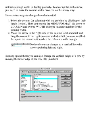
Here is a screen displaying what you would see if you select a cell (or
group of cells) and from the FORMAT menu -- go down to format -- click
on number.
A question that everyone (who has ever worked on a spreadsheet) has
asked at one time or another is, "Where did all my numbers go?" or same
question, "Where did all of those ####### come from and why are they in
my spreadsheet?"
The problem is the number trying to be displayed in a particular cell does
24.
not have enoughwidth to display properly. To clear up the problem we
just need to make the column wider. You can do this many ways.
Here are two ways to change the column width
1. Select the column (or columns) with the problem by clicking on their
labels (letters). Then you choose the MENU FORMAT. Go down to
COLUMN and over to WIDTH and type in a new number for the
column width.
2. Move the arrow to the right side of the column label and click and
drag the mouse to the right (to make wider) or left (to make smaller).
Let up on the mouse button when the column is wide enough.
Notice the cursor changes to a vertical line with
arrows pointing left and right.
In many spreadsheets you can also change the vertical height of a row by
moving the lower edge of the row title (number).
25.
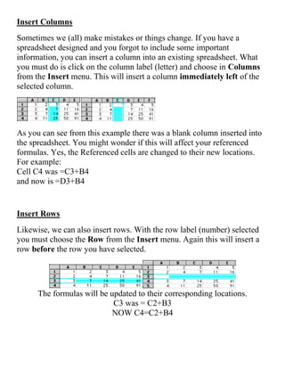
Insert Columns
Sometimes we(all) make mistakes or things change. If you have a
spreadsheet designed and you forgot to include some important
information, you can insert a column into an existing spreadsheet. What
you must do is click on the column label (letter) and choose in Columns
from the Insert menu. This will insert a column immediately left of the
selected column.
As you can see from this example there was a blank column inserted into
the spreadsheet. You might wonder if this will affect your referenced
formulas. Yes, the Referenced cells are changed to their new locations.
For example:
Cell C4 was =C3+B4
and now is =D3+B4
Insert Rows
Likewise, we can also insert rows. With the row label (number) selected
you must choose the Row from the Insert menu. Again this will insert a
row before the row you have selected.
The formulas will be updated to their corresponding locations.
C3 was = C2+B3
NOW C4=C2+B4
26.
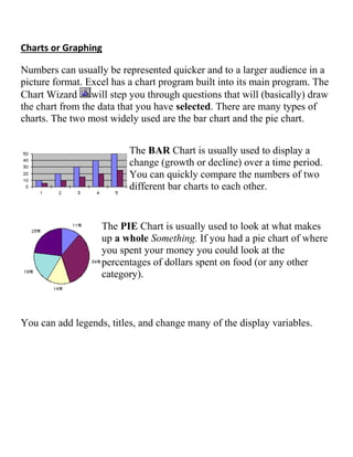
Charts or Graphing
Numberscan usually be represented quicker and to a larger audience in a
picture format. Excel has a chart program built into its main program. The
Chart Wizard will step you through questions that will (basically) draw
the chart from the data that you have selected. There are many types of
charts. The two most widely used are the bar chart and the pie chart.
The BAR Chart is usually used to display a
change (growth or decline) over a time period.
You can quickly compare the numbers of two
different bar charts to each other.
The PIE Chart is usually used to look at what makes
up a whole Something. If you had a pie chart of where
you spent your money you could look at the
percentages of dollars spent on food (or any other
category).
You can add legends, titles, and change many of the display variables.


![Spreadsheets[1]](https://cdn.slidesharecdn.com/ss_thumbnails/spreadsheets1-150131022908-conversion-gate01-thumbnail.jpg?width=640&height=640&fit=bounds)