2 dimentional steady state conduction.pdf

Chapter 2: Two-Dimensional, Steady-State Conduction
Section 2.1: Shape Factors
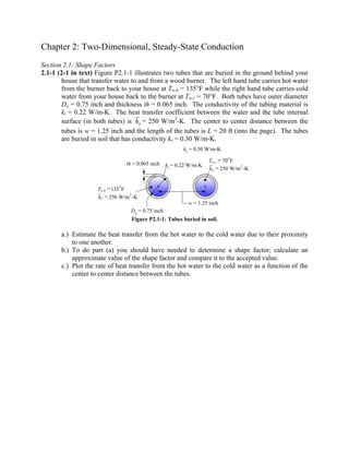
2.1-1 (2-1 in text) Figure P2.1-1 illustrates two tubes that are buried in the ground behind your
house that transfer water to and from a wood burner. The left hand tube carries hot water
from the burner back to your house at Tw,h = 135°F while the right hand tube carries cold
water from your house back to the burner at Tw,c = 70°F. Both tubes have outer diameter
Do = 0.75 inch and thickness th = 0.065 inch. The conductivity of the tubing material is
kt = 0.22 W/m-K. The heat transfer coefficient between the water and the tube internal
surface (in both tubes) is w
h = 250 W/m2
-K. The center to center distance between the
tubes is w = 1.25 inch and the length of the tubes is L = 20 ft (into the page). The tubes
are buried in soil that has conductivity ks = 0.30 W/m-K.
kt = 0.22 W/m-K
th = 0.065 inch
Do = 0.75 inch
w = 1.25 inch
ks = 0.30 W/m-K
,
2
135 F
250 W/m -K
w h
w
T
h
= °
=
,
2
70 F
250 W/m -K
w c
w
T
h
= °
=
Figure P2.1-1: Tubes buried in soil.
a.) Estimate the heat transfer from the hot water to the cold water due to their proximity
to one another.
b.) To do part (a) you should have needed to determine a shape factor; calculate an
approximate value of the shape factor and compare it to the accepted value.
c.) Plot the rate of heat transfer from the hot water to the cold water as a function of the
center to center distance between the tubes.

2.1-2 Currently, the low-pressure steam exhausted from a steam turbine at the power plant is
condensed by heat transfer to cooling water. An alternative that has been proposed is to
transport the steam via an underground pipe to a large building complex and use the
steam for space heating. You have been asked to evaluate the feasibility of this proposal.
The building complex is located 0.2 miles from the power plant. The pipe is made of
uninsulated PVC (thermal conductivity of 0.19 W/m-K) with an inner diameter of 8.33 in
and wall thickness 0.148 in. The pipe will be buried underground at a depth of 4 ft in soil
that has an estimated thermal conductivity of 0.5 W/m-K. The steam leaves the power
plant at 6.5 lbm/min, 8 psia with a 95% quality. The outdoor temperature is 5°F.
Condensate is returned to the power plant in a separate pipe as, approximately, saturated
liquid at 8 psia.
a.) Neglecting the inevitable pressure loss, estimate the state of the steam that is provided
to the building complex.
b.) Are the thermal losses experienced in the underground pipe transport process
significant in your opinion? Do you recommend insulating this pipe?
c.) Provide a sanity check on the shape factor that you used to solve this problem.

2.1-3 (2-2 in text) A solar electric generation system (SEGS) employs molten salt as both the
energy transport and storage fluid. The molten salt is heated to 500°C and stored in a
buried semi-spherical tank. The top (flat) surface of the tank is at ground level. The
diameter of the tank before insulation is applied 14 m. The outside surfaces of the tank
are insulated with 0.30 m thick fiberglass having a thermal conductivity of 0.035 W/m-K.
Sand having a thermal conductivity of 0.27 W/m-K surrounds the tank, except on its top
surface. Estimate the rate of heat loss from this storage unit to the 25°C surroundings.

2.1-4 A square extrusion is L = 1 m long and has outer dimension W = 3 cm. There is a D = 1
cm diameter hole aligned with the center of the extrusion. The material has conductivity
k = 0.5 W/m-K. The external surface of the extrusion is exposed to air at Ta = 20ºC with
heat transfer coefficient a
h = 50 W/m2
-K. The inner surface of the extrusion is exposed
to water at Tw = 80 ºC with heat transfer coefficient w
h = 150 W/m2
-K.
a.) Determine the rate of heat transfer between the water and the air.
b.) Carry out a sanity check on the value of the shape factor that you used in (a).

2.1-5 A pipe carrying water for a ground source heat pump is buried horizontally in soil with
conductivity k = 0.4 W/m-K. The center of the pipe is W = 6 ft below the surface of the
ground. The pipe has inner diameter Di = 1.5 inch and outer diameter Do = 2 inch. The
pipe is made of material with conductivity kp = 1.5 W/m-K. The water flowing through
the pipe has temperature Tw = 35ºF with heat transfer coefficient w
h = 200 W/m-K. The
temperature of the surface of the soil is Ts = 0ºF.
a.) Determine the rate of heat transfer between the water and the air per unit length of
pipe.
b.) Plot the heat transfer as a function of the depth of the pipe.
c.) Carry out a sanity check on the value of the shape factor that you used in (a).

Section 2.2: Separation of Variables Solutions
2.2-1 You are evaluating a technique for controlling the properties of welded joints by using
aggressive liquid cooling. Figure P2.2-1 illustrates a cut-away view of two plates that are
being welded together. Both edges of the plate are clamped and effectively held at
temperatures Ts = 25°C. The top of the plate is exposed to a heat flux that varies with
position x, measured from joint, according to: ( ) ( )
exp /
m j j
q x q x L
′′ ′′
= −
where j
q′′
=1x106
W/m2
is the maximum heat flux (at the joint, x = 0) and Lj = 2.0 cm is a measure of the
extent of the heat flux. The back side of the plates are exposed to aggressive liquid
cooling by a jet of fluid at Tf = -35°C with h = 5000 W/m2
-K. A half-symmetry model
of the problem is shown in Figure P2.2-1. The thickness of the plate is b = 3.5 cm and
the width of a single plate is W = 8.5 cm. You may assume that the welding process is
steady-state and 2-D. You may neglect convection from the top of the plate. The
conductivity of the plate material is k = 38 W/m-K.
heat flux
joint
impingement cooling with liquid jets
both edges are
clamped and held
at fixed temperature
m
q′′

25 C
s
T = °
x
y
W = 8.5 cm
b = 3.5 cm
2
35 C
500 W/m -K
f
T
h
= − °
=
k = 38 W/m-K
Figure P2-2-1: Welding process and half-symmetry model of the welding process.
a.) Develop a separation of variables solution to the problem. Implement the solution in
EES and prepare a plot of the temperature as a function of x at y = 0, 1.0, 2.0, 3.0, and
3.5 cm.
b.) Prepare a contour plot of the temperature distribution.

2.2-2 Figure P2.2-2 illustrates a thin plate that is exposed to air on upper and lower surfaces.
The heat transfer coefficient between the top and bottom surfaces is h and the air
temperature is Tf. The thickness of the plate is th and its width and height are a and b,
respectively. The conductivity of the plate is k. The top edge is fixed at a uniform
temperature, T1. The right edge is fixed at a different, uniform temperature, T2. The left
edge of the plate is insulated. The bottom edge of the plate is exposed to a heat flux, q′′
.
This problem should be done on paper.
T1
b
a
k
x
y
T2
q′′

th
, f
h T
, f
h T
Figure P.2.2-2: Thin plate exposed to air.
a.) The temperature distribution within the plate can be considered 2-D (i.e., temperature
variations in the z-direction can be neglected) if the plate is thin and conductive.
How would you determine if this approximation is valid?
b.) Derive the partial differential equation and boundary conditions that would need to be
solved in order to obtain an analytical solution to this problem.

2.2-3 (2-3 in text) You are the engineer responsible for a simple device that is used to measure
heat transfer coefficient as a function of position within a tank of liquid (Figure P2.2-3).
The heat transfer coefficient can be correlated against vapor quality, fluid composition,
and other useful quantities. The measurement device is composed of many thin plates of
low conductivity material that are interspersed with large, copper interconnects. Heater
bars run along both edges of the thin plates. The heater bars are insulated and can only
transfer energy to the plate; the heater bars are conductive and can therefore be assumed
to come to a uniform temperature as a current is applied. This uniform temperature is
assumed to be applied to the top and bottom edges of the plates. The copper
interconnects are thermally well-connected to the fluid; therefore, the temperature of the
left and right edges of each plate are equal to the fluid temperature. This is convenient
because it isolates the effect of adjacent plates from one another which allows each plate
to measure the local heat transfer coefficient. Both surfaces of the plate are exposed to
the fluid temperature via a heat transfer coefficient. It is possible to infer the heat transfer
coefficient by measuring heat transfer required to elevate the heater bar temperature a
specified temperature above the fluid temperature.
2
top and bottom surfaces exposed to fluid
20 C, 50 W/m -K
T h
∞ = ° =
plate:
k = 20 W/m-K
th = 0.5 mm
a = 20 mm
b = 15 mm
heater bar, 40 C
h
T = °
copper interconnet, 20 C
T∞ = °
Figure P2.2-3: Device to measure heat transfer coefficient as a function of position.
The nominal design of an individual heater plate utilizes metal with k = 20 W/m-K, th =
0.5 mm, a = 20 mm, and b = 15 mm (note that a and b are defined as the half-width and
half-height of the heater plate, respectively, and th is the thickness as shown in Figure P2-
3). The heater bar temperature is maintained at Th = 40ºC and the fluid temperature is T∞
= 20ºC. The nominal value of the average heat transfer coefficient is h = 50 W/m2
-K.
a.) Develop an analytical model that can predict the temperature distribution in the plate
under these nominal conditions.
b.) The measured quantity is the rate of heat transfer to the plate from the heater ( h
q
) and
therefore the relationship between h
q
and h (the quantity that is inferred from the
heater power) determines how useful the instrument is. Determine the heater power.
c.) If the uncertainty in the measurement of the heater power is h
q
δ = 0.01 W, estimate
the uncertainty in the measured heat transfer coefficient ( h
δ ).

2.2-4 Figure P2.2-4(a) illustrates a proposed device to measure the local heat transfer
coefficient from a surface undergoing a boiling heat transfer process. Micro-scale heaters
and temperature sensors are embedded in a substrate in a regularly spaced array, as
shown.
heaters
temperature
sensors
computational
domain
evaporating fluid
Figure P2.2-4(a): An array of micro-scale heaters and temperature sensors embedded in a substrate.
The heaters are activated, producing a heat flux that is removed primarily from the
surface of the substrate exposed to evaporating fluid. The temperature sensors are
embedded in sets of two located very near the surface. Each set of thermocouples are
used to infer the local heat flux to the surface ( s
q′′
) and the surface temperature (Ts); these
quantities are sufficient to measure the heat transfer coefficient. A half-symmetry model
of the region of the substrate between two adjacent heaters (see Figure 2.2-4(a)) is shown
in Figure P2.2-4(b).
x
y
y1 = 1.9 mm
y2 = 1.8 mm
W = 5 mm
b = 2 mm
2
20 C
2500 W/m -K
T
h
∞
= °
=
k = 3.5 W/m-K
5 2
1x10 W/m
h
q′′ =

Figure P2.2-4(b): A half-symmetry model of the region of the substrate between two adjacent
heaters.
The thickness of the substrate is b = 2 mm and the half-width between adjacent heaters is
W = 5 mm. The substrate has conductivity k = 3.5 W/m-K and you may assume that the
presence of the temperature sensors does not affect the temperature distribution. The heat
flux exposed to the computational domain at x = W is h
q′′
= 1x105
W/m2
. The heat
transfer coefficient between the evaporating fluid at T∞ = 20ºC and the surface is h =
2500 W/m2
-K.
a.) Develop a separation of variables solution based on the computational domain shown
in Figure P2.2-4(b). Implement your solution in EES.
b.) Prepare a contour plot of the temperature distribution in the substrate.

The position of temperature sensors #1 and #2 at a particular value of x are y1 = 1.9 mm
and y2 = 1.8 mm, respectively (see Figure P2.2-4(b)). The surface temperature
measurement extracted from these measured temperatures is associated with a linear
extrapolation to the surface at y = 0:
( )
( )
( )
2
, 2 1 2
1 2
s m
b y
T T T T
y y
−
= + −
−
(1)
The heat flux measurement extracted from these measured temperatures is obtained from
Fourier's law according to:
( )
( )
2 1
,
1 2
s m
T T
q k
y y
−
′′ =
−
(2)
c.) What is the heat transfer coefficient measured by the device at x/W = 0.5? That is,
based on the temperatures T1 and T2 predicted by your model at x/W = 0.5, calculate
the measured heat transfer coefficient according to:
( )
,
,
s m
m
s m
q
h
T T∞
′′
=
−

(3)
and determine the discrepancy of your measurement relative to the actual heat
transfer coefficient.
d.) Plot the % error associated with the device configuration (i.e., the discrepancy
between the measured and actual heat transfer coefficient from part (c)) as a function
of axial position, x.

2.2-5 Three heater blocks provide heat to the back-side of a fin array that must be tested, as
shown in Figure P2.2-5.
L = 7 cm
x
y
th = 1 cm
k = 30 W/m-K
d = 4 cm
c = 1 cm
4 2
1 3x10 W/m
q′′=

4 2
2 3x10 W/m
q′′ =

2
20 W/m -K
20 C
h
T∞
=
= °
2
2
,
2
,
35 W/m -K
35 C
150
8 cm
0.8 cm
0.85
f
f
fins
s fin
b fin
fin
h
T
N
A
A
η
=
= °
=
=
=
=
Figure P2.2-5: An array of fins installed on a base plate energized by three heater blocks.
The fins are installed on a base plate that has half-width of L= 7 cm, thickness of th = 1
cm, and width W = 20 cm (into the page). The base plate material has conductivity k =
30 W/m-K. The edge of the base plate (at x = L) is exposed to air at T∞ = 20°C with heat
transfer coefficient h = 20 W/m2
-K. The middle of the plate (at x = 0) is a line of
symmetry and can be modeled as being adiabatic. The bottom of the plate (at y = 0) has
an array of Nfin = 150 fins installed. Each fin has surface area As,fin= 8 cm2
, base area Ab,fin
= 0.8 cm2
, and efficiency ηfin = 0.85. The fin and the base material are exposed to fluid at
Tf = 35°C with heat transfer coefficient f
h = 20 W/m2
-K. The top of the plate (at y = th)
is exposed to the heat flux from the heater blocks. The heat flux is distributed according
to:
( )
( )
1
2
if
0 if
if
y th
q x c
q c x d c
q x d c
=
⎧ ′′
⎪
′′ = +
⎨
⎪ ′′ +
⎩

where 1
q′′
= 3x104
W/m2
, 2
q′′
= 3x104
W/m2
, c = 1 cm and d = 4 cm.
a.) Determine an effective heat transfer coefficient that can be applied to the surface at y
= th in order to capture the combined effect of the fins and the unfinned base area.
b.) Develop a separation of variables solution for the temperature distribution within the
fin base material.
c.) Prepare a plot showing the temperature as a function of x at various values of y.
d.) The goal of the base plate is to provide an uniform heat flow to each fin. Assess the
performance of the base plate by plotting the rate of heat flux transferred to the fluid
as a function of x at y = 0.
e.) Overlay on your plot for (d) the rate of heat flux transferred to the fluid for various
values of the base plate conductivity.

2.2-6 (2-4 in text) A laminated composite structure is shown in Figure P2.2-6.
W = 6 cm
H = 3 cm
2
10000W/m
q′′ =

20 C
set
T = °
20 C
set
T = °
kx = 50 W/m-K
ky = 4 W/m-K
Figure P2.2-6: Composite structure exposed to a heat flux.
The structure is anisotropic. The effective conductivity of the composite in the x-
direction is kx = 50 W/m-K and in the y-direction it is ky = 4 W/m-K. The top of the
structure is exposed to a heat flux of q′′
= 10,000 W/m2
. The other edges are maintained
at Tset = 20°C. The height of the structure is H = 3 cm and the half-width is W = 6 cm.
a.) Develop a separation of variables solution for the 2-D steady-state temperature
distribution in the composite.

Section 2.3: Advanced Separation of Variables Solutions
2.3-1 (2-5 in text) Figure P2.3-1 illustrates a pipe that connects two tanks of liquid oxygen on a
spacecraft. The pipe is subjected to a heat flux, q′′
= 8,000 W/m2
, which can be assumed
to be uniformly applied to the outer surface of the pipe and entirely absorbed. Neglect
radiation from the surface of the pipe to space. The inner radius of the pipe is rin = 6 cm,
the outer radius of the pipe is rout = 10 cm, and the half-length of the pipe is L = 10 cm.
The ends of the pipe are attached to the liquid oxygen tanks and therefore are at a uniform
temperature of TLOx = 125 K. The pipe is made of a material with a conductivity of k =
10 W/m-K. The pipe is empty and therefore the internal surface can be assumed to be
adiabatic.
rin = 6 cm
rout = 10 cm
2
8,000 W/m
s
q′′ =

k = 10 W/m-K
L = 10 cm
TLOx = 125 K
Figure P2.3-1: Cryogen transfer pipe connecting two liquid oxygen tanks.
a.) Develop an analytical model that can predict the temperature distribution within the
pipe. Prepare a contour plot of the temperature distribution within the pipe.

2.3-2 (2-6 in text) Figure P2.3-2 illustrates a cylinder that is exposed to a concentrated heat flux
at one end.
rout = 200 μm
rexp = 21 μm
2
1500 W/cm
q′′ =

k = 168 W/m-K
extends to infinity
20 C
s
T = °
adiabatic
Figure P2.3-2: Cylinder exposed to a concentrated heat flux at one end.
The cylinder extends infinitely in the x-direction. The surface at x = 0 experiences a
uniform heat flux of q′′
= 1500 W/cm2
for r rexp = 21 μm and is adiabatic for rexp r
rout where rout = 200 μm is the outer radius of the cylinder. The outer surface of the
cylinder is maintained at a uniform temperature of Ts = 20ºC. The conductivity of the
cylinder material is k = 168 W/m-K.
a.) Develop a separation of variables solution for the temperature distribution within the
cylinder. Plot the temperature as a function of radius for various values of x.
b.) Determine the average temperature of the cylinder at the surface exposed to the heat
flux.
c.) Define a dimensionless thermal resistance between the surface exposed to the heat
flux and Ts. Plot the dimensionless thermal resistance as a function of rout/rin.
d.) Show that your plot from (c) does not change if the problem parameters (e.g., Ts, k,
etc.) are changed.

2.3-3 A disk-shaped window in an experiment is shown in Figure P2.3-3.
Rw = 3 cm
th = 1 cm
2
1000 W/m
rad
q′′ =

25 C
edge
T = °
2
50 W/m -K
20 C
h
T∞
=
= °
k = 1.2 W/m-K
x
r
Figure P2.3-3: Window.
The inside of the window (the surface at x = 0) is exposed to vacuum and therefore does
not experience any convection. However, this surface is exposed to a radiation heat flux
rad
q′′
= 1000 W/m2
. The window is assumed to be completely opaque to this radiation and
therefore it is absorbed at x = 0. The edge of the window at Rw = 3 cm is maintained at a
constant temperature Tedge = 25°C. The outside of the window (the surface at x = th) is
cooled by air at T∞ = 20°C with heat transfer coefficient h = 50 W/m2
-K. The
conductivity of the window material is k = 1.2 W/m-K.
a.) Is the extended surface approximation appropriate for this problem? That is, can the
temperature in the window be approximated as being 1-D in the radial direction?
Justify your answer.
b.) Assume that your answer to (a) is no. Develop a 2-D separation of variables solution
to this problem.
c.) Plot the temperature as a function of r for various values of x.
d.) Prepare a contour plot of the temperature in the window.

2.3-4 Reconsider Problem 2.3-3. The window is not opaque to the radiation but does absorb
some of it. The radiation that is absorbed is transformed to thermal energy. The
volumetric rate of thermal energy generation is given by: ( )
exp
rad
g q x
α α
′′′ ′′
= −
where α
= 100 m-1
is the absorption coefficient. The radiation that is not absorbed is transmitted.
Otherwise the problem remains the same.
a.) Develop a separation of variables solution to this problem using the techniques
discussed in Section 2.3.
b.) Plot the temperature as a function of r for various values of x.
c.) Show that your solution limits to the solution from Problem 2.3-3 in the limit that α
→ ∞.

Section 2.4: Superposition
2.4-1 (2-7 in text) The plate shown in Figure P2.4-1 is exposed to a uniform heat flux q′′
= 1x105
W/m2
along its top surface and is adiabatic at its bottom surface. The left side of the plate
is kept at TL = 300 K and the right side is at TR = 500 K. The height and width of the
plate are H = 1 cm and W = 5 cm, respectively. The conductivity of the plate is k = 10
W/m-K.
x
y
5 2
1x10 W/m
q′′ =

TL = 300 K
TR = 500 K
W = 5 cm
H = 1 cm
k = 10 W/m-K
Figure P2.4-1: Plate.
a.) Derive an analytical solution for the temperature distribution in the plate.
b.) Implement your solution in EES and prepare a contour plot of the temperature.

Section 2.5: Numerical Solutions to Steady-State 2-D Problems using EES
2.5-1 (2-8 in text) Figure P2.5-1 illustrates an electrical heating element that is affixed to the
wall of a chemical reactor. The element is rectangular in cross-section and very long
(into the page). The temperature distribution within the element is therefore two-
dimensional, T(x, y). The width of the element is a = 5.0 cm and the height is b = 10.0
cm. The three edges of the element that are exposed to the chemical (at x = 0, y = 0, and
x = a) are maintained at a temperature Tc = 200°C while the upper edge (at y = b) is
affixed to the well-insulated wall of the reactor and can therefore be considered adiabatic.
The element experiences a uniform volumetric rate of thermal energy generation, g′′′
=
1x106
W/m3
. The conductivity of the material is k = 0.8 W/m-K.
reactor wall
y
x
6 3
0.8 W/m-K
1x10 W/m
k
g
=
′′′ =

b = 10 cm
a = 5 cm
200 C
c
T = °
200 C
c
T = °
200 C
c
T = °
Figure P2.5-1: Electrical heating element.
a.) Develop a 2-D numerical model of the element using EES.
b.) Plot the temperature as a function of x at various values of y. What is the maximum
temperature within the element and where is it located?
c.) Prepare a reality check to show that your solution behaves according to your physical
intuition. That is, change some aspect of your program and show that the results
behave as you would expect (clearly describe the change that you made and show the
result).

2.5-2 Figure P2.5-2 illustrates a composite material that is being machined on a lathe.
H = 3 cm
W = 12 cm
20 C
chuck
T = °
depends on
20 C
h RS
T∞ = °
composite
thins = 100 μm
kins = 1.5 W/m-K
thm = 200 μm
km = 35 W/m-K
l
q′′

x
y
Figure P2.5-2: Composite material being machined on a lathe.
The composite is composed of alternating layers of insulating material and metal. The
insulating layers have thickness thins= 100 μm and conductivity kins = 1.5 W/m-K. The
metal layers have thickness thm = 200 μm and conductivity km = 35 W/m-K. The
workpiece is actually cylindrical and rotating. However, because the radius is large
relative to it thickness and there are no circumferential variations we can model the
workpiece as a 2-D problem in Cartesian coordinates, x and y, as shown in Figure 2.5-2.
The width of the workpiece is W = 12 cm and the thickness is H = 3 cm. The left surface
of the workpiece at x = 0 is attached to the chuck and therefore maintained at Tchuck =
20°C. The inner surface at y = 0 is insulated. The outer surface (at y = H) and right
surface (at x = W) are exposed to air at T∞ = 20°C with heat transfer coefficient h that
depends on the rotational speed of the chuck, RS in rev/min, according to:
2
2
2 2
W min
2
m K rev
h RS
⎡ ⎤
= ⎢ ⎥
⎣ ⎦
In order to extend the life of the tool used for the machining process, the workpiece is
preheated by applying laser power to the outer surface. The heat flux applied by the laser
depends on the rotational speed and position according to:
2
exp - c
l
x x
q a RS
pw
⎡ ⎤
⎛ ⎞
−
′′= ⎢ ⎥
⎜ ⎟
⎢ ⎥
⎝ ⎠
⎣ ⎦

where a = 5000 W-min/m2
-rev, xc = 8 cm, and pw = 1 cm.
a.) What is the effective thermal conductivity of the composite in the x- and y-directions?
b.) Develop a 2-D numerical model of the workpiece in EES. Plot the temperature as a
function of x at various values of y, including at least y = 0, H/2, and H.

c.) Plot the maximum temperature in the workpiece as a function of the rotational speed,
RS. If the objective is to preheat the material to its maximum possible temperature,
then what is the optimal rotational speed?

2.5-3 Figure P2.5-3 illustrates a heater that extends from a wall into fluid that is to be heated.
Figure P2.5-3: Heater.
Assume that the tip of the heater is insulated and that the width (W) is much larger than
the thickness (th) so that convection from the edges can be neglected. The length of the
heater is L = 5.0 cm. The base temperature is Tb = 20ºC and the heater experiences
convection with fluid at T∞= 100ºC with average heat transfer coefficient, h = 100 W/m2
-
K. The heater is th = 3.0 cm thick and has conductivity k = 1.5 W/m-K. The heater
experiences a uniform volumetric generation of g′′′
= 5x105
W/m3
.
a.) Develop a numerical solution for the temperature distribution in the heater using a
finite difference technique.
b.) Use the numerical solution to predict and plot the temperature distribution in the
heater.
c.) Use the numerical solution to predict the heater efficiency; the heater efficiency is
defined as the ratio of the rate of heat transfer to the fluid to the total rate of thermal
energy generation in the fin.
d.) Plot the heater efficiency as a function of the length for various values of the
thickness. Explain your plot.

Section 2.6: Finite-Difference Solutions to Steady-State 2-D Problems using MATLAB
2.6-1 (2-9 in text) Figure P2.6-1 illustrates a cut-away view of two plates that are being welded
together. Both edges of the plate are clamped and effectively held at temperatures Ts =
25°C. The top of the plate is exposed to a heat flux that varies with position x, measured
from joint, according to: ( ) ( )
exp /
m j j
q x q x L
′′ ′′
= −
where j
q′′
=1x106
W/m2
is the
maximum heat flux (at the joint, x = 0) and Lj = 2.0 cm is a measure of the extent of the
heat flux. The back side of the plates are exposed to liquid cooling by a jet of fluid at Tf
= -35°C with h = 5000 W/m2
-K. A half-symmetry model of the problem is shown in
Figure P2.6-1. The thickness of the plate is b = 3.5 cm and the width of a single plate is
W = 8.5 cm. You may assume that the welding process is steady-state and 2-D. You may
neglect convection from the top of the plate. The conductivity of the plate material is k =
38 W/m-K.
heat flux
joint
both edges are held at fixed temperature
impingement cooling
y
x
m
q′′
k = 38 W/m-K
W = 8.5 cm
b = 3.5 cm
25 C
s
T = °
2
5000 W/m -K, 35 C
f
h T
= = − °
Figure P2.6-1: Welding process and half-symmetry model of the welding process.
a.) Develop a separation of variables solution to the problem (note, this was done
previously in Problem 2.2-1). Implement the solution in EES and prepare a plot of
the temperature as a function of x at y = 0, 1.0, 2.0, 3.0, and 3.5 cm.
c.) Develop a numerical model of the problem. Implement the solution in MATLAB and
prepare a contour or surface plot of the temperature in the plate.
d.) Plot the temperature as a function of x at y = 0, b/2, and b and overlay on this plot the
separation of variables solution obtained in part (a) evaluated at the same locations.

2.6-2 Prepare a solution to Problem 2.3-3 using a finite difference technique.
a.) Plot the temperature as a function of r for various values of x.
b.) Prepare a contour plot of the temperature in the window.
c.) Verify that your solution agrees with the analytical solution from Problem 2.3-3.

2.6-3 Prepare a solution to Problem 2.3-4 using a finite difference technique.
a.) Plot the temperature as a function of r for various values of x.
b.) Prepare a contour plot of the temperature in the window.
c.) Verify that your solution agrees with the analytical solution from Problem 2.3-4.

Section 2.7: Finite-Element Solutions to Steady-State 2-D Problems using FEHT
2.7-1 (2-10 in text) Figure P2.7-1(a) illustrates a double paned window. The window consists of
two panes of glass each of which is tg = 0.95 cm thick and W = 4 ft wide by H = 5 ft high.
The glass panes are separated by an air gap of g = 1.9 cm. You may assume that the air is
stagnant with ka = 0.025 W/m-K. The glass has conductivity kg = 1.4 W/m-K. The heat
transfer coefficient between the inner surface of the inner pane and the indoor air is in
h =
10 W/m2
-K and the heat transfer coefficient between the outer surface of the outer pane
and the outdoor air is out
h = 25 W/m2
-K. You keep your house heated to Tin = 70°F.
H = 5 ft
2
70 F
10 W/m -K
in
in
T
h
= °
=
2
23 F
25 W/m -K
out
out
T
h
= °
=
tg = 0.95cm
tg = 0.95 cm
g = 1.9 cm
kg = 1.4 W/m-K
ka = 0.025 W/m-K
width of window, W = 4 ft
casing shown in P2.10(b)
Figure P2.7-1(a): Double paned window.
The average heating season in Madison lasts about time = 130 days and the average
outdoor temperature during this time is Tout = 23°F. You heat with natural gas and pay,
on average, ec = 1.415 $/therm (a therm is an energy unit =1.055x108
J).
a.) Calculate the average rate of heat transfer through the double paned window during
the heating season.
b.) How much does the energy lost through the window cost during a single heating
season?
There is a metal casing that holds the panes of glass and connects them to the surrounding
wall, as shown in Figure P2.7-1(b). Because the metal casing is high conductivity, it
seems likely that you could lose a substantial amount of heat by conduction through the
casing (potentially negating the advantage of using a double paned window). The
geometry of the casing is shown in Figure P2.7-1(b); note that the casing is symmetric
about the center of the window.

0.4 cm
3 cm
4 cm
0.5 cm
2 cm
0.95 cm
1.9 cm
glass panes
2
70 F
10 W/m -K
in
in
T
h
= °
=
2
23 F
25 W/m -K
out
out
T
h
= °
=
metal casing
km = 25 W/m-K
wood
air
Figure P2-10(b) Metal casing.
All surfaces of the casing that are adjacent to glass, wood, or the air between the glass
panes can be assumed to be adiabatic. The other surfaces are exposed to either the indoor
or outdoor air.
c.) Prepare a 2-D thermal analysis of the casing using FEHT. Turn in a print out of your
geometry as well as a contour plot of the temperature distribution. What is the rate of
energy lost via conduction through the casing per unit length (W/m)?
d.) Show that your numerical model has converged by recording the rate of heat transfer
per length for several values of the number of nodes.
e.) How much does the casing add to the cost of heating your house?

2.7-2 Relatively hot gas flows out of the stack of a power plant. The energy associated with
these combustion products is useful for providing hot water or other low grade energy.
The system shown in Figure P2.7-2(a) has been developed to recover some of this
energy.
water flows
through holes
hot gas
stack structure
Figure P2.7-2(a): Energy recovery system for hot exhaust gas.
The system is fabricated from a high temperature material in the form of a ring; 16 fluid
channels are integrated with the stack in a circular array. The water to be heated flows
through these channels. The inner surface of the liner is finned to increase its surface
area and is exposed to the hot gas while the outer surface is cooled externally by ambient
air. A cut-away view of the stack is shown in Figure P2.7-2(b).
unit cell
2
20 C
20 W/m -K
air
air
T
h
= °
=
2
800 C
50 W/m -K
gas
gas
T
h
= °
=
2
30 C
500 W/m -K
w
w
T
h
= °
=
k = 25 W/m-K
Figure P2.7-2(b): Problem specification for the energy recovery problem.
At a particular section, the water can be modeled as being at a uniform temperature of Tw
= 30°C with a heat transfer coefficient, w
h = 500 W/m2
-K. The hot gas is at Tgas = 800°C
with a heat transfer coefficient, gas
h = 50 W/m2
-K. The ambient air external to the stack
is at Tair = 20°C and air
h = 20 W/m2
-K. The stack material has conductivity k = 25 W/m-
K.
The liner geometry is relatively complex and includes curved segments as well as straight
sections. Only a single unit cell of the structure (see Figure P2.7-2(b)) needs to be
simulated. FEHT does not allow curved sections to be simulated; rather, a curved section
must be approximated as a polygon. Rather than attempting to draw the geometry
manually, it is preferable to import a drawing (e.g., from a computer aided drawing
package) and trace the drawing in FEHT. More advanced finite element tools will have
automated processes for importing geometry from various sources. A drawing of the unit
cell with a scale can be copied onto the clipboard (from the website for this text, using
Microsoft Powerpoint) and pasted into FEHT.

a.) Use FEHT to develop a finite element model of the stack and determine the heat
transfer to the water per unit length of stack.
b.) Verify that your solution has converged numerically.
c.) Sanity check your results against a simple model.

2.7-3 (2-11 in text) A radiator panel extends from a spacecraft; both surfaces of the radiator are
exposed to space (for the purposes of this problem it is acceptable to assume that space is
at 0 K); the emittance of the surface is ε = 1.0. The plate is made of aluminum (k = 200
W/m-K and ρ = 2700 kg/m3
) and has a fluid line attached to it, as shown in Figure 2.7-
3(a). The half-width of the plate is a=0.5 m wide while the height of the plate is
b=0.75m. The thickness of the plate is a design variable and will be varied in this
analysis; begin by assuming that the thickness is th = 1.0 cm. The fluid lines carry
coolant at Tc = 320 K. Assume that the fluid temperature is constant although the fluid
temperature will actually decrease as it transfers heat to the radiator. The combination of
convection and conduction through the panel-to-fluid line mounting leads to an effective
heat transfer coefficient of h = 1,000 W/m2
-K over the 3.0 cm strip occupied by the fluid
line.
fluid at Tc = 320 K
a = 0.5 m
half-symmetry model of panel, Figure P2-11(b)
th = 1 cm
b = 0.75 m
k = 200 W/m-K
ρ = 2700 kg/m3
ε = 1.0
3 cm
space at 0 K
Figure 2.7-3(a): Radiator panel
The radiator panel is symmetric about its half-width and the critical dimensions that are
required to develop a half-symmetry model of the radiator are shown in Figure 2.7-3(b).
There are three regions associated with the problem that must be defined separately so
that the surface conditions can be set differently. Regions 1 and 3 are exposed to space
on both sides while Region 2 is exposed to the coolant fluid one side and space on the
other; for the purposes of this problem, the effect of radiation to space on the back side of
Region 2 is neglected.
(0,0)
x
y
Region 1 (both sides exposed to space)
(0.22,0)
(0.25,0)
(0.50,0)
(0.50,0.52)
(0.50,0.55)
(0.50,0.75)
Region 3 (both sides exposed to space)
Region 2 (exposed to fluid - neglect radiation to space)
line of symmetry
Figure 2.7-3(b): Half-symmetry model.

a.) Prepare a FEHT model that can predict the temperature distribution over the radiator
panel.
b.) Export the solution to EES and calculate the total heat transferred from the radiator
and the radiator efficiency (defined as the ratio of the radiator heat transfer to the heat
transfer from the radiator if it were isothermal and at the coolant temperature).
c.) Explore the effect of thickness on the radiator efficiency and mass.

2.7-4 Gas turbine power cycles are used for the generation of power; the size of these systems
can range from 10’s of kWs for the microturbines that are being installed on-site at some
commercial and industrial locations to 100’s of MWs for natural gas fired power plants.
The efficiency of a gas turbine power plant increases with the temperature of the gas
entering from the combustion chamber; this temperature is constrained by the material
limitations of the turbine blades which tend to creep (i.e., slowly grow over time) in the
high temperature environment in their high centrifugal stress state. One technique for
achieving high gas temperatures is to cool the blades internally; often the air is bled
through the blade surface using a technique called transpiration. A simplified version of
a turbine blade that will be analyzed in this problem is shown in Figure P2.7-4.
coordinates (in cm):
point 1 (0, 0),
point 2 (2, 0),
point 3 (3.5, 0.25),
point 4 (4, 0),
point 5 (5, 0.75),
point 6 (5.5, 0),
point 7 (6.25, 1.25),
point 8 (7, 0),
point 9 (7, 2)
cooling air
Tc = 500 K
hc = 250 W/m2-K
combustion gas
Tg = 1800 K
hg= 850 W/m2-K
k = 15 W/m-K
Figure 2.7-4: A simplified schematic of an air cooled blade.
The high temperature combustion gas is at Tg = 1800 K and the heat transfer coefficient
between the gas and blade external surface is hg = 850 W/m2
-K. The blades are cooled by
three internal air passages. The cooling air in the passages is at Tc = 500 K and the air-to-
blade heat transfer coefficient is ha= 250 W/m2
-K. The blade material has conductivity k
= 15 W/m-K. The coordinates of the points required to define the geometry are indicated
in Figure P2.7-4.
a.) Generate a ½ symmetry model of the blade in FEHT. Generate a figure showing the
temperature distribution in the blade predicted using a very crude mesh.
b.) Refine your mesh and keep track of the temperature experienced at the trailing edge
of the blade (i.e., at position 9 in Figure P2.7-4) as a function of the number of nodes
in your mesh. Prepare a plot of this data that can be used to establish that your model
has converged to the correct solution.
c.) Do your results make sense? Use a very simple, order-of-magnitude analysis based
on thermal resistances to decide whether your predicted blade surface temperature is
reasonable (hint – there are three thermal resistances that govern the behavior of the
blade, estimate each one and show that your results are approximately correct given
these thermal resistances).

2.7-5 a.) Show how the construction of the finite element problem changes with the addition of
volumetric generation.
b.) Re-solve the problem discussed in Section 2.7.2 assuming that the material
experiences a volumetric generation rate of g′′′
= 1x103
W/m3
, as shown in Figure
P2.7-5.
2
100 W/m
q′′ =

2
,
100 W/m -K
300 K
t
t
h
T∞
=
=
2
,
50 W/m -K
350 K
b
b
h
T∞
=
=
(0,0) (0.25,0)
(0.5,0.25)
(0.5,0.75)
(0,0.75)
3
0.25 W/m-K
1500 W/m
k
g
=
′′′ =

Figure P2.7-5: Two-dimensional conduction problem used to illustrate the finite element solution
with generation. The coordinates of points are shown in m.

2.7-6 Figure P2.7-6 illustrates a tube in a water-to-air heat exchanger with a layer of polymer
coating that can be easily etched away in order to form an array of fin-like structures that
increase the surface area exposed to air.
tube, kt = 15 W/m-K
polymer, kp = 1.5 W/m-K
2
10 W/m -K
290 K
a
a
h
T
=
=
2
250 W/m -K
320 K
w
w
h
T
=
=
unit cell of fin structure
Figure P2.7-6: Tube coated with polymer and a unit cell showing fin-like structures etched into
polymer.
The water flowing through the tube has temperature Tw = 320 K and heat transfer
coefficient w
h = 250 W/m2
-K. The air has temperature Ta = 290 K and heat transfer
coefficient a
h = 10 W/m2
-K. The thermal conductivity of the polymer and tube material
is kp = 1.5 W/m-K and kt = 15 W/m-K, respectively.
a.) Generate a finite element solution for the temperature distribution within the unit cell
shown in Figure 2.7-6 using the mesh shown in Figure 2.7-6(b). The coordinates of
the nodes are listed in Table P2.7-6.
1 2 3
4
5
6
7 8 9
10
11
12
13 14
Figure P2.7-6(b): Mesh for finite element solution.
Table 2.7-6: Coordinates of nodes in Figure 2.7-6(b).
Node x-coord. (m) y-coord. (m) Node x-coord. (m) y-coord. (m)
1 0 0 8 0.01 0.01
2 0.01 0 9 0.015 0.01
3 0.015 0 10 0 0.015
4 0.015 0.008 11 0.007 0.02
5 0.005 0.008 12 0.005 0.025
6 0 0.008 13 0 0.03
7 0.006 0.01 14 0.009 0.03

b.) Plot the average heat flux at the internal surface of the tube as a function of the air-
side heat transfer coefficient with and without the polymer coating. You should see a
cross-over point where it becomes disadvantageous to use the polymer coating;
explain this.

2.7-7 Figure P2.7-7 illustrates a power electronics chip that is used to control the current to a
winding of a motor.
0.5 cm
0.2 cm
0.1 cm 1.4 cm
0.5 cm
silicon chip
ks = 80 W/m-K
dielectric layer
kd = 1 W/m-K
spreader
ksp = 45 W/m-K
2
10 W/m -K
20 C
a
a
h
T
=
= °
2
1000 W/m -K
10 C
w
w
h
T
=
= °
Figure P2.7-7: Power electronics chip.
The silicon chip has dimensions 0.2 cm by 0.5 cm and conductivity ks = 80 W/m-K. A
generation of thermal energy occurs due to losses in the chip; the thermal energy
generation can be modeled as being uniformly distributed with a value of g′′′
= 1x108
W/m3
in the upper 50% of the silicon. The chip is thermally isolated from the spreader
by a dielectric layer with thickness 0.1 cm and conductivity kd = 1 W/m-K. The spreader
has dimension 0.5 cm by 1.4 cm and conductivity ksp = 45 W/m-K. The external surfaces
are all air cooled with 2
10 W/m -K
a
h = and Ta = 20ºC except for the bottom surface of
the spreader which is water cooled with 2
1000 W/m -K
w
h = and Tw = 10ºC.
a.) Develop a numerical model of the system using FEHT.
b.) Plot the maximum temperature in the system as a function of the number of nodes.
c.) Develop a simple sanity check of your results using a resistance network.

2.7-8 Figure P2.7-8(a) illustrates a heat exchanger in which hot fluid and cold fluid flows
through alternating rows of square channels that are installed in a piece of material.
H H H H H H
H H H H H H
C C C C C C
C C C C C C
H = channels carrying hot fluid
C = channels carrying hot fluid
unit cell of
heat exchanger
Figure P2.7-8(a): Heat exchanger.
You are analyzing this heat exchanger and will develop a model of the unit cell shown in
Figure P2.7-8(a) and illustrated in more detail in Figure 2.7-8(b).
2
150 W/m -K
80 C
h
h
T
=
= °
2
150 W/m -K
25 C
c
h
T
=
= °
th/2 =0.4 mm
L = 6 mm
p/2 = 4 mm
thb = 0.8 mm
k = 12 W/m-K
Figure 2.7-8(b): Details of unit cell shown in Figure 2.7-8(a).
The metal struts separating the square channels form fins. The length of the fin (the half-
width of the channel) is L = 6 mm and the fin thickness is th = 0.8 mm. The thickness of
the material separating the channels is thb = 0.8 mm. The distance between adjacent fins
is p = 8 mm. The channel structure for both sides (hot and cold) are identical. The
conductivity of the metal is k = 12 W/m-K. The hot fluid has temperature Th = 80ºC and
heat transfer coefficient h = 150 W/m2
-K. The cold fluid has temperature Tc = 25ºC and
the same heat transfer coefficient.
a.) Prepare a numerical model of the unit cell shown in Figure 2.7-8(b) using FEHT.
b.) Plot the rate of heat transfer from the hot fluid to the cold fluid within the unit cell as
a function of the number of nodes.
c.) Develop a simple model of the unit cell using a resistance network and show that your
result from (b) makes sense.

Section 2.8: Resistance Approximations for Conduction Problems
2.8-1 (2-12 in text) There are several cryogenic systems that require a “thermal switch”, a device
that can be used to control the thermal resistance between two objects. One class of
thermal switch is activated mechanically and an attractive method of providing
mechanical actuation at cryogenic temperatures is with a piezoelectric stack;
unfortunately, the displacement provided by a piezoelectric stack is very small, typically
on the order of 10 microns. A company has proposed an innovative design for a thermal
switch, shown in Figure P2.8-1(a). Two blocks are composed of th = 10 μm laminations
that are alternately copper (kCu = 400 W/m-K) and plastic (kp = 0.5 W/m-K). The
thickness of each block is L = 2.0 cm in the direction of the heat flow. One edge of each
block is carefully polished and these edges are pressed together; the contact resistance
associated with this joint is c
R′′ = 5x10-4
K-m2
/W.
L = 2 cm
L = 2 cm
th = 10 μm plastic laminations
kp = 0.5 W/m-K
th = 10 μm copper laminations
kCu = 400 W/m-K
TH TC
-4 2
contact resistance, 5x10 m -K/W
c
R′′ =
“on” position
direction of actuation
“off” position
Figure P2.8-1(b)
Figure P2.8-1(a): Thermal switch in the “on” and “off” positions.
Figure P2.8-1(a) shows the orientation of the two blocks when the switch is in the “on”
position; notice that the copper laminations are aligned with one another in this
configuration which provides a continuous path for heat through high conductivity copper
(with the exception of the contact resistance at the interface). The vertical location of the
right-hand block is shifted by 10 μm to turn the switch off. In the “off” position, the
copper laminations are aligned with the plastic laminations; therefore, the heat transfer is
inhibited by low conductivity plastic. Figure P2.8-1(b) illustrates a closer view of half (in
the vertical direction) of two adjacent laminations in the “on” and “off” configurations.
Note that the repeating nature of the geometry means that it is sufficient to analyze a
single lamination set and assume that the upper and lower boundaries are adiabatic.

L = 2 cm
L = 2 cm
“on” position
TH
TC
th/2 = 5 μm
th/2 = 5 μm
kp = 0.5 W/m-K
kCu = 400 W/m-K
-4 2
5x10 m -K/W
c
R′′ =
“off” position
TH
TC
Figure P2.8-1(b): A single set consisting of half of two adjacent laminations in the “on” and off”
positions.
The key parameter that characterizes a thermal switch is the resistance ratio (RR) which is
defined as the ratio of the resistance of the switch in the “off” position to its resistance in
the “on” position. The company claims that they can achieve a resistance ratio of more
than 100 for this switch.
a) Estimate upper and lower bounds for the resistance ratio for the proposed thermal
switch using 1-D conduction network approximations. Be sure to draw and clearly
label the resistance networks that are used to provide the estimates. Use your results
to assess the company’s claim of a resistance ratio of 100.
b) Provide one or more suggestions for design changes that would improve the
performance of the switch (i.e., increase the resistance ratio). Justify your
suggestions.
c.) Sketch the temperature distribution through the two parallel paths associated with the
adiabatic limit of the switch’s operation in the “off” position. Do not worry about the
quantitative details of the sketch, just make sure that the qualitative features are
correct.
d.) Sketch the temperature distribution through the two parallel paths associated with the
adiabatic limit in the “on” position. Again, do not worry about the quantitative
details of your sketch, just make sure that the qualitative features are correct.

P2.8-2 (2-13 in text) Figure P2.8-2 illustrates a thermal bus bar that has width W = 2 cm (into
the page).
80 C
H
T = ° 2
10 W/m -K
20 C
h
T∞
=
= °
H1 = 5 cm
L1 = 3 cm
L2 = 7 cm
H2 = 1 cm
k = 1 W/m-K
Figure P2.8-2: Thermal bus bar.
The bus bar is made of a material with conductivity k = 1 W/m-K. The middle section is
L2 = 7 cm long with thickness H2 = 1 cm. The two ends are each L1 = 3 cm long with
thickness H1 = 3 cm. One end of the bar is held at TH = 80ºC and the other is exposed to
air at T∞ = 20ºC with h = 10 W/m2
-K.
a.) Use FEHT to predict the rate of heat transfer through the bus bar.
b.) Obtain upper and lower bounds for the rate of heat transfer through the bus bar using
appropriately defined resistance approximations.

2.8-3 Figure P2.8-3 illustrates a design for a superconducting heat switch.
a = 5 mm b = 1 mm
b = 1 mm
superconducting strands,
km,normal = 50 W/m-K
km,sc = 0.2 W/m-K
polymer matrix
kp = 2.5 W/m-K
magnet
x
TH
TC
Figure P2.8-3: Superconducting heat switch.
The heat switch is made by embedding eight square superconducting strands in a polymer
matrix. The width of switch is W = 10 mm (into the page). The size of the strands are a
= 5 mm and the width of polymer that surrounds each strand is b = 1 mm. The
conductivity of the polymer is kp = 2.5 W/m-K. The heat switch is surrounded by a
magnet. When the heat switch is on (i.e., the thermal resistance through the switch in the
x-direction is low, allowing heat flow from TH to TC), the magnet is on. Therefore, the
magnetic field tends to drive the superconductors to their normal state where they have a
high thermal conductivity, km,normal = 50 W/m-K. To turn the heat switch off (i.e., to
make the thermal resistance through the switch high, preventing heat transfer from TH to
TC), the magnet is deactivated. The superconductors return to their superconducting state,
where they have a low thermal conductivity, km,sc = 0.2 W/m-K. The edges of the switch
are insulated.
a.) Develop a model using a 1-D resistance network that provides a lower bound on the
resistance of the switch when it is in its off state (i.e., km = km,sc).
b.) Develop a model using a 1-D resistance network that provides an upper bound on the
resistance of the switch when it is in its off state (i.e., km = km,sc).
c.) Plot your answers from parts (a) and (b) as a function of km for km,sc km km,normal.
d.) The performance of a heat switch is provided by the resistance ratio; the ratio of the
resistance of the switch in its off state to its resistance in the on state. Use your model
to provide an upper and lower bound on the resistance ratio of the switch.
e.) Plot the ratio of your answer from part (b) to your answer from part (a) as a function
of km for km,sc km km,normal. Explain the shape of your plot.

Section 2.9: Conduction through Composite Materials
2.9-1 A composite material is formed from laminations of high conductivity material (khigh =
100 W/m-K) and low conductivity material (klow = 1 W/m-K) as shown in Figure P2.9-1.
Both laminations have the same thickness, th.
low conductivity laminations
klow = 1 W/m-K
high conductivity laminations
khigh = 100 W/m-K
th
th
y
x
Figure P2.9-1: Composite material formed from high and low conductivity laminations.
a.) Do you expect the equivalent conductivity of the composite to be higher in the x or y
directions? Note from Figure P2.9-1 that the x-direction is parallel to the laminations
while the y direction is perpendicular to the laminations.
b.) Estimate the equivalent conductivity of the composite in the x-direction. You should
not need to any calculations to come up with a good estimate for this quantity.

2.9-2 (2-14 in text) A laminated stator is shown in Figure P2.9-2. The stator is composed of
laminations with conductivity klam = 10 W/m-K that are coated with a very thin layer of
epoxy with conductivity kepoxy = 2.0 W/m-K in order to prevent eddy current losses. The
laminations are thlam = 0.5 mm thick and the epoxy coating is 0.1 mm thick (the total
amount of epoxy separating each lamination is thepoxy = 0.2 mm). The inner radius of the
laminations is rin= 8.0 mm and the outer radius of the laminations is ro,lam = 20 mm. The
laminations are surrounded by a cylinder of plastic with conductivity kp = 1.5 W/m-K that
has an outer radius of ro,p = 25 mm. The motor casing surrounds the plastic. The motor
casing has an outer radius of ro,c = 35 mm and is composed of aluminum with
conductivity kc = 200 W/m-K.
laminations, thlam = 0.5 mm, klam = 10 W/m-K
epoxy coating, thepoxy = 0.2 mm, kepoxy = 2.0 W/m-K
4 2
5x10 W/m
q′′ =

ro,lam = 20 mm
ro,p = 25 mm
rin = 8 mm
ro,c = 35 mm
kp = 1.5 W/m-K
kc = 200 W/m-K
2
20 C
40 W/m -K
T
h
∞
= °
=
-4 2
1x10 K-m /W
c
R′′ =
Figure P2.9-2: Laminated stator.
A heat flux associated with the windage loss associated with the drag on the shaft is q′′
=
5x104
W/m2
is imposed on the internal surface of the laminations. The outer surface of
the motor is exposed to air at T∞ = 20°C with a heat transfer coefficient h = 40 W/m2
-K.
There is a contact resistance c
R′′ = 1x10-4
K-m2
/W between the outer surface of the
laminations and the inner surface of the plastic and the outer surface of the plastic and the
inner surface of the motor housing.
a.) Determine an upper and lower bound for the temperature at the inner surface of the
laminations (Tin).
b.) You need to reduce the internal surface temperature of the laminations and there are a
few design options available, including: (1) increase the lamination thickness (up to
0.7 mm), (2) reduce the epoxy thickness (down to 0.05 mm), (3) increase the epoxy
conductivity (up to 2.5 W/m-K), or (4) increase the heat transfer coefficient (up to
100 W/m-K). Which of these options do you suggest and why?

2.9-3 Your company manufactures a product that consists of many small metal bars that run
through a polymer matrix, as shown in Figure P2.9-3. The material can be used as a
thermal path, allowing heat to transfer efficiently in the z-direction (the direction that the
metal bars run) because the heat can travel without interruption through the metal bars.
However, the material blocks heat flow in the x- and y-directions because the energy must
be conducted through the low conductivity polymer. Because the scale of the metal bars
is small relative to the size of the composite structure, it is appropriate to model the
material as a composite with an effective conductivity that depends on direction.
w = 0.2 mm
w = 0.2 mm
s = 1.0 mm
s = 1.0 mm
L = 10 cm
b = 2 cm
x
y
z
km = 100 W/m-K
kp = 2 W/m-K
Figure P2.9-3: Composite material.
The metal bars are square with edge width w = 0.2 mm and are aligned with the z-
direction. The bars are arrayed in a regularly spaced matrix with a center-to-center
distance of s = 1.0 mm. The conductivity of the metal is km = 100 W/m-K. The length of
the material in the z direction is L = 10 cm. The polymer fills the space between the bars
and has a thermal conductivity kp = 2.0 W/m-K. The cross-section of the material in the
x-y plane is square with edge width b = 2.0 cm.
a.) Determine the effective conductivity in the x- , y- , and z-directions.
b.) The outer edges of the material are insulated and the faces of the material at z = 0 and
z = L are exposed to a convective boundary condition with h = 10 W/m2
-K. Is it
appropriate to treat this problem as a lumped capacitance problem?

2 dimentional steady state conduction.pdf

Recommended

Recommended

More Related Content

Similar to 2 dimentional steady state conduction.pdf

Similar to 2 dimentional steady state conduction.pdf (20)

More from EngrKaisanMuhammadUs

More from EngrKaisanMuhammadUs (6)

Recently uploaded

Recently uploaded (20)

2 dimentional steady state conduction.pdf