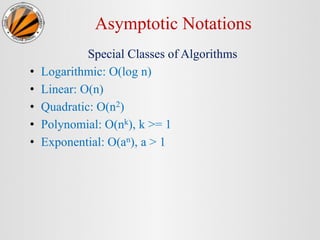
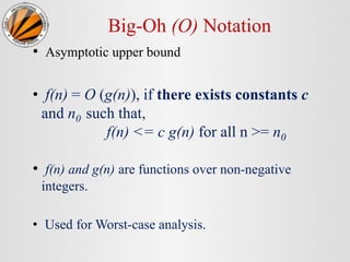
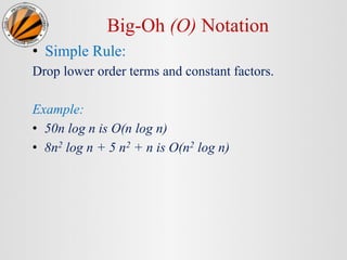
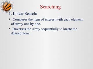
Data Structures & Algorithms
Topic : Asymptotic Notations & Complexity
Analysis
Contents
• Basic Terminology
• Complexity of Algorithm
• Asymptotic Notations
• Linear Search and Binary Search
• Review Questions
Basic Terminology
• Algorithm: is a finite step by step list of well-defined
instructions for solving a particular problem.
• Complexity of Algorithm: is a function which
gives running time and/or space requirement in terms of
the input size.
• Time and Space are two major measures of efficiency
of an algorithm.
Algorithm
Algorithm
Specification of Input
(e.g. any sequence of
natural numbers)
Specification of Output
as a function of Input
(e.g. sequence of sorted
natural numbers)
Characteristics of Good Algorithm
• Efficient
• Running Time
• Space used
• Efficiency as a function of input size
• Size of Input (5, 55555555555)
• Number of Data elements
Time-Space Tradeoff
• By increasing the amount of space for storing the
data, one may be able to reduce the time needed for
processing the data, or vice versa.
Complexity of Algorithm
• Time and Space used by the algorithm are two
main measures for efficiency of any algorithm M.
• Time is measured by counting the number of key
operations.
• Space is measured by counting the maximum of
memory needed by the algorithm.
• Complexity of Algorithm is a function
f(n) which gives running time and/or space
requirement of algorithm M in terms of the
size n of the input data.
• Worst Case: The maximum value of f(n) for
any possible input.
• Average Case: The expected or average value
of f(n).
• Best Case: Minimum possible value of f(n).
Rate of Growth
• The rate of growth of some standard functions
g(n) is:
log2n < n < nlog2n < n2 < n3 < 2n
Asymptotic Notations
• Goal: to simplify analysis of running time .
• Useful to identify how the running time of an
algorithm increases with the size of the input in the
limit.
Asymptotic Notations
Special Classes of Algorithms
• Logarithmic: O(log n)
• Linear: O(n)
• Quadratic: O(n2)
• Polynomial: O(nk), k >= 1
• Exponential: O(an), a > 1
Big-Oh (O) Notation
• Asymptotic upper bound
• f(n) = O (g(n)), if there exists constants c
and n0 such that,
f(n) <= c g(n) for all n >= n0
• f(n) and g(n) are functions over non-negative
integers.
• Used for Worst-case analysis.
Big-Oh (O) Notation
• Simple Rule:
Drop lower order terms and constant factors.
Example:
• 50n log n is O(n log n)
• 8n2 log n + 5 n2 + n is O(n2 log n)
Big-Omega (Ω) Notation
• Asymptotic lower bound
• f(n) = Ω (g(n)), if there exists constants c
and n0 such that,
c g(n) <= f(n) for all n >= n0
• Used to describe Best-case running time.
Big-Theta (Ө)Notation
• Asymptotic tight bound
• f(n) = Ө (g(n)), if there exists constants c1,
c2 and n0 such that,
c1 g(n) <= f(n) <= c2 g(n) for n >= n0
• f(n) = Ө (g(n)), iff f(n) = O(g(n)) and
f(n) = Ω (g(n))
Little-Oh (o) Notation
• Non-tight analogue of Big-Oh.
• f(n) = o (g(n)), if for every c there exists n0
such that,
f(n) < c g(n) for all n >= n0
• f(n) = o (g(n)), iff
f(n) = O (g(n)) and f(n) ≠ Ω (g(n))
• Used for comparisons of running times.
Questions
Review Questions
• When an algorithm is said to be better than the
other?
• Can an algorithm have different running times on
different machines?
• How the algorithm’ running time is dependent on
machines on which it is executed?
Review Questions
Find out the complexity:
function ()
{
if (condition)
{
for (i=0; i<n; i++) { // simple statements}
}
else
{
for (j=1; j<n; j++)
for (k=n; k>0; k--) {// simple statement}
}
}
Review Questions
Find out the complexity:
• void complex (int n)
{
for (int i=1; i*i<=n; i++)
for (int j=1; j*j<=n; j++)
{
cout<<” * ”;
}
}
Review Questions
Find out the complexity:
• void more_complex (int n)
{
for(int i=1; i<=n/3; i++)
{
for(int j=1; j<=n; j+=4)
{
cout<<” * ”;
break;
}
break;
}
}
Searching
Searching
1. Linear Search:
• Compares the item of interest with each element
of Array one by one.
• Traverses the Array sequentially to locate the
desired item.
Linear Search Algorithm
• LINEAR (DATA, N, ITEM, LOC)
1. [Insert ITEM at the end of DATA] Set Data [N]= ITEM.
2. [Initialize Counter] Set LOC=0.
3. [Search for ITEM.]
Repeat while DATA [LOC] != ITEM
Set LOC = LOC +1.
[End of loop.]
4. [Successful?] if LOC = N, then Print “ITEM not found”.
else return LOC.
5. Exit.
2. Binary Search
• BINARY ( DATA, LB, UB, ITEM, LOC )
1. [Initialize Segment Variables]
Set BEG = LB, END = UB and MID = INT ((BEG+END)/2).
2. Repeat Steps 3 and 4 while BEG < END and DATA [MID] != ITEM.
3. If ITEM < DATA[MID], then:
Set END = MID - 1.
Else:
Set BEG = MID + 1.
[End of if Structure.]
4. Set MID = INT ((BEG+END)/2).
[End of Step 2 Loop.]
5. If DATA [MID] = ITEM, then: Print “Item Found at ” LOC
Else:
Set LOC = NULL.
[End of if structure.]
6. Exit.
Limitations of Binary Search
• Although the complexity of Binary Search is
O (log n), it has some limitations:
1. the list must be sorted
2. one must have direct access to the middle element
in any sub-list.

2. Asymptotic Notations and Complexity Analysis.pptx

  • 1.
    Data Structures &Algorithms Topic : Asymptotic Notations & Complexity Analysis
  • 2.
    Contents • Basic Terminology •Complexity of Algorithm • Asymptotic Notations • Linear Search and Binary Search • Review Questions
  • 3.
    Basic Terminology • Algorithm:is a finite step by step list of well-defined instructions for solving a particular problem. • Complexity of Algorithm: is a function which gives running time and/or space requirement in terms of the input size. • Time and Space are two major measures of efficiency of an algorithm.
  • 4.
    Algorithm Algorithm Specification of Input (e.g.any sequence of natural numbers) Specification of Output as a function of Input (e.g. sequence of sorted natural numbers)
  • 5.
    Characteristics of GoodAlgorithm • Efficient • Running Time • Space used • Efficiency as a function of input size • Size of Input (5, 55555555555) • Number of Data elements
  • 6.
    Time-Space Tradeoff • Byincreasing the amount of space for storing the data, one may be able to reduce the time needed for processing the data, or vice versa.
  • 7.
    Complexity of Algorithm •Time and Space used by the algorithm are two main measures for efficiency of any algorithm M. • Time is measured by counting the number of key operations. • Space is measured by counting the maximum of memory needed by the algorithm.
  • 8.
    • Complexity ofAlgorithm is a function f(n) which gives running time and/or space requirement of algorithm M in terms of the size n of the input data. • Worst Case: The maximum value of f(n) for any possible input. • Average Case: The expected or average value of f(n). • Best Case: Minimum possible value of f(n).
  • 9.
    Rate of Growth •The rate of growth of some standard functions g(n) is: log2n < n < nlog2n < n2 < n3 < 2n
  • 10.
  • 11.
    Asymptotic Notations • Goal:to simplify analysis of running time . • Useful to identify how the running time of an algorithm increases with the size of the input in the limit.
  • 12.
    Asymptotic Notations Special Classesof Algorithms • Logarithmic: O(log n) • Linear: O(n) • Quadratic: O(n2) • Polynomial: O(nk), k >= 1 • Exponential: O(an), a > 1
  • 13.
    Big-Oh (O) Notation •Asymptotic upper bound • f(n) = O (g(n)), if there exists constants c and n0 such that, f(n) <= c g(n) for all n >= n0 • f(n) and g(n) are functions over non-negative integers. • Used for Worst-case analysis.
  • 14.
    Big-Oh (O) Notation •Simple Rule: Drop lower order terms and constant factors. Example: • 50n log n is O(n log n) • 8n2 log n + 5 n2 + n is O(n2 log n)
  • 15.
    Big-Omega (Ω) Notation •Asymptotic lower bound • f(n) = Ω (g(n)), if there exists constants c and n0 such that, c g(n) <= f(n) for all n >= n0 • Used to describe Best-case running time.
  • 16.
    Big-Theta (Ө)Notation • Asymptotictight bound • f(n) = Ө (g(n)), if there exists constants c1, c2 and n0 such that, c1 g(n) <= f(n) <= c2 g(n) for n >= n0 • f(n) = Ө (g(n)), iff f(n) = O(g(n)) and f(n) = Ω (g(n))
  • 17.
    Little-Oh (o) Notation •Non-tight analogue of Big-Oh. • f(n) = o (g(n)), if for every c there exists n0 such that, f(n) < c g(n) for all n >= n0 • f(n) = o (g(n)), iff f(n) = O (g(n)) and f(n) ≠ Ω (g(n)) • Used for comparisons of running times.
  • 18.
  • 19.
    Review Questions • Whenan algorithm is said to be better than the other? • Can an algorithm have different running times on different machines? • How the algorithm’ running time is dependent on machines on which it is executed?
  • 20.
    Review Questions Find outthe complexity: function () { if (condition) { for (i=0; i<n; i++) { // simple statements} } else { for (j=1; j<n; j++) for (k=n; k>0; k--) {// simple statement} } }
  • 21.
    Review Questions Find outthe complexity: • void complex (int n) { for (int i=1; i*i<=n; i++) for (int j=1; j*j<=n; j++) { cout<<” * ”; } }
  • 22.
    Review Questions Find outthe complexity: • void more_complex (int n) { for(int i=1; i<=n/3; i++) { for(int j=1; j<=n; j+=4) { cout<<” * ”; break; } break; } }
  • 23.
  • 24.
    Searching 1. Linear Search: •Compares the item of interest with each element of Array one by one. • Traverses the Array sequentially to locate the desired item.
  • 25.
    Linear Search Algorithm •LINEAR (DATA, N, ITEM, LOC) 1. [Insert ITEM at the end of DATA] Set Data [N]= ITEM. 2. [Initialize Counter] Set LOC=0. 3. [Search for ITEM.] Repeat while DATA [LOC] != ITEM Set LOC = LOC +1. [End of loop.] 4. [Successful?] if LOC = N, then Print “ITEM not found”. else return LOC. 5. Exit.
  • 26.
    2. Binary Search •BINARY ( DATA, LB, UB, ITEM, LOC ) 1. [Initialize Segment Variables] Set BEG = LB, END = UB and MID = INT ((BEG+END)/2). 2. Repeat Steps 3 and 4 while BEG < END and DATA [MID] != ITEM. 3. If ITEM < DATA[MID], then: Set END = MID - 1. Else: Set BEG = MID + 1. [End of if Structure.] 4. Set MID = INT ((BEG+END)/2). [End of Step 2 Loop.] 5. If DATA [MID] = ITEM, then: Print “Item Found at ” LOC Else: Set LOC = NULL. [End of if structure.] 6. Exit.
  • 27.
    Limitations of BinarySearch • Although the complexity of Binary Search is O (log n), it has some limitations: 1. the list must be sorted 2. one must have direct access to the middle element in any sub-list.

Editor's Notes

  • #3 목차 자바의 생성배경 자바를 사용하는 이유 과거, 현재, 미래의 자바 자바의 발전과정 버전별 JDK에 대한 설명 자바와 C++의 차이점 자바의 성능 자바 관련 산업(?)의 경향
  • #4 목차 자바의 생성배경 자바를 사용하는 이유 과거, 현재, 미래의 자바 자바의 발전과정 버전별 JDK에 대한 설명 자바와 C++의 차이점 자바의 성능 자바 관련 산업(?)의 경향
  • #5 목차 자바의 생성배경 자바를 사용하는 이유 과거, 현재, 미래의 자바 자바의 발전과정 버전별 JDK에 대한 설명 자바와 C++의 차이점 자바의 성능 자바 관련 산업(?)의 경향
  • #6 목차 자바의 생성배경 자바를 사용하는 이유 과거, 현재, 미래의 자바 자바의 발전과정 버전별 JDK에 대한 설명 자바와 C++의 차이점 자바의 성능 자바 관련 산업(?)의 경향
  • #7 목차 자바의 생성배경 자바를 사용하는 이유 과거, 현재, 미래의 자바 자바의 발전과정 버전별 JDK에 대한 설명 자바와 C++의 차이점 자바의 성능 자바 관련 산업(?)의 경향
  • #8 목차 자바의 생성배경 자바를 사용하는 이유 과거, 현재, 미래의 자바 자바의 발전과정 버전별 JDK에 대한 설명 자바와 C++의 차이점 자바의 성능 자바 관련 산업(?)의 경향
  • #9 목차 자바의 생성배경 자바를 사용하는 이유 과거, 현재, 미래의 자바 자바의 발전과정 버전별 JDK에 대한 설명 자바와 C++의 차이점 자바의 성능 자바 관련 산업(?)의 경향
  • #10 목차 자바의 생성배경 자바를 사용하는 이유 과거, 현재, 미래의 자바 자바의 발전과정 버전별 JDK에 대한 설명 자바와 C++의 차이점 자바의 성능 자바 관련 산업(?)의 경향
  • #11 목차 자바의 생성배경 자바를 사용하는 이유 과거, 현재, 미래의 자바 자바의 발전과정 버전별 JDK에 대한 설명 자바와 C++의 차이점 자바의 성능 자바 관련 산업(?)의 경향
  • #12 목차 자바의 생성배경 자바를 사용하는 이유 과거, 현재, 미래의 자바 자바의 발전과정 버전별 JDK에 대한 설명 자바와 C++의 차이점 자바의 성능 자바 관련 산업(?)의 경향
  • #13 목차 자바의 생성배경 자바를 사용하는 이유 과거, 현재, 미래의 자바 자바의 발전과정 버전별 JDK에 대한 설명 자바와 C++의 차이점 자바의 성능 자바 관련 산업(?)의 경향
  • #14 목차 자바의 생성배경 자바를 사용하는 이유 과거, 현재, 미래의 자바 자바의 발전과정 버전별 JDK에 대한 설명 자바와 C++의 차이점 자바의 성능 자바 관련 산업(?)의 경향
  • #15 목차 자바의 생성배경 자바를 사용하는 이유 과거, 현재, 미래의 자바 자바의 발전과정 버전별 JDK에 대한 설명 자바와 C++의 차이점 자바의 성능 자바 관련 산업(?)의 경향
  • #16 목차 자바의 생성배경 자바를 사용하는 이유 과거, 현재, 미래의 자바 자바의 발전과정 버전별 JDK에 대한 설명 자바와 C++의 차이점 자바의 성능 자바 관련 산업(?)의 경향
  • #17 목차 자바의 생성배경 자바를 사용하는 이유 과거, 현재, 미래의 자바 자바의 발전과정 버전별 JDK에 대한 설명 자바와 C++의 차이점 자바의 성능 자바 관련 산업(?)의 경향
  • #18 목차 자바의 생성배경 자바를 사용하는 이유 과거, 현재, 미래의 자바 자바의 발전과정 버전별 JDK에 대한 설명 자바와 C++의 차이점 자바의 성능 자바 관련 산업(?)의 경향
  • #19 목차 자바의 생성배경 자바를 사용하는 이유 과거, 현재, 미래의 자바 자바의 발전과정 버전별 JDK에 대한 설명 자바와 C++의 차이점 자바의 성능 자바 관련 산업(?)의 경향
  • #20 목차 자바의 생성배경 자바를 사용하는 이유 과거, 현재, 미래의 자바 자바의 발전과정 버전별 JDK에 대한 설명 자바와 C++의 차이점 자바의 성능 자바 관련 산업(?)의 경향
  • #22 목차 자바의 생성배경 자바를 사용하는 이유 과거, 현재, 미래의 자바 자바의 발전과정 버전별 JDK에 대한 설명 자바와 C++의 차이점 자바의 성능 자바 관련 산업(?)의 경향
  • #23 O(N^2)
  • #24 O(N^2)
  • #25 O(N^2)
  • #26 목차 자바의 생성배경 자바를 사용하는 이유 과거, 현재, 미래의 자바 자바의 발전과정 버전별 JDK에 대한 설명 자바와 C++의 차이점 자바의 성능 자바 관련 산업(?)의 경향
  • #27 목차 자바의 생성배경 자바를 사용하는 이유 과거, 현재, 미래의 자바 자바의 발전과정 버전별 JDK에 대한 설명 자바와 C++의 차이점 자바의 성능 자바 관련 산업(?)의 경향
  • #28 목차 자바의 생성배경 자바를 사용하는 이유 과거, 현재, 미래의 자바 자바의 발전과정 버전별 JDK에 대한 설명 자바와 C++의 차이점 자바의 성능 자바 관련 산업(?)의 경향
  • #29 목차 자바의 생성배경 자바를 사용하는 이유 과거, 현재, 미래의 자바 자바의 발전과정 버전별 JDK에 대한 설명 자바와 C++의 차이점 자바의 성능 자바 관련 산업(?)의 경향
  • #30 목차 자바의 생성배경 자바를 사용하는 이유 과거, 현재, 미래의 자바 자바의 발전과정 버전별 JDK에 대한 설명 자바와 C++의 차이점 자바의 성능 자바 관련 산업(?)의 경향