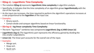
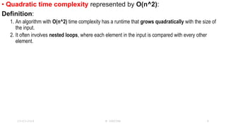
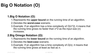
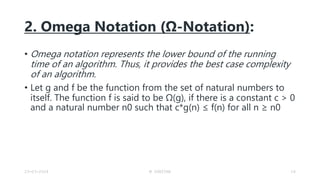
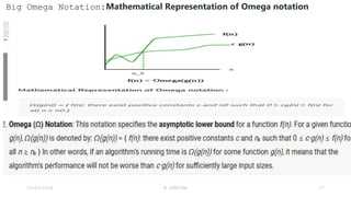
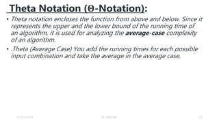
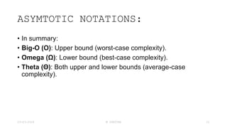
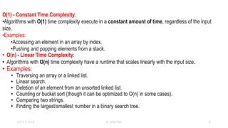
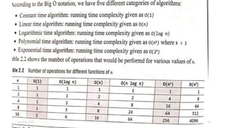
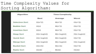
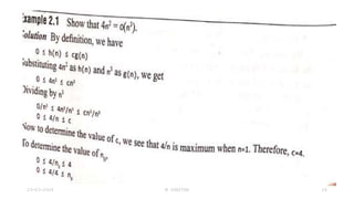
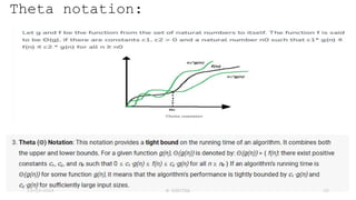
1. The document discusses various asymptotic notations used to analyze algorithm efficiency such as Big O, Omega, and Theta notations. 2. It provides examples of time complexity for common algorithms like searching, sorting, etc. 3. The asymptotic notations help understand how an algorithm's running time scales with increasing input size.

1. UNIT –I
ASYMTOTIC NOTATIONS
• M.SUNITHA
23-03-2024 M SUNITHA 1

2. Algorithm Analysis
• Analysis of efficiency of an algorithm can be performed at two different stages, before
implementation and after implementation, as
• A priori analysis − This is defined as theoretical analysis of an algorithm. Efficiency of algorithm is
measured by assuming that all other factors e.g. speed of processor, are constant and have no
effect on implementation.
• A posterior analysis − This is defined as empirical analysis of an algorithm. The chosen algorithm
is implemented using programming language. Next the chosen algorithm is executed on target
computer machine. In this analysis, actual statistics like running time and space needed are
collected.
• Algorithm analysis is dealt with the execution or running time of various operations involved.
Running time of an operation can be defined as number of computer instructions executed per
operation.
23-03-2024 M SUNITHA 2

3. Algorithm Complexity:
• Suppose X is treated as an algorithm and N is treated as the size of input data, the
time and space implemented by the Algorithm X are the two main factors which
determine the efficiency of X.
• Time Factor − The time is calculated or measured by counting the number of key
operations such as comparisons in sorting algorithm.
• Space Factor − The space is calculated or measured by counting the maximum
memory space required by the algorithm.
• The complexity of an algorithm f(N) provides the running time and / or storage
space needed by the algorithm with respect of N as the size of input data.
23-03-2024 M SUNITHA 3

4. Space Complexity
• Space complexity of an algorithm represents the amount of memory space needed the
algorithm in its life cycle.
• Space needed by an algorithm is equal to the sum of the following two components
1.A fixed part that is a space required to store certain data and variables (i.e. simple variables and
constants, program size etc.), that are not dependent of the size of the problem.
2.A variable part is a space required by variables, whose size is totally dependent on the size of
the problem. For example, recursion stack space, dynamic memory allocation etc.
23-03-2024 M SUNITHA 4

5. Algoritham:
SUM(P, Q)
Step 1 – START
Step 2 –
R ← P + Q + 10
Step 3 - Stop
• Time Complexity of an algorithm is the representation of the amount of time required by the algorithm to execute to
completion. Time requirements can be denoted or defined as a numerical function t(N), where t(N) can be
measured as the number of steps, provided each step takes constant time.
• For example, in case of addition of two n-bit integers, N steps are taken. Consequently, the total computational time
is t(N) = c*n, where c is the time consumed for addition of two bits. Here, we observe that t(N) grows linearly as
input size increases.
• Space Complexity:
• Here we have three variables P, Q and R and one constant. Hence S(p) = 1+3. Now space is dependent on data
types of given constant types and variables and it will be multiplied accordingly.
23-03-2024 M SUNITHA 5

6. O(1) - Constant Time Complexity:
•Algorithms with O(1) time complexity execute in a constant amount of time, regardless of the input
size.
•Examples:
•Accessing an element in an array by index.
•Pushing and popping elements from a stack.
• O(n) - Linear Time Complexity:
• Algorithms with O(n) time complexity have a runtime that scales linearly with the input size.
• Examples:
• Traversing an array or a linked list.
• Linear search.
• Deletion of an element from an unsorted linked list.
• Counting or bucket sort (though it can be optimized to O(n) in some cases).
• Comparing two strings.
• Finding the largest/smallest number in a binary search tree.
23-03-2024 M SUNITHA 6

7. • O(log n) - Logarithmic Time Complexity:
• The notation O(log n) represents logarithmic time complexity in algorithm analysis.
• Specifically, it indicates that the time complexity of an algorithm grows logarithmically with the
size of the input (n).
• As the input size increases, the time required to perform the algorithm’s operations increases at
a rate proportional to the logarithm of the input size.
• Examples:
• Binary search..
• Certain divide-and-conquer algorithms based on linear functionality.
• O(n log n) - log-linear complexity Time Complexity:
• The term “log-linear” combines two components:Logarithmic (log n) AND Linear (n)
• Logarithmic (log n) :The logarithmic part represents the efficiency gained by dividing the
into smaller subproblems.
• Linear (n): The linear part accounts for the overall size of the input.
• Examples:
• Merge sort.
• Heap sort.
• Quick sort.
23-03-2024 M SUNITHA 7

8. • Quadratic time complexity represented by O(n^2):
Definition:
1. An algorithm with O(n^2) time complexity has a runtime that grows quadratically with the size of
the input.
2. It often involves nested loops, where each element in the input is compared with every other
element.
23-03-2024 M SUNITHA 8

9. Asymptotic notations
asymptotic notations, which are essential for analyzing the efficiency and
performance of algorithms. These notations help us understand how an
algorithm’s running time or space requirements change as the input size
grows.
23-03-2024 M SUNITHA 9

10. Asymptotic Notations
1.Big O Notation (O)
2.Big Omega Notation (Ω)
3.Big Theta Notation (Θ)
4.Little O notation
5.Little omega notation
23-03-2024 M SUNITHA 10

11. Big O Notation (O)
1.Big O Notation (O):
1.Represents the upper bound on the running time of an algorithm.
2.Denotes the worst-case scenario.
3.Example: If an algorithm has a time complexity of O(n^2), it means that
the running time grows no faster than n^2 as the input size (n)
increases.
2.Big Omega Notation (Ω):
1.Represents the lower bound on the running time of an algorithm.
2.Denotes the best-case scenario.
3.Example: If an algorithm has a time complexity of Ω(n), it means that
the running time grows at least as fast as n.
23-03-2024 M SUNITHA 11

12. Asymtotic notations:
3.Big Theta Notation (Θ):
1. Represents both the upper and lower bounds on the running time of an
algorithm.
2. Denotes the average-case scenario.
3. Example: If an algorithm has a time complexity of Θ(n), it means that the
running time grows exactly as fast as n.
4.Little o Notation (o):
1. Definition: Let f(n) and g(n) be functions that map positive integers to
positive real numbers. We say that f(n) is o(g(n)) (or f(n) = o(g(n))), if for any
real constant c > 0, there exists an integer constant n₀ ≥ 1 such that 0 ≤ f(n) <
c * g(n).
2. Interpretation: Little o provides a loose upper bound on the growth
of f(n) compared to g(n). It means that f(n) grows strictly slower than g(n).
3. Example: If f(n) = 7n + 8, then 7n + 8 = o(n²) because the
ratio f(n)/g(n) approaches zero as n increases.
23-03-2024 M SUNITHA 12

13. Asymtotic Notations:
5.Small Omega Notation (ω):
Definition: Let f(n) and g(n) be functions that map positive integers to positive real numbers. We say
that f(n) is ω(g(n)) (or f(n) = ω(g(n))), if for any real constant c > 0, there exists an integer constant n₀
≥ 1 such that f(n) > c * g(n) for every integer n ≥ n₀.
Interpretation: Small ω provides a loose lower bound on the growth of f(n) compared to g(n). It
means that f(n) grows strictly faster than g(n).
Example: If f(n) = 4n + 6, then 4n + 6 = ω(1) because the ratio f(n)/g(n) approaches infinity
as n increases.
NOTE:
Little o represents a loose upper bound.
Small ω represents a loose lower bound.
These notations help us understand the behavior of algorithms beyond the tight bounds
provided by Big O and Big Ω. They are useful for analyzing more subtle differences in
growth rates.
23-03-2024 M SUNITHA 13

14. Big-O Notation (O-notation):
23-03-2024 M SUNITHA 14

15. BIG O NOTATION:
23-03-2024 M SUNITHA 15

16. 2. Omega Notation (Ω-Notation):
• Omega notation represents the lower bound of the running
time of an algorithm. Thus, it provides the best case complexity
of an algorithm.
• Let g and f be the function from the set of natural numbers to
itself. The function f is said to be Ω(g), if there is a constant c > 0
and a natural number n0 such that c*g(n) ≤ f(n) for all n ≥ n0
23-03-2024 M SUNITHA 16

17. Big Omega Notation:Mathematical Representation of Omega notation
23-03-2024 M SUNITHA 17

18. 23-03-2024 M SUNITHA 18

19. Theta Notation (Θ-Notation):
• Theta notation encloses the function from above and below. Since it
represents the upper and the lower bound of the running time of
an algorithm, it is used for analyzing the average-case complexity
of an algorithm.
• .Theta (Average Case) You add the running times for each possible
input combination and take the average in the average case.
23-03-2024 M SUNITHA 19

20. Theta notation:
23-03-2024 M SUNITHA 20

21. ASYMTOTIC NOTATIONS:
• In summary:
• Big-O (O): Upper bound (worst-case complexity).
• Omega (Ω): Lower bound (best-case complexity).
• Theta (Θ): Both upper and lower bounds (average-case
complexity).
23-03-2024 M SUNITHA 21

22. Time Complexity Values for
Sorting Algoritham:
23-03-2024 M SUNITHA 22

23. 23-03-2024 M SUNITHA 23

24. 23-03-2024 M SUNITHA 24