11 rocket dyanmics.pdf

Rocket Vehicle Dynamics
11
CHAPTER OUTLINE
11.1 Introduction ................................................................................................................................619
11.2 Equations of motion.....................................................................................................................620
11.3 The thrust equation .....................................................................................................................622
11.4 Rocket performance ....................................................................................................................624
11.5 Restricted staging in field-free space ...........................................................................................630
11.6 Optimal staging...........................................................................................................................640
Lagrange multiplier ...........................................................................................................640
Problems.............................................................................................................................................648
Section 11.4 .......................................................................................................................................648
Section 11.5 .......................................................................................................................................648
Section 11.6 .......................................................................................................................................649
11.1 Introduction
In previous chapters, we have made frequent reference to delta-v maneuvers of spacecraft. These require a
propulsion system of some sort whose job is to throw vehicle mass (in the form of propellants) overboard.
Newton’s balance of momentum principle dictates that when mass is ejected from a system in one di-
rection, the mass left behind must acquire a velocity in the opposite direction. The familiar and oft-quoted
example is the rapid release of air from an inflated toy balloon.Another is that of a diver leaping off a small
boat at rest in the water, causing the boat to acquire a motion of its own. The unfortunate astronaut who
becomes separated from his ship in the vacuum of space cannot with any amount of flailing of arms and
legs “swim” back to safety. If he has tools or other expendable objects of equipment, accurately throwing
them in the direction opposite to his spacecraft may do the trick. Spewing compressed gas from a tank
attached to his back through a nozzle pointed away from the spacecraft would be a better solution.
The purpose of a rocket motor is to use the chemical energy of solid or liquid propellants to steadily
and rapidly produce a large quantity of hot high-pressure gas, which is then expanded and accelerated
through a nozzle. This large mass of combustion products flowing out of the nozzle at supersonic speed
possesses a lot of momentum and, leaving the vehicle behind, causes the vehicle itself to acquire a
momentum in the opposite direction. This is represented as the action of the force we know as thrust.
The design and analysis of rocket propulsion systems is well beyond our scope.
This chapter contains a necessarily brief introduction to some of the fundamentals of rocket vehicle
dynamics. The equations of motion of a launch vehicle in a gravity turn trajectory are presented first.
This is followed by a simple development of the thrust equation, which brings in the concept of specific
CHAPTER
Orbital Mechanics for Engineering Students. http://dx.doi.org/10.1016/B978-0-08-097747-8.00011-6
Copyright Ó 2014 Elsevier Ltd. All rights reserved.
619

impulse. The thrust equation and the equations of motion are then combined to produce the rocket
equation, which relates delta-v to propellant expenditure and specific impulse. The sounding rocket
provides an important but relatively simple application of the concepts introduced to this point. After a
computer simulation of a gravity turn trajectory, the chapter concludes with an elementary consid-
eration of multistage launch vehicles.
Those seeking a more detailed introduction to the subject of rockets and rocket performance will
find the texts by Wiesel (1997) and Hale (1994), as well as references cited therein, useful.
11.2 Equations of motion
Figure 11.1 illustrates the trajectory of a satellite launch vehicle and the forces acting on it during the
powered ascent. Rockets at the base of the booster produce the thrust T, which acts along the vehicle’s
axis in the direction of the velocity vector v. The aerodynamic drag force D is directed opposite to the
velocity, as shown. Its magnitude is given by
D ¼ qACD (11.1)
where q ¼ 1
2rv2 is the dynamic pressure, in which r is the density of the atmosphere and v is the speed,
that is, the magnitude of v. A is the frontal area of thevehicleand CD is the coefficient of drag. CD depends
on the speed and the external geometry of the rocket. The force of gravity on the booster is mg, where m is
its mass and g is the local gravitational acceleration, pointing toward the center of the earth. As discussed
in Section 1.3, at any point of the trajectory, the velocity v defines the direction of the unit tangent ^
ut to
the path. The unit normal ^
un is perpendicular to v and points toward the center of curvature C. The
distance of point C from the path is r (not to be confused with density). r is the radius of curvature.
In Figure 11.1, the vehicle and its flight path are shown relative to the earth. In the interest of
simplicity we will ignore the earth’s spin and write the equations of motion relative to a nonrotating
earth. The small acceleration terms required to account for the earth’s rotation can be added for a more
T
D
g
v
C
ût
ûn
Trajectory's center of curvature
Trajectory
Local horizon
To earth's center
FIGURE 11.1
Launch vehicle boost trajectory. g is the flight path angle.
620 CHAPTER 11 Rocket Vehicle Dynamics

refined analysis. Let us resolve Newton’s second law, Fnet ¼ ma, into components along the path di-
rections ^
ut and ^
un. Recall from Section 1.3 that the acceleration along the path is
at ¼
dv
dt
(11.2)
and the normal acceleration is an ¼ v2
/r (where r is the radius of curvature). It was shown in Example
1.8 (Eqn (1.37)) that for flight over a flat surface, v/r ¼ dg/dt, in which case the normal acceleration
can be expressed in terms of the flight path angle as
an ¼ v
dg
dt
To account for the curvature of the earth, as was done in Section 1.7, one can use polar coordinates
with origin at the earth’s center to show that a term must be added to this expression, so that it becomes
an ¼ v
dg
dt
þ
v2
RE þ h
cos g (11.3)
where RE is the radius of the earth and h (instead of z as in previous chapters) is the altitude of the
rocket. Thus, in the direction of ^
ut, Newton’s second law requires
T D mg sin g ¼ mat (11.4)
whereas in the ^
un direction
mg cos g ¼ man (11.5)
After substituting Eqns (11.2) and (11.3), the latter two expressions may be written:
dv
dt
¼
T
m

D
m
g sin g (11.6)
v
dg
dt
¼

g
v2
RE þ h

cos g (11.7)
To these we must add the equations for downrange distance x and altitude h,
dx
dt
¼
RE
RE þ h
v cos g
dh
dt
¼ v sin g (11.8)
Recall that the variation of g with altitude is given by Eqn (1.36). Numerical methods must be used
to solve Eqns (11.6), (11.7) and (11.8). To do so, one must account for the variation of the thrust,
booster mass, atmospheric density, the drag coefficient, and the acceleration of gravity. Of course, the
vehicle mass continuously decreases as propellants are consumed to produce the thrust, which we shall
discuss in the following section.
The free body diagram in Figure 11.1 does not include a lifting force, which, if the vehicle were an
airplane, would act normal to the velocity vector. Launch vehicles are designed to be strong in
lengthwise compression, like a column. To save weight they are, unlike an airplane, made relatively
weak in bending, shear, and torsion, which are the kinds of loads induced by lifting surfaces.
Transverse lifting loads are held closely to zero during powered ascent through the atmosphere by
maintaining zero angle of attack, that is, by keeping the axis of the booster aligned with its velocity
11.2 Equations of motion 621

vector (the relative wind). Pitching maneuvers are done early in the launch, soon after the rocket clears
the launch tower, when its speed is still low. At the high speeds acquired within a minute or so after
launch, the slightest angle of attack can produce destructive transverse loads in the vehicle. The Space
Shuttle orbiter had wings so that it could act as a glider after reentry into the atmosphere. However, the
launch configuration of the orbiter was such that its wings were at the zero lift angle of attack
throughout the ascent.
Satellite launch vehicles take off vertically and, at injection into orbit, must be flying parallel to the
earth’s surface. During the initial phase of the ascent, the rocket builds up speed on a nearly vertical
trajectory taking it above the dense lower layers of the atmosphere. While it transitions to the thinner
upper atmosphere, the trajectory bends over, trading vertical speed for horizontal speed so that the
rocket can achieve orbital perigee velocity at burnout. The gradual transition from vertical to hori-
zontal flight, illustrated in Figure 11.1, is caused by the force of gravity, and it is called a gravity turn
trajectory.
At liftoff the rocket is vertical, and the flight path angle g is 90. After clearing the tower and
gaining speed, vernier thrusters or gimbaling of the main engines produce a small, programmed
pitchover, establishing an initial flight path angle go, slightly less than 90. Thereafter, g will continue
to decrease at a rate dictated by Eqn (11.7). (For example, if g ¼ 85, v ¼ 110 m/s (250 mph), and
h ¼ 2 km, then dg/dt ¼ 0.44 deg/s.) As the speed v of the vehicle increases, the coefficient of cos g in
Eqn (11.7) decreases, which means the rate of change of the flight path angle becomes increasingly
smaller, tending toward zero as the booster approaches orbital speed, vcircular orbit ¼
ffiffiffiffiffiffiffiffiffiffiffiffiffiffiffiffiffiffi
gðR þ hÞ
p
.
Ideally, the vehicle is flying horizontally (g ¼ 0) at that point.
The gravity turn trajectory is just one example of a practical trajectory, tailored for satellite
boosters. On the other hand, sounding rockets fly straight up from launch through burnout. Rocket-
powered guided missiles must execute high-speed pitch and yaw maneuvers as they careen toward
moving targets and require a rugged structure to withstand the accompanying side loads.
11.3 The thrust equation
To discuss rocket performance requires an expression for the thrust T in Eqn (11.6). It can be ob-
tained by a simple one-dimensional momentum analysis. Figure 11.2(a) shows a system consisting of
a rocket and its propellants. The exterior of the rocket is surrounded by the static pressure pa of the
atmosphere everywhere except at the rocket nozzle exit where the pressure is pe. pe acts over the
nozzle exit area Ae. The value of pe depends on the design of the nozzle. For simplicity, we assume
that no other forces act on the system. At time t the mass of the system is m and the absolute velocity
in its axial direction is v. The propellants combine chemically in the rocket’s combustion chamber,
and during the small time interval Dt a small mass Dm of combustion products is forced out of the
nozzle, to the left. Because of this expulsion, the velocity of the rocket changes by the small amount
Dv, to the right. The absolute velocity of Dm is ve, assumed to be to the left. According to Newton’s
second law of motion,
ðmomentum of the system at t þ DtÞ ðmomentum of the system at tÞ ¼ net external impulse
or
h
ðm DmÞðv þ DvÞ^
i þ Dm

ve
^
i
i
mv^
i ¼ ðpe paÞAeDt^
i (11.9)

Let _
me (a positive quantity) be the rate at which exhaust mass flows across the nozzle exit plane.
The mass m of the rocket decreases at the rate dm/dt, and conservation of mass requires the decrease of
mass to equal the mass flow rate out of the nozzle. Thus,
dm
dt
¼ _
me (11.10)
Assuming _
me is constant, the vehicle mass as a function of time (from t ¼ 0) may therefore be written
mðtÞ ¼ mo _
met (11.11)
where mo is the initial mass of the vehicle. Since Dm is the mass that flows out in the time interval Dt,
we have
Dm ¼ _
meDt (11.12)
Let us substitute this expression into Eqn (11.9) to obtain
h
ðm _
meDtÞðv þ DvÞ^
i þ _
meDt

ve
^
i
i
mv^
i ¼ ðpe paÞAeDt^
i
Collecting terms, we get
mDv^
i _
meDtðve þ vÞ^
i _
meDtDv^
i ¼ ðpe paÞAeDt^
i
Dividing through by Dt, taking the limit as Dt/0, and canceling the common unit vector leads to
m
dv
dt
_
meca ¼ ðpe paÞAe (11.13)
where ca is the speed of the exhaust relative to the rocket,
ca ¼ ve þ v (11.14)
Rearranging terms, Eqn (11.13) may be written
_
meca þ ðpe paÞAe ¼ m
dv
dt
(11.15)
(a) (b)
FIGURE 11.2
(a) System of rocket and propellant at time t. (b) The system an instant later, after ejection of a small element Dm
of combustion products.
11.3 The thrust equation 623

The left-hand side of this equation is the unbalanced force responsible for the acceleration dv/dt of the
system in Figure 11.2. This unbalanced force is the thrust T,
T ¼ _
meca þ ðpe paÞAe (11.16)
where _
meca is the jet thrust and (pe pa)Ae is the pressure thrust. We can write Eqn (11.16) as
T ¼ _
me

ca þ
ðpe paÞAe
_
me

(11.17)
The term in brackets is called the effective exhaust velocity c,
c ¼ ca þ
ðpe paÞAe
_
me
(11.18)
In terms of the effective exhaust velocity, the thrust may be expressed simply as
T ¼ _
mec (11.19)
The specific impulse Isp is defined as the thrust per sea level weight rate (per second) of propellant
consumption, that is,
Isp ¼
T
_
mego
(11.20)
where g0 is the standard sea level acceleration of gravity. The unit of specific impulse is force O
(force/second) or seconds. Together, Eqns (11.19) and (11.20) imply that
c ¼ Ispgo (11.21)
Obviously, one can infer the jet velocity directly from the specific impulse. Specific impulse is an
important performance parameter for a given rocket engine and propellant combination. However,
large specific impulse equates to large thrust only if the mass flow rate is large, which is true of
chemical rocket engines. The specific impulse of chemical rockets typically lies in the range 200–300 s
for solid fuels and 250–450 s for liquid fuels. Ion propulsion systems have very high specific impulse
(104
s), but their very low mass flow rates produce much smaller thrust than chemical rockets.
11.4 Rocket performance
From Eqns (11.10) and (11.20) we have
T ¼ Ispgo
dm
dt
(11.22)
or
dm
dt
¼
T
Ispgo

If the thrust and specific impulse are constant, then the integral of this expression over the burn time Dt is
Dm ¼
T
Ispgo
Dt
from which we obtain
Dt ¼
Ispgo
T
mo mf ¼
Ispgo
T
mo

1
mf
mo

(11.23)
where mo and mf are the mass of the vehicle at the beginning and end of the burn, respectively. The
mass ratio is defined as the ratio of the initial mass to final mass,
n ¼
mo
mf
(11.24)
Clearly, the mass ratio is always greater than unity. In terms of the initial mass ratio, Eqn (11.23) may
be written
Dt ¼
n 1
n
Isp
T=ðmogoÞ
(11.25)
T/(mgo) is the thrust-to-weight ratio. The thrust-to-weight ratio for a launch vehicle at liftoff is typi-
cally in the range 1.3–2.
Substituting Eqn (11.22) into Eqn (11.6), we get
dv
dt
¼ Ispgo
dm=dt
m

D
m
g sin g
Integrating with respect to time, from to to tf, yields
Dv ¼ Ispgoln
mo
mf
DvD DvG (11.26)
where the drag loss DvD and the gravity loss DvG are given by the integrals
DvD ¼
Ztf
to
D
m
dt DvG ¼
Ztf
to
g sin gdt (11.27)
Since the drag D, acceleration of gravity g, and flight path angle g are unknown functions of time,
these integrals cannot be computed. (Equation (11.6) through Eqn (11.8), together with Eqn (11.3),
must be solved numerically to obtain v(t) and g(t); but then Dv would follow from those results.)
Equation (11.26) can be used for rough estimates where previous data and experience provide a basis
for choosing conservative values of DvD and DvG. Obviously, if drag can be neglected, then DvD ¼ 0.
This would be a good approximation for the last stage of a satellite booster, for which it can also be said
that DvG ¼ 0, since gy0 when the satellite is injected into orbit.
Sounding rockets are launched vertically and fly straight up to their maximum altitude before
falling back to earth, usually by parachute. Their purpose is to measure remote portions of the earth’s
atmosphere. (“Sound” in this context means to measure or investigate.) If for a sounding rocket
g ¼ 90, then DvGzgoðtf t0Þ, since g is within 90% of go up to 300 km altitude.
11.4 Rocket performance 625

EXAMPLE 11.1
A sounding rocket of initial mass mo and mass mf after all propellant is consumed is launched vertically (g ¼ 90).
The propellant mass flow rate _
me is constant.
(a) Neglecting drag and the variation of gravity with altitude, calculate the maximum height h attained by the
rocket.
(b) For what flow rate is the greatest altitude reached?
Solution
The vehicle mass as a function of time, up to burnout, is
m ¼ mo _
met (a)
At burnout, m ¼ mf, so the burnout time tbo is
tbo ¼
mo mf
_
me
(b)
The drag loss is assumed zero, and the gravity loss is
DvG ¼
Z
tbo
0
go sinð90
Þdt ¼ got
Recalling that Ispgo ¼ c and using Eqn (a), it follows from Eqn (11.26) that, up to burnout, the velocity as a
function of time is
v ¼ c ln
mo
mo _
met
got (c)
Since dh/dt ¼ v, the altitude as a function of time is
h ¼
Zt
0
vdt ¼
Zt
0

c ln
mo
mo _
met
got

dt ¼
c
_
me

ðmo _
metÞ ln
mo _
met
mo
þ _
met

1
2
got2
(d)
The height at burnout hbo is found by substituting Eqn (b) into this expression,
hbo ¼
c
_
me

mf ln
mf
mo
þ mo mf

1
2

mo mf
_
me
2
go (e)
Likewise, the burnout velocity is obtained by substituting Eqn (b) into Eqn (c),
vbo ¼ c ln
mo
mf

go
_
me
ðmo mf Þ (f)
After burnout, the rocket coasts upward with the constant downward acceleration of gravity,
v ¼ vbo goðt tboÞ
h ¼ hbo þ vboðt tboÞ
1
2
goðt tboÞ2
Substituting Eqns (b), (e), and (f) into these expressions yields, for t tbo,
v ¼ c ln
mo
mf
got
h ¼
c
_
me

mo ln
mf
mo
þ mo mf

þ ct ln
mo
mf

1
2
g0t2
(g)

The maximum height hmax is reached when v ¼ 0,
c ln
mo
mf
gotmax ¼ 0 0 tmax ¼
c
go
ln
mo
mf
(h)
Substituting tmax into Eqn (g) leads to our result,
hmax ¼
1
2
c2
go
ln2
n
cmo
_
me
n lnn ðn 1Þ
n
(i)
where n is the mass ratio (n 1). Since n ln n is greater than n 1, it follows that the second term in this
expression is positive. Hence, hmax can be increased by increasing the mass flow rate _
me. In fact,
the greatest height is achieved when _
me/N
In that extreme, all the propellant is expended at once, like a mortar shell.
EXAMPLE 11.2
The data for a single-stage rocket are as follows:
Launch mass: mo ¼ 68,000 kg
Mass ratio: n ¼ 15
Specific impulse: Isp ¼ 390 s
Thrust: T ¼ 933.91 kN
It is launched into a vertical trajectory, like a sounding rocket. Neglecting drag and assuming that the gravitational
acceleration is constant at its sea level value go ¼ 9.81 m/s2
, calculate
(a) The time until burnout.
(b) The burnout altitude.
(c) The burnout velocity.
(d) The maximum altitude reached.
Solution
(a) From Example 11.1(b), the burnout time tbo is
tbo ¼
mo mf
_
me
(a)
The burnout mass mf is obtained from Eqn (11.24),
mf ¼
mo
n
¼
68;000
15
¼ 4533:3 kg (b)
The propellant mass flow rate _
me is given by Eqn (11.20),
_
me ¼
T
Ispgo
¼
933;913
390$9:81
¼ 244:10 kg=s (c)
Substituting Eqns (b), (c), and mo ¼ 68,000 kg into Eqn (a) yields the burnout time,
tbo ¼
68;000 4533:3
244:10
¼ 260:0 s
(b) The burnout altitude is given by Example 11.1(e),
hbo ¼
c
_
me

mf ln
mf
mo
þ mo mf

1
2

mo mf
_
me
2
go (d)

The exhaust velocity c is found in Eqn (11.21),
c ¼ Ispgo ¼ 390$9:81 ¼ 3825:9 m=s (e)
Substituting Eqns (b), (c), and (e), along with mo ¼ 68,000 kg and go ¼ 9.81 m/s2
, into Eqn (e), we get
hbo ¼
3825:9
244:1

4533:3 ln
4533:3
68;000
þ 68; 000 4533:3

1
2

68;000 4533:3
244:1
2
$ 9:81
hbo ¼ 470:74 km
(c) From Example 11.1(f), we find
vbo ¼ c ln
mo
mf

go
_
me
ðmo mf Þ ¼ 3825:9 ln
68;000
4533:3

9:81
244:1
ð68;000 4533:3Þ
vbo ¼ 7:810 km=s
(d) To find hmax, where the speed of the rocket falls to zero, we use Example 11.1(i),
hmax ¼
1
2
c2
go
ln2
n
cmo
_
me
nlnn ðn 1Þ
n
¼
1
2
3825:92
9:81
ln2
15
3825:9$68;000
244:1
15ln15 ð15 1Þ
15
hmax ¼ 3579:7 km
Notice that the rocket coasts to a height more than seven times the burnout altitude.
We can employ the integration schemes introduced in Section 1.8 to solve Eqn (11.6) through Eqn
(11.8) numerically. This permits a more accurate accounting of the effects of gravity and drag. It also
yields the trajectory.
EXAMPLE 11.3
The rocket in Example 11.2 has a diameter of 5 m. It is to be launched on a gravity turn trajectory. Pitchover begins
at an altitude of 130 m with an initial flight path angle go of 89.85. What are the altitude h and speed v of the
rocket at burnout (tbo ¼ 260 s)? What are the velocity losses due to drag and gravity (cf. Eqn (11.27))?
Solution
The MATLAB program Example_11_03.m in Appendix D.40 finds the speed v, the flight path angle g, the altitude
h, and the downrange distance x as a function of time. It does so by using the ordinary differential equation solver
rkf_45.m (Appendix D.4) to numerically integrate Eqn (11.6) through Eqn (11.8), namely
dv
dt
¼
T
m

D
m
g sin g (a)
dg
dt
¼
1
v

g
v2
RE þ h

cos g (b)
dh
dt
¼ v sin g (c)
dx
dt
¼
RE
RE þ h
v cos g (d)

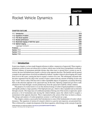
The variable mass m is given in terms of the initial mass mo ¼ 68,000 kg and the constant mass flow rate _
me by
Eqn (11.11),
m ¼ mo _
met (e)
The thrust T ¼ 933.913 kN is assumed constant, and _
me is obtained from T and the specific impulse
Isp ¼ 390 by means of Eqn (11.20),
_
me ¼
T
Ispgo
(f)
The drag force D in Eqn (a) is given by Eqn (11.1),
D ¼
1
2
rv2
ACD (g)
The drag coefficient is assumed to have the constant value CD ¼ 0.5. The frontal area A ¼ pd 2
/4 is found from
the rocket diameter d ¼ 5 m. The atmospheric density profile is assumed exponential,
r ¼ roeh=ho
(h)
where ro ¼ 1.225 kg/m3
is the sea level atmospheric density and ho ¼ 7.5 km is the scale height of the atmo-
sphere. (The scale height is the altitude at which the density of the atmosphere is about 37% of its sea level value.)
Finally, the acceleration of gravity varies with altitude h according to Eqn (1.36),
g ¼
go
ð1 þ h=REÞ2

RE ¼ 6378 km; go ¼ 9:81 m=s2

(i)
The drag loss and gravity loss are found by numerically integrating Eqn (11.27).
Between liftoff and pitchover, the flight path angle g is held at 90. Pitchover begins at the altitude
hp ¼ 130 m with the flight path angle set at go ¼ 89.85.
For the input data described above, the output of Example_11_03.m is as follows. The solution is very sen-
sitive to the values of hp and go.
Thus, at burnout
Altitude ¼ 133:2 km
Speed ¼ 8:621 km=s
The speed losses are
Due to drag : 0:2982 km=s
Due to gravity : 1:441 km=s
Figure 11.3 shows the gravity turn trajectory.

11.5 Restricted staging in field-free space
In field-free space, we neglect drag and gravitational attraction. In that case, Eqn (11.26) becomes
Dv ¼ Ispgo ln
mo
mf
(11.28)
This is at best a poor approximation for high-thrust rockets, but it will suffice to shed some light on the
rocket staging problem. Observe that we can solve this equation for the mass ratio to obtain
mo
mf
¼ e
Dv
Ispgo (11.29)
The amount of propellant expended to produce the velocity increment Dv is mo mf. If we let
Dm ¼ mo mf, then Eqn (11.29) can be written as
Dm
mo
¼ 1 e

Dv
Ispgo (11.30)
This relation is used to compute the propellant required to produce a given delta-v.
The gross mass mo of a launch vehicle consists of the empty mass mE, the propellant mass mp, and
the payload mass mPL,
mo ¼ mE þ mp þ mPL (11.31)
The empty mass comprises the mass of the structure, the engines, fuel tanks, control systems, etc. mE is
also called the structural mass, although it embodies much more than just structure. Dividing Eqn
(11.31) through by mo, we obtain
pE þ pp þ pPL ¼ 1 (11.32)
0 50 100 150 200 250 300 350 400 450
0
50
100
Downrange distance (km)
Altitude
(km)
FIGURE 11.3
Gravity turn trajectory for the data given in Examples 11.2 and 11.3.

where pE ¼ mE/mo, pp ¼ mp/mo, and pPL ¼ mPL/mo are the structural fraction, propellant fraction, and
payload fraction, respectively. It is convenient to define the payload ratio
l ¼
mPL
mE þ mp
¼
mPL
mo mPL
(11.33)
and the structural ratio
ε ¼
mE
mE þ mp
¼
mE
mo mPL
(11.34)
The mass ratio n was introduced in Eqn (11.24). Assuming that all the propellant is consumed, that
may now be written
n ¼
mE þ mp þ mPL
mE þ mPL
(11.35)
l, ε, and n are not independent. From Eqn (11.34) we have
mE ¼
ε
1 ε
mp (11.36)
whereas Eqn (11.33) gives
mPL ¼ l mE þ mp ¼ l
ε
1 ε
mp þ mp

¼
l
1 ε
mp (11.37)
Substituting Eqns (11.36) and (11.37) into Eqn (11.35) leads to
n ¼
1 þ l
ε þ l
(11.38)
Thus, given any two of the ratios l, ε, and n, we obtain the third from Eqn (11.38). Using this relation in
Eqn (11.28) and setting Dvequal to the burnout speed vbo, when the propellants have been used up, yields
vbo ¼ Ispgo ln n ¼ Ispgo ln
1 þ l
ε þ l
(11.39)
This equation is plotted in Figure 11.4 for a range of structural ratios. Clearly, for a given empty
mass, the greatest possible Dv occurs when the payload is zero. However, what we want to do is
maximize the amount of payload while keeping the structural weight to a minimum. Of course, the
mass of load-bearing structure, rocket motors, pumps, piping, etc. cannot be made arbitrarily small.
Current materials technology places a lower limit on ε of about 0.1. For this value of the structural ratio
and l ¼ 0.05, Eqn (11.39) yields
vbo ¼ 1:94Ispgo ¼ 0:019Isp ðkm=sÞ
The specific impulse of a typical chemical rocket is about 300 s, which in this case would provide
Dv ¼ 5.7 km/s. However, the circular orbital velocity at the earth’s surface is 7.905 km/s. Therefore,
this booster by itself could not orbit the payload. The minimum specific impulse required for a single
stage to orbit would be 416 s. Only today’s most advanced liquid hydrogen/liquid oxygen engines, for
example, the Space Shuttle main engines, have this kind of performance. Practicality and economics
would likely dictate going the route of a multistage booster.
Figure 11.5 shows a series or tandem two-stage rocket configuration, with one stage sitting on top of
the other. Each stage has its own engines and propellant tanks. The dividing lines between the stages are
11.5 Restricted staging in field-free space 631

Stage 1
Stage 2
Payload
mo1
mE2
mp2
mE1
mp1
mPL
mf2
mo2
mf1
FIGURE 11.5
Tandem two-stage booster.
0.1
2
4
6
0.001 0.01 1.0
0.0001
1
3
5
7
0
= 0.001
0.01
0.05
0.1
0.2
0.5
I
FIGURE 11.4
Dimensionless burnout speed vs payload ratio.

where they separate during flight. The first stage drops off first, the second stage next, etc. The payload of
an N-stage rocket is actually stage N þ 1. Indeed, satellites commonly carry their own propulsion
systems into orbit. The payload of a given stage is everything above it. Therefore, as illustrated in
Figure 11.5, the initial mass mo of stage 1 is that of the entire vehicle. After stage 1 expels all its fuel, the
mass mf that remains is stage 1’s empty mass mE plus the mass of stage 2 and the payload. After sep-
aration of stage 1, the process continues likewise for stage 2, with mo being its initial mass.
Titan II, the launch vehicle for the Gemini program, had the two-stage, tandem configuration. So
did the Saturn 1B, used to launch earth orbital flights early in the Apollo program, as well as to send
crews to Skylab and an Apollo spacecraft to dock with a Russian Soyuz in 1975.
Figure 11.6 illustrates the concept of parallel staging. Two or more solid or liquid rockets are
attached (“strapped on”) to a core vehicle carrying the payload. In the tandem arrangement, the motors
in a given stage cannot ignite until separation of the previous stage, whereas all the rockets ignite at
once in the parallel-staged vehicle. The strap-on boosters fall away after they burn out early in the
ascent. The Space Shuttle is the most obvious example of parallel staging. Its two solid rocket boosters
are mounted on the external tank, which fuels the three “main” engines built into the orbiter. The solid
rocket boosters and the external tank are cast off after they are depleted. In more common use is the
combination of parallel and tandem staging, in which boosters are strapped to the first stage of a
multistage stack. Examples include the Titan III and IV, Delta, Ariane, Soyuz, Proton, Zenith, and H-1.
The venerable Atlas, used in many variants to, among other things, launch the orbital flights of the
Mercury program, had three main liquid-fuel engines at its base. They all fired simultaneously at launch,
but several minutes into the flight, the outer two “boosters” dropped away, leaving the central sustainer
FIGURE 11.6
Parallel staging.

engine to burn the rest of the way to orbit. Since the booster engines shared the sustainer’s propellant
tanks, the Atlas exhibited partial staging and is sometimes referred to as a one-and-a-half-stage rocket.
We will for simplicity focus on tandem staging, although parallel-staged systems are handled in a
similar way (Wiesel, 2010). Restricted staging involves the simple but unrealistic assumption that all
stages are similar. That is, each stage has the same specific impulse Isp, the same structural ratio ε, and
the same payload ratio l. From Eqn (11.38), it follows that the mass ratios n are identical too. Let us
investigate the effect of restricted staging on the final burnout speed vbo for a given payload mass mPL
and overall payload fraction
pPL ¼
mPL
mo
(11.40)
where mo is the total mass of the tandem-stacked vehicle.
For a single-stage vehicle, the payload ratio is
l ¼
mPL
mo mPL
¼
1
mo
mPL
1
¼
pPL
1 pPL
(11.41)
so that, from Eqn (11.38), the mass ratio is
n ¼
1
pPLð1 εÞ þ ε
(11.42)
According to Eqn (11.39), the burnout speed is
vbo ¼ Ispgo ln
1
pPLð1 εÞ þ ε
(11.43)
Let mo be the total mass of the two-stage rocket of Figure 11.5, that is,
mo ¼ mo1 (11.44)
The payload of stage 1 is the entire mass mo of stage 2. Thus, for stage 1 the payload ratio is
l1 ¼
mo2
mo1 mo2
¼
mo2
mo mo2
(11.45)
The payload ratio of stage 2 is
l2 ¼
mPL
mo2 mPL
(11.46)
By virtue of the two stages being similar, l1 ¼ l2, or
mo2
mo mo2
¼
mPL
mo2 mPL
Solving this equation for mo yields
mo2 ¼
ffiffiffiffiffiffi
mo
p ffiffiffiffiffiffiffiffi
mPL
p
But mo ¼ mPL/pPL, so the gross mass of the second stage is
mo2 ¼
ffiffiffiffiffiffiffiffi
1
pPL
r
mPL (11.47)

Putting this back into Eqn (11.45) or Eqn (11.46), we obtain the common two-stage payload ratio
l ¼ l1 ¼ l2,
l2stage ¼
p
1=2
PL
1 p
1=2
PL
(11.48)
This together with Eqn (11.38) and the assumption that ε1 ¼ ε2 ¼ ε leads to the common mass ratio for
each stage,
n2stage ¼
1
p
1=2
PL ð1 εÞ þ ε
(11.49)
If stage 2 ignites immediately after burnout of stage 1, the final velocity of the two-stage vehicle is the
sum of the burnout velocities of the individual stages,
vbo ¼ vbo1 þ vbo2
or
vbo2stage
¼ Ispgo ln n2stage þ Ispgo ln n2stage ¼ 2Ispgo ln n2stage
so that, with Eqn (11.49), we get
vbo2stage
¼ Ispgo ln

1
p
1=2
PL ð1 εÞ þ ε
#2
(11.50)
The empty mass of each stage can be found in terms of the payload mass using the common
structural ratio ε,
mE1
mo1 mo2
¼ ε
mE2
mo2 mPL
¼ ε
Substituting Eqns (11.40) and (11.44) together with Eqn (11.47) yields
mE1 ¼

1 p
1=2
PL

ε
pPL
mPL mE2 ¼

1 p
1=2
PL

ε
p
1=2
PL
mPL (11.51)
Likewise, we can find the propellant mass for each stage from the expressions
mp1 ¼ mo1 ðmE1 þ mo2Þ mp2 ¼ mo2 ðmE2 þ mPLÞ (11.52)
Substituting Eqns (11.40) and (11.44), together with Eqns (11.47) and (11.51), we get
mp1 ¼

1 p
1=2
PL

ð1 εÞ
pPL
mPL mp2 ¼

1 p
1=2
PL

ð1 εÞ
p
1=2
PL
mPL (11.53)
EXAMPLE 11.4
The following data are given:
mPL ¼ 10;000 kg
pPL ¼ 0:05
ε ¼ 0:15
Isp ¼ 350 s
go ¼ 0:00981 km=s2

Calculate the payload velocity vbo at burnout, the empty mass of the launch vehicle, and the propellant mass for (a)
a single-stage vehicle and (b) a restricted, two-stage vehicle.
Solution
(a) From Eqn (11.43), we find
vbo ¼ 350 $ 0:00981 ln
1
0:05ð1 þ 0:15Þ þ 0:15
¼ 5:657 km=s
Equation (11.40) yields the gross mass
mo ¼
10;000
0:05
¼ 200;000 kg
from which we obtain the empty mass using Eqn (11.34),
mE ¼ εðmo mPLÞ ¼ 0:15ð200;000 10;000Þ ¼ 28;500 kg
The mass of propellant is
mp ¼ mo mE mPL ¼ 200;000 28;500 10;000 ¼ 161;500 kg
(b) For a restricted two-stage vehicle, the burnout speed is given by Eqn (11.50),
vbo2stage
¼ 350 $ 0:00981 ln

1
0:051=2ð1 0:15Þ þ 0:15
2
¼ 7:407 km=s
The empty mass of each stage is found using Eqn (11.51),
mE1 ¼
1 0:051=2 $ 0:15
0:05
$ 10;000 ¼ 23;292 kg
mE2 ¼
1 0:051=2 $0:15
0:051=2
$ 10;000 ¼ 5208 kg
For the propellant masses, we turn to Eqn (11.53),
mp1 ¼
1 0:051=2 $ð1 0:15Þ
0:05
$10;000 ¼ 131;990 kg
mp2 ¼
1 0:051=2 $ð1 0:15Þ
0:051=2
$10;000 ¼ 29;513 kg
The total empty mass, mE ¼ mE1 þ mE2, and the total propellant mass, mp ¼ mp1 þ mp2, are the same as for the
single-stage rocket. The mass of the second stage, including the payload, is 22.4% of the total vehicle mass.
Observe in the previous example that although the total vehicle mass was unchanged, the burnout
velocity increased 31% for the two-stage arrangement. The reason is that the second stage is lighter
and can therefore be accelerated to a higher speed. Let us determine the velocity gain associated with
adding another stage, as illustrated in Figure 11.7.

The payload ratios of the three stages are
l1 ¼
mo2
mo1 mo2
l2 ¼
mo3
mo2 mo3
l3 ¼
mPL
mo3 mPL
Since the stages are similar, these payload ratios are all the same. Setting l1 ¼ l2 and recalling that
mo1 ¼ mo, we find
mo2
2
mo3mo ¼ 0
Similarly, l1 ¼ l3 yields
mo2mo3 momPL ¼ 0
These two equations imply that
mo2 ¼
mPL
p
2=3
PL
mo3 ¼
mPL
p
1=3
PL
(11.54)
Substituting these results back into any one of the above expressions for l1, l2, or l3 yields the
common payload ratio for the restricted three-stage rocket,
l3stage ¼
p
1=3
PL
1 p
1=3
PL
Payload
Stage 2
Stage 1
Stage 3
mf3
mf1
mo1
mo2
mf2
mo3
mPL
mE3
mp3
mE2
mp2
mE1
mp1
FIGURE 11.7
Tandem three-stage launch vehicle.

With this result and Eqn (11.38), we find the common mass ratio,
n3stage ¼
1
p
1=3
PL ð1 εÞ þ ε
(11.55)
Since the payload burnout velocity is vbo ¼ vbo1 þ vbo2 þ vbo3, we have
vbo3stage ¼ 3Ispgo ln n3stage ¼ Ispgo ln
1
p
1=3
PL ð1 εÞ þ ε
!3
(11.56)
Because of the common structural ratio across each stage,
mE1
mo1 mo2
¼ ε
mE2
mo2 mo3
¼ ε
mE3
mo3 mPL
¼ ε
Substituting Eqns (11.40) and (11.54) and solving the resultant expressions for the empty stage masses
yields
mE1 ¼

1 p
1=3
PL

ε
pPL
mPL mE2 ¼

1 p
1=3
PL

ε
p
2=3
PL
mPL mE3 ¼

1 p
1=3
PL

ε
p
1=3
PL
mPL (11.57)
The stage propellant masses are
mp1 ¼ mo1 ðmE1 þ mo2Þ mp2 ¼ mo2 ðmE2 þ mo3Þ mp3 ¼ mo3 ðmE3 þ mPLÞ
Substituting Eqns (11.40), (11.54), and (11.57) leads to
mp1 ¼

1 p
1=3
PL

ð1 εÞ
pPL
mPL
mp2 ¼

1 p
1=3
PL

ð1 εÞ
p
2=3
PL
mPL
mp3 ¼

1 p
1=3
PL

ð1 εÞ
p
1=3
PL
mPL
(11.58)
EXAMPLE 11.5
Repeat Example 11.4 for the restricted three-stage launch vehicle.
Solution
Equation (11.56) gives the burnout velocity for three stages,
vbo ¼ 350 $ 0:00981$ln

1
0:051=3ð1 0:15Þ þ 0:15
3
¼ 7:928 km=s

Substituting mPL ¼ 10,000 kg, pPL ¼ 0.05, and ε ¼ 0.15 into Eqns (11.57) and (11.58) yields
mE1 ¼ 18;948 kg mE2 ¼ 6980 kg mE3 ¼ 2572 kg
mp1 ¼ 107;370 kg mp2 ¼ 39;556 kg mp3 ¼ 14;573 kg
Again, the total empty mass and total propellant mass are the same as for the single- and two-stage vehicles.
Notice that the velocity increase over the two-stage rocket is just 7%, which is much less than the advantage the
two-stage vehicle had over the single-stage vehicle.
Looking back over the velocity formulas for one-, two-, and three-stage vehicles (Eqns (11.43),
(11.50), and (11.56)), we can induce that for an N-stage rocket,
vboNstage
¼ Ispgoln
1
p
1=N
PL ð1 εÞ þ ε
!N
¼ IspgoN ln
1
p
1=N
PL ð1 εÞ þ ε
!
(11.59)
What happens as we let N become very large? First of all, it can be shown using Taylor series
expansion that, for large N,
p
1=N
PL z 1 þ
1
N
lnpPL (11.60)
Substituting this into Eqn (11.59), we find that
vboNstage
z IspgoN ln

1
1 þ 1
N ð1 εÞlnpPL
#
Since the term 1
Nð1 εÞln pPL is arbitrarily small, we can use the fact that
1=ð1 þ xÞ ¼ 1 x þ x2
x3
þ /
to write
1
1 þ 1
N ð1 εÞlnpPL
z 1
1
N
ð1 εÞln pPL
which means
vboNstage
z IspgoN ln

1
1
N
ð1 εÞln pPL

Finally, since lnð1 xÞ ¼ x x2=2 x3=3 x4=4 /, we can write this as
vboNstage
z IspgoN

1
N
ð1 εÞln pPL

Therefore, as N, the number of stages, tends toward infinity, the burnout velocity approaches
vboN ¼ Ispgoð1 εÞln
1
pPL
(11.61)

Thus, no matter how many similar stages we use, for a given specific impulse, payload fraction, and
structural ratio, we cannot exceed this burnout speed. For example, using Isp ¼ 350 s, pPL ¼ 0.05, and
ε ¼ 0.15 from the previous two examples yields vboN ¼ 8:743 km=s, which is only 10% greater than
vbo of a three-stage vehicle. The trend of vbo toward this limiting value is illustrated by Figure 11.8.
Our simplified analysis does not take into account the added weight and complexity accompanying
additional stages. Practical reality has limited the number of stages of actual launch vehicles to rarely
more than three.
11.6 Optimal staging
Let us now abandon the restrictive assumption that all stages of a tandem-stacked vehicle are similar.
Instead, we will specify the specific impulse Ispi
and structural ratio εi of each stage and then seek the
minimum-mass N-stage vehicle that will carry a given payload mPL to a specified burnout velocity vbo.
To optimize the mass requires using the Lagrange multiplier method, which we shall briefly review.
Lagrange multiplier
Consider a bivariate function f on the xy plane. Then z ¼ f(x,y) is a surface lying above or below the
plane, or both. f(x,y) is stationary at a given point if it takes on a local maximum or a local minimum,
that is, an extremum, at that point. For f to be stationary means df ¼ 0, that is,
vf
vx
dx þ
vf
vy
dy ¼ 0 (11.62)
where dx and dy are independent and not necessarily zero. It follows that for an extremum to exist,
vf
vx
¼
vf
vy
¼ 0 (11.63)
Now let g(x,y) ¼ 0 be a curve in the xy plane. Let us find the points on the curve g ¼ 0 at which
f is stationary. That is, rather than searching the entire xy plane for extreme values of f, we
2 4 6 8
N
6
5
9
1 3 5 7 9 10
8.74
7
8
Isp = 350 s
= 0.15
PL = 0.05
FIGURE 11.8
Burnout velocity vs number of stages (Eqn (11.59)).

confine our attention to the curve g ¼ 0, which is therefore a constraint. Since g ¼ 0, it follows that
dg ¼ 0, or
vg
vx
dx þ
vg
vy
dy ¼ 0 (11.64)
If Eqns (11.62) and (11.64) are both valid at a given point, then
dy
dx
¼
vf=vx
vf=vy
¼
vg=vx
vg=vy
That is,
vf=vx
vg=vx
¼
vf=vy
vg=vy
¼ h
From this we obtain
vf
vx
þ h
vg
vx
¼ 0
vf
vy
þ h
vg
vy
¼ 0
But these, together with the constraint g(x,y) ¼ 0, are the very conditions required for the function
hðx; y; hÞ ¼ fðx; yÞ þ hgðx; yÞ (11.65)
to have an extremum, namely,
vh
vx
¼
vf
vx
þ h
vg
vx
¼ 0
vh
vy
¼
vf
vy
þ h
vg
vy
¼ 0
vh
vh
¼ g ¼ 0
(11.66)
h is the Lagrange multiplier. The procedure generalizes to functions of any number of variables.
One can determine mathematically whether the extremum is a maximum or a minimum by
checking the sign of the second differential d2
h of the function h in Eqn (11.65),
d2
h ¼
v2
h
vx2
dx2
þ 2
v2
h
vxvy
dxdy þ
v2
h
vy2
dy2
(11.67)
If d2
h 0 at the extremum for all dx and dy satisfying the constraint condition, Eqn (11.64), then the
extremum is a local maximum. Likewise, if d2
h 0, then the extremum is a local minimum.
EXAMPLE 11.6
(a) Find the extrema of the function z ¼ x2
y2
. (b) Find the extrema of the same function under the constraint
y ¼ 2x þ 3.
Solution
(a) To find the extrema we must use Eqn (11.63). Since vz=vx ¼ 2x and vz=vy ¼ 2y, it follows that vz=vx ¼
vz=vy ¼ 0 at x ¼ y ¼ 0, at which point z ¼ 0. Since z is negative everywhere else (Figure 11.9), it is clear that
the extreme value is the maximum value.
11.6 Optimal staging 641

(b) The constraint may be written g ¼ y 2x 3. Clearly, g ¼ 0. Multiply the constraint by the Lagrange multiplier
h and add the result (zero!) to the function (x 2
þ y 2
) to obtain
h ¼

x2
þ y2

þ hðy 2x 3Þ
This is a function of the three variables x, y, and h. For it to be stationary, the partial derivatives with respect to
all three of these variables must vanish. First we have
vh
vx
¼ 2x 2h
Setting this equal to zero yields
x ¼ h (a)
Next,
vh
vy
¼ 2y þ h
For this to be zero means
y ¼
h
2
(b)
Finally,
vh
vh
¼ y 2x 3
–1.8
y = 2x + 3
x
y
Z
Z = –x2
–y2
(–1.2, 0.6, 0)
FIGURE 11.9
Location of the point on the line y ¼ 2x þ 3 at which the surface z ¼ x2
y2
is closest to the xy plane.

Setting this equal to zero gives us back the constraint condition,
y 2x 3 ¼ 0 (c)
Substituting Eqns (a) and (b) into Eqn (c) yields h ¼ 1.2, from which Eqns (a) and (b) imply,
x ¼ 1:2 y ¼ 0:6 (d)
These are the coordinates of the point on the line y ¼ 2x þ 3 at which z ¼ x2
y2
is stationary. Using
Eqns (d), we find that z ¼ 1.8 at this point.
Figure 11.9 is an illustration of this problem, and it shows that the computed extremum (a
maximum, in the sense that small negative numbers exceed large negative numbers) is where the
surface z ¼ x2
y2
is closest to the line y ¼ 2x þ 3, as measured in the z direction. Note that in this
case, Eqn (11.67) yields d2
h ¼ 2dx2
2dy2
, which is negative, confirming our conclusion that the
extremum is a maximum.
Now let us return to the optimal staging problem. It is convenient to introduce the step mass mi of
the i-th stage. The step mass is the empty mass plus the propellant mass of the stage, exclusive of all the
other stages,
mi ¼ mEi þ mpi (11.68)
The empty mass of stage i can be expressed in terms of its step mass and its structural ratio εi as
follows:
mEi ¼ εi mEi
þ mpi ¼ εimi (11.69)
The total mass of the rocket excluding the payload is M, which is the sum of all of the step masses,
M ¼
X
N
i¼1
mi (11.70)
Thus, recalling that mo is the total mass of the vehicle, we have
mo ¼ M þ mPL (11.71)
Our goal is to minimize mo.
For simplicity, we will deal first with a two-stage rocket, and then generalize our results to N stages.
For a two-stage vehicle, mo ¼ m1 þ m2 þ mPL, so we can write,
mo
mPL
¼
m1 þ m2 þ mPL
m2 þ mPL
m2 þ mPL
mPL
(11.72)
The mass ratio of stage 1 is
n1 ¼
mo1
mE1 þ m2 þ mPL
¼
m1 þ m2 þ mPL
ε1m1 þ m2 þ mPL
(11.73)
where Eqn (11.69) was used. Likewise, the mass ratio of stage 2 is
n2 ¼
mo2
ε2m2 þ mPL
¼
m2 þ mPL
ε2m2 þ mPL
(11.74)

We can solve Eqns (11.73) and (11.74) to obtain the step masses from the mass ratios,
m2 ¼
n2 1
1 n2ε2
mPL
m1 ¼
n1 1
1 n1ε1
ðm2 þ mPLÞ
(11.75)
Now,
m1 þ m2 þ mPL
m2 þ mPL
¼
1 ε1
1 ε1
m1 þ m2 þ mPL
m2 þ mPL þ ðε1m1 ε1m1Þ
1
ε1m1 þ m2 þ mPL
1
ε1m1 þ m2 þ mPL
These manipulations leave the right-hand side unchanged. Carrying out the multiplications proceeds as
follows:
m1 þ m2 þ mPL
m2 þ mPL
¼
ð1 ε1Þðm1 þ m2 þ mPLÞ
ε1m1 þ m2 þ mPL ε1ðm1 þ m2 þ mPLÞ
1
ε1m1 þ m2 þ mPL
1
ε1m1 þ m2 þ mPL
¼
ð1 ε1Þ
m1 þ m2 þ mPL
ε1m1 þ m2 þ mPL
ε1m1 þ m2 þ mPL
ε1m1 þ m2 þ mPL
ε1
m1 þ m2 þ mPL
ε1m1 þ m2 þ mPL
Finally, with the aid of Eqn (11.73), this algebraic trickery reduces to
m1 þ m2 þ mPL
m2 þ mPL
¼
ð1 ε1Þn1
1 ε1n1
(11.76)
Likewise,
m2 þ mPL
mPL
¼
ð1 ε2Þn2
1 ε2n2
(11.77)
so that Eqn (11.72) may be written in terms of the stage mass ratios instead of the step masses as
mo
mPL
¼
ð1 ε1Þn1
1 ε1n1
ð1 ε2Þn2
1 ε2n2
(11.78)
Taking the natural logarithm of both sides of this equation, we get
ln
mo
mPL
¼ ln
ð1 ε1Þn1
1 ε1n1
þ ln
ð1 ε2Þn2
1 ε2n2
Expanding the logarithms on the right side leads to
ln
mo
mPL
¼ ½lnð1 ε1Þ þ ln n1 lnð1 ε1n1Þ þ ½lnð1 ε2Þ þ ln n2 lnð1 ε2n2Þ (11.79)
Observe that for mPL fixed, ln(mo/mPL) is a monotonically increasing function of mo,
d
dmo

ln
mo
mPL

¼
1
mo
0

Therefore, ln(mo/mPL) is stationary when mo is.
From Eqns (11.21) and (11.39), the burnout velocity of the two-stage rocket is
vbo ¼ vbo1 þ vbo2 ¼ c1ln n1 þ c2ln n2 (11.80)
which means that, given vbo, our constraint equation is
vbo c1ln n1 c2ln n2 ¼ 0 (11.81)
Introducing the Lagrange multiplier h, we combine Eqns (11.79) and (11.81) to obtain
h ¼ ½lnð1 ε1Þ þ lnn1 lnð1 ε1n1Þ þ ½lnð1 ε2Þ þ lnn2 lnð1 ε2n2Þ
þ hðvbo c1lnn1 c2lnn2Þ (11.82)
Finding the values of n1 and n2 for which h is stationary will extremize ln(mo/mPL) (and, hence, mo) for
the prescribed burnout velocity vbo. h is stationary when vh=vn1 ¼ vh=vn2 ¼ vh=vh ¼0. Thus,
vh
vn1
¼
1
n1
þ
ε1
1 ε1n1
h
c1
n1
¼ 0
vh
vn2
¼
1
n2
þ
ε2
1 ε2n2
h
c2
n2
¼ 0
vh
vh
¼ vbo c1lnn1 c2lnn2 ¼ 0
These three equations yield, respectively,
n1 ¼
c1h 1
c1ε1h
n2 ¼
c2h 1
c2ε2h
vbo ¼ c1lnn1 þ c2lnn2 (11.83)
Substituting n1 and n2 into the expression for vbo, we get
c1ln

c1h 1
c1ε1h

þ c2ln

c2h 1
c2ε2h

¼ vbo (11.84)
This equation must be solved iteratively for h, after which h is substituted into Eqn (11.83) to obtain
the stage mass ratios n1 and n2. These mass ratios are used in Eqn (11.75) together with the assumed
structural ratios, exhaust velocities, and payload mass to obtain the step masses of each stage.
We can now generalize the optimization procedure to an N-stage vehicle, for which Eqn (11.82)
becomes
h ¼
X
N
i¼1
½lnð1 εiÞ þ ln ni lnð1 εiniÞ h vbo
X
N
i¼1
cilnni
!
(11.85)
At the outset, we know the required burnout velocity vbo and the payload mass mPL, and for every stage
we have the structural ratio εi and the exhaust velocity ci (i.e., the specific impulse). The first step is to
solve for the Lagrange parameter h using Eqn (11.84), which, for N stages is written
X
N
i¼1
ci ln
cih 1
ciεih
¼ vbo

Expanding the logarithm, this can be written
X
N
i¼1
ci lnðcih 1Þ ln h
X
N
i¼1
ci
X
N
i¼1
ciln ciεi ¼ vbo (11.86)
After solving this equation iteratively for h, we use that result to calculate the optimum mass ratio for
each stage (cf. Eqn (11.83)),
ni ¼
cih 1
ciεih
; i ¼ 1; 2; /; N (11.87)
Of course, each ni must be greater than 1.
Referring to Eqn (11.75), we next obtain the step masses of each stage, beginning with stage N and
working our way down the stack to stage 1,
mN ¼
nN 1
1 nNεN
mPL
mN1 ¼
nN1 1
1 nN1εN1
ðmN þ mPLÞ
mN2 ¼
nN2 1
1 nN2εN2
ðmN1 þ mN þ mPLÞ
«
m1 ¼
n1 1
1 n1ε1
ðm2 þ m3 þ / mPLÞ
(11.88)
Having found each step mass, each empty stage mass is
mEi ¼ εimi (11.89)
and each stage propellant mass is
mpi ¼ mi mEi (11.90)
For the function h in Eqn (11.85), it is easily shown that
v2
h
vnivnj
¼ 0; i; j ¼ 1; / NðisjÞ
It follows that the second differential of h is
d2
h ¼
X
N
i¼1
X
N
j¼1
v2
h
vnivnj
dnidnj ¼
X
N
i¼1
v2
h
vn2
i
ðdniÞ2
(11.91)
where it can be shown, again using Eqn (11.85), that
v2
h
vn2
i
¼
hciðεini 1Þ2
þ 2εini 1
ðεini 1Þ2
n2
i
(11.92)

For h to be minimum at the mass ratios ni given by Eqn (11.87), it must be true that d2
h 0. Equations
(11.91) and (11.92) indicate that this will be the case if
hciðεini 1Þ2
þ 2εini 1 0; i ¼ 1; /; N (11.93)
EXAMPLE 11.7
Find the optimal mass for a three-stage launch vehicle that is required to lift a 5000 kg payload to a speed of
10 km/s. For each stage, we are given that
Stage 1 Isp1 ¼ 400 sðc1 ¼ 3:924 km=sÞ ε1 ¼ 0:10
Solution
Substituting this data into Eqn (11.86), we get
3:924 lnð3:924h 1Þ þ 3:434 lnð3:434h 1Þ þ 2:943 lnð2:943h 1Þ 10:30 lnh þ 7:5089 ¼ 10
As can be checked by substitution, the iterative solution of this equation is
h ¼ 0:4668
Substituting h into Eqn (11.87) yields the optimum mass ratios,
n1 ¼ 4:541 n2 ¼ 2:507 n3 ¼ 1:361
For the step masses, we appeal to Eqn (11.88) to obtain
m1 ¼ 165;700 kg m2 ¼ 18;070 kg m3 ¼ 2477 kg
The total mass of the vehicle is
mo ¼ m1 þ m2 þ m3 þ mPL ¼ 191;200 kg
Using Eqns (11.89) and (11.90), the empty masses and propellant masses are found to be
mE1 ¼ 16;570 kg mE2 ¼ 2710 kg mE3 ¼ 495:4 kg
mp1 ¼ 149;100 kg mp2 ¼ 15;360 kg mp3 ¼ 1982 kg
The payload ratios for each stage are
l1 ¼
m2 þ m3 þ mPL
m1
¼ 0:1542
l2 ¼
m3 þ mPL
m2
¼ 0:4139
l3 ¼
mPL
m3
¼ 2:018
The overall payload fraction is
pPL ¼
mPL
mo
¼
5000
191;200
¼ 0:0262

Finally, let us check Eqn (11.93),
hc1ðε1n1 1Þ2
þ 2ε1n1 1 ¼ 0:4541
hc2ðε2n2 1Þ2
þ 2ε2n2 1 ¼ 0:3761
hc3ðε3n3 1Þ2
þ 2ε3n3 1 ¼ 0:2721
A positive number in every instance means that we have indeed found a local minimum of the function in
Eqn (11.85).
PROBLEMS
Section 11.4
11.1 A two-stage, solid-propellant sounding rocket has the following properties:
First stage: m0 ¼ 249:5 kg; mf ¼ 170:1 kg; _
me ¼ 10:61 kg; sIsp ¼ 235 s
Second stage: m0 ¼ 113:4 kg; mf ¼ 58:97 kg; _
me ¼ 4:053 kg; sIsp ¼ 235 s
Delay time between burnout of first stage and ignition of second stage: 3 s.
As a preliminary estimate, neglect drag and the variation of earth’s gravity with altitude to
calculate the maximum height reached by the second stage after burnout.
{Ans.: 322 km}
11.2 A two-stage launch vehicle has the following properties:
First stage: two solid-propellant rockets. Each one has a total mass of 525,000 kg, 450,000 kg of
which is propellant. Isp ¼ 290 s.
Second stage: two liquid rockets with Isp ¼ 450 s. Dry mass ¼ 30,000 kg, propellant
mass ¼ 600,000 kg.
Calculate the payload mass to a 300 km orbit if launched due east from Kennedy Space Center.
Let the total gravity and drag loss be 2 km/s.
{Ans.: 114,000 kg}
Section 11.5
11.3 Suppose a spacecraft in permanent orbit around the earth is to be used for delivering payloads
from low earth orbit (LEO) to geostationary equatorial orbit (GEO). Before each flight from
LEO, the spacecraft is refueled with propellant, which it uses up in its round-trip to GEO. The
outbound leg requires four times as much propellant as the inbound return leg. The delta-v for
transfer from LEO to GEO is 4.22 km/s. The specific impulse of the propulsion system is 430 s.
If the payload mass is 3500 kg, calculate the empty mass of the vehicle.
{Ans.: 2733 kg}
11.4 Consider a rocket comprising three similar stages (i.e., each stage has the same specific impulse,
structural ratio, and payload ratio). The common specific impulse is 310 s. The total mass of the

vehicle is 150,000 kg, the total structural mass (empty mass) is 20,000 kg, and the payload mass
is 10,000 kg. Calculate
(a) The mass ratio n and the total Dv for the three-stage rocket.
{Ans.: n ¼ 2.04, Dv ¼ 6.50 km/s}
(b) mp1, mp2, and mp3.
(c) mE1, mE2, and mE3.
(d) mo1, mo2, and mo3.
Section 11.6
11.5 Find the extrema of the function z ¼ (x þ y)2
subject to y and z lying on the circle
ðx 1Þ2
þ y2
¼ 1.
{Ans.: z ¼ 0.1716 at (x,y) ¼ (0.2929,0.7071), z ¼ 5.828 at (x,y) ¼ (1.707,0.7071), and z ¼ 0 at
(x,y) ¼ (0,0) and (x,y) ¼ (1,1)}
11.6 A small two-stage vehicle is to propel a 10 kg payload to a speed of 6.2 km/s. The properties of
the stages are as follows. For the first stage, Isp ¼ 300 s and ε ¼ 0.2. For the second stage,
Isp ¼ 235 s and ε ¼ 0.3. Estimate the optimum mass of the vehicle.
{Ans.: 1125 kg}
Section 11.6 649

11 rocket dyanmics.pdf

Recommended

Recommended

More Related Content

What's hot

What's hot (20)

Similar to 11 rocket dyanmics.pdf

Similar to 11 rocket dyanmics.pdf (20)

More from a a

More from a a (20)

Recently uploaded

Recently uploaded (20)

11 rocket dyanmics.pdf