5 prelim determination.pdf

Preliminary Orbit Determination
5
CHAPTER OUTLINE
5.1 Introduction ..................................................................................................................................239
5.2 Gibbs method of orbit determination from three position vectors ......................................................240
5.3 Lambert’s problem.........................................................................................................................247
5.4 Sidereal time ................................................................................................................................258
5.5 Topocentric coordinate system.......................................................................................................263
5.6 Topocentric equatorial coordinate system.......................................................................................266
5.7 Topocentric horizon coordinate system...........................................................................................267
5.8 Orbit determination from angle and range measurements.................................................................272
5.9 Angles-only preliminary orbit determination....................................................................................279
5.10 Gauss method of preliminary orbit determination...........................................................................279
Problems.............................................................................................................................................293
Section 5.2 .........................................................................................................................................293
Section 5.3 .........................................................................................................................................294
Section 5.4 .........................................................................................................................................294
Section 5.8 .........................................................................................................................................295
Section 5.10 .......................................................................................................................................296
5.1 Introduction
In this chapter, we will consider some (by no means all) of the classical ways in which the orbit of a
satellite can be determined from earth-bound observations. All the methods presented here are based
on the two-body equations of motion. As such, they must be considered preliminary orbit determi-
nation techniques because the actual orbit is influenced over time by other phenomena (perturbations),
such as the gravitational force of the moon and sun, atmospheric drag, solar wind, and the nonspherical
shape and nonuniform mass distribution of the earth. We took a brief look at the dominant effects of the
earth’s oblateness in Section 4.7. To accurately propagate an orbit into the future from a set of initial
observations requires taking the various perturbations, as well as instrumentation errors themselves,
into account. More detailed considerations, including the means of updating the orbit based on
additional observations, are beyond our scope. Introductory discussions may be found elsewhere. See
Bate, Mueller, and White (1971), Boulet (1991), Prussing and Conway (1993), and Wiesel (1997), to
name but a few.
We begin with the Gibbs method of predicting an orbit using three geocentric position vectors. This
is followed by a presentation of Lambert’s problem, in which an orbit is determined from two position
CHAPTER
Orbital Mechanics for Engineering Students. http://dx.doi.org/10.1016/B978-0-08-097747-8.00005-0
Copyright Ó 2014 Elsevier Ltd. All rights reserved.
239

vectors and the time between them. Both the Gibbs and Lambert procedures are based on the fact that
two-body orbits lie in a plane. The Lambert problem is more complex and requires using the Lagrange
f and g functions introduced in Chapter 2 as well as the universal variable formulation introduced in
Chapter 3. The Lambert algorithm is employed in Chapter 8 to analyze interplanetary missions.
In preparation for explaining how satellites are tracked, the Julian day (JD) numbering scheme is
introduced along with the notion of sidereal time. This is followed by a description of the topocentric
coordinate systems and the relationships among topocentric right ascension/declension angles and
azimuth/elevation angles. We then describe how orbits are determined from measuring the range and
angular orientation of the line of sight together with their rates. The chapter concludes with a pre-
sentation of the Gauss method of angles-only orbit determination.
5.2 Gibbs method of orbit determination from three position vectors
Suppose that from the observations of a space object at the three successive times t1, t2, and t3
(t1 < t2 < t3) we have obtained the geocentric position vectors r1, r2, and r3. The problem is to
determine the velocities v1, v2, and v3 at t1, t2, and t3 assuming that the object is in a two-body orbit.
The solution using purely vector analysis is due to J. W. Gibbs (1839–1903), an American scholar who
is known primarily for his contributions to thermodynamics. Our explanation is based on that in Bate,
Mueller, and White (1971).
We know that the conservation of angular momentum requires that the position vectors of an
orbiting body must lie in the same plane. In other words, the unit vector normal to the plane of r2 and r3
must be perpendicular to the unit vector in the direction of r1. Thus, if ^
ur1
¼ r1=r1 and
^
C23 ¼ ðr2 r3Þ=kr2 r3k, then the dot product of these two unit vectors must vanish:
^
ur1
$^
C23 ¼ 0
Furthermore, as illustrated in Figure 5.1, the fact that r1, r2, and r3 lie in the same plane means we
can apply scalar factors c1 and c3 to r1 and r3 so that r2 is the vector sum of c1r1 and c3r3:
r2 ¼ c1r1 þ c3r3 (5.1)
The coefficients c1 and c3 are readily obtained from r1, r2, and r3 as we shall see in Section 5.10
(Eqns (5.89) and (5.90)).
r1
r3 r2
c3r3
c1r1
FIGURE 5.1
Any one of a set of three coplanar vectors (r1, r2, r3) can be expressed as the vector sum of the other two.
240 CHAPTER 5 Preliminary Orbit Determination

To find the velocity v corresponding to any of the three given position vectors r, we start with Eqn
(2.40), which may be written as
v h ¼ m
r
r
þ e

where h is the angular momentum and e is the eccentricity vector. To isolate the velocity, take the
crossproduct of this equation with the angular momentum,
h ðv hÞ ¼ m

h r
r
þ h e

(5.2)
By means of the bac–cab rule (Eqn (2.33)), the left side becomes
h ðv hÞ ¼ vðh$hÞ hðh$vÞ
But h$h ¼ h2, and v$h ¼ 0, since v is perpendicular to h. Therefore,
h ðv hÞ ¼ h2
v
which means Eqn (5.2) may be written as
v ¼
m
h2

h r
r
þ h e

(5.3)
In Section 2.10, we introduced the perifocal coordinate system, in which the unit vector ^
p lies in the
direction of the eccentricity vector e and ^
w is the unit vector normal to the orbital plane, in the direction
of the angular momentum vector h. Thus, we can write
e ¼ e^
p (5.4a)
h ¼ h^
w (5.4b)
so that Eqn (5.3) becomes
v ¼
m
h2

h^
w r
r
þ h^
w e^
p

¼
m
h

^
w r
r
þ eð^
w ^
pÞ

(5.5)
Since ^
p, ^
q, and ^
w form a right-handed triad of unit vectors, it follows that ^
p ^
q ¼ ^
w,
^
q ^
w ¼ ^
p, and
^
w ^
p ¼ ^
q (5.6)
Therefore, Eqn (5.5) reduces to
v ¼
m
h

^
w r
r
þ e^
q

(5.7)
This is an important result, because if we can somehow use the position vectors r1, r2, and r3 to
calculate ^
q, ^
w, h, and e, then the velocities v1, v2, and v3 will each be determined by this formula.
So far, the only condition we have imposed on the three position vectors is that they are coplanar
(Eqn (5.1)). To bring in the fact that they describe an orbit, let us take the dot product of Eqn (5.1) with
the eccentricity vector e to obtain the scalar equation
r2$e ¼ c1r1$e þ c3r3$e (5.8)
5.2 Gibbs method of orbit determination from three position vectors 241

According to Eqn (2.44)dthe orbit equationdwe have the following relations among h, e, and each of
the position vectors:
r1$e ¼
h2
m
r1 r2$e ¼
h2
m
r2 r3$e ¼
h2
m
r3 (5.9)
Substituting these equations into Eqn (5.8) yields
h2
m
r2 ¼ c1

h2
m
r1

þ c3

h2
m
r3

(5.10)
To eliminate the unknown coefficients c1 and c2 from this expression, let us take the crossproduct of
Eqn (5.1) first with r1 and then with r3. This results in two equations, both having r3 r1 on the right,
r2 r1 ¼ c3ðr3 r1Þ r2 r3 ¼ c1ðr3 r1Þ (5.11)
Now multiply Eqn (5.10) through by the vector r3 r1 to obtain
h2
m
ðr3 r1Þ r2ðr3 r1Þ ¼ c1ðr3 r1Þ

h2
m
r1

þ c3ðr3 r1Þ

h2
m
r3

Using Eqn (5.11), this becomes
h2
m
ðr3 r1Þ r2ðr3 r1Þ ¼ ðr2 r3Þ

h2
m
r1

þ ðr2 r1Þ

h2
m
r3

Observe that c1 and c2 have been eliminated. Rearranging the terms, we get
h2
m
ðr1 r2 þ r2 r3 þ r3 r1Þ ¼ r1ðr2 r3Þ þ r2ðr3 r1Þ þ r3ðr1 r2Þ (5.12)
This is an equation involving the given position vectors and the unknown angular momentum h. Let
us introduce the following notation for the vectors on each side of Eqn (5.12),
N ¼ r1ðr2 r3Þ þ r2ðr3 r1Þ þ r3ðr1 r2Þ (5.13)
and
D ¼ r1 r2 þ r2 r3 þ r3 r1 (5.14)
Then, Eqn (5.12) may be written more simply as
N ¼
h2
m
D
from which we obtain
N ¼
h2
m
D (5.15)

where N ¼ kNk and D ¼ kDk. It follows from Eqn (5.15) that the angular momentum h is determined
from r1, r2, and r3 by the formula
h ¼
ffiffiffiffiffiffiffiffi
m
N
D
r
(5.16)
Since r1, r2, and r3 are coplanar, all of the crossproducts r1 r2, r2 r3, and r3 r1 lie in the same
direction, namely, normal to the orbital plane. Therefore, it is clear from Eqn (5.14) that D must be
normal to the orbital plane. In the context of the perifocal frame, we use ^
w to denote the orbit unit
normal. Therefore,
^
w ¼
D
D
(5.17)
So far, we have found h and ^
w in terms of r1, r2, and r3. We need likewise to find an expression for
^
q to use in Eqn (5.7). From Eqns (5.4a), (5.6), and (5.17), it follows that
^
q ¼ ^
w ^
p ¼
1
De
ðD eÞ (5.18)
Substituting Eqn (5.14), we get
^
q ¼
1
De
½ðr1 r2Þ e þ ðr2 r3Þ e þ ðr3 r1Þ e (5.19)
We can apply the bac–cab rule to the right side by noting
ðA BÞ C ¼ C ðA BÞ ¼ BðA$CÞ AðB$CÞ
Using this vector identity, we obtain
ðr2 r3Þ e ¼ r3ðr2$eÞ r2ðr3$eÞ
Once again employing Eqn (5.9), these become
ðr2 r3Þ e ¼ r3
h2
m
r2
!
r2
h2
m
r3
!
¼
h2
m
ðr3 r2Þ þ r3r2 r2r3
ðr3 r1Þ e ¼ r1
h2
m
r3
!
r3
h2
m
r1
!
¼
h2
m
ðr1 r2Þ e ¼ r2
h2
m
r1
!
r1
h2
m
r2
!
¼
h2
m
Summing up these three equations, collecting the terms, and substituting the result into Eqn (5.19)
yields
^
q ¼
1
De
S (5.20)

where
S ¼ r1ðr2 r3Þ þ r2ðr3 r1Þ þ r3ðr1 r2Þ (5.21)
Finally, we substitute Eqns (5.16), (5.17), and (5.20) into Eqn (5.7) to obtain
v ¼
m
h

^
w r
r
þ e^
q

¼
m
ffiffiffiffiffiffiffi
m N
D
q
2
6
4
D
D r
r
þ e

1
De
S

3
7
5
Simplifying this expression for the velocity yields
v ¼
m
ND
r
D r
r
þ S

(5.22)
All the terms on the right depend only on the given position vectors r1, r2, and r3.
The Gibbs method may be summarized in the following algorithm:
n
ALGORITHM 5.1
Gibbs method of preliminary orbit determination. A MATLAB implementation of this procedure is
found in Appendix D.24.
Given r1, r2, and r3, the steps are as follows:
1. Calculate r1, r2, and r3.
2. Calculate C12 ¼ r1 r2, C23 ¼ r2 r3, and C31 ¼ r3 r1.
3. Verify that ^
ur1
$^
C23 ¼ 0.
4. Calculate N, D, and S using Eqns (5.13), (5.14), and (5.21), respectively.
5. Calculate v2 using Eqn (5.22).
6. Use r2 and v2 to compute the orbital elements by means of Algorithm 4.2.
n
EXAMPLE 5.1
The geocentric position vectors of a space object at three successive times are
r1 ¼ 294:32^
I þ 4265:1^
J þ 5986:7^
K ðkmÞ
r2 ¼ 1365:5^
I þ 3637:6^
J þ 6346:8^
K ðkmÞ
r3 ¼ 2940:3^
I þ 2473:7^
J þ 6555:8^
K ðkmÞ
Determine the classical orbital elements using Gibbs method.
Solution
We employ Algorithm 5.1.
Step 1:
r1 ¼
ffiffiffiffiffiffiffiffiffiffiffiffiffiffiffiffiffiffiffiffiffiffiffiffiffiffiffiffiffiffiffiffiffiffiffiffiffiffiffiffiffiffiffiffiffiffiffiffiffiffiffiffiffiffiffiffiffiffiffiffiffiffiffiffiffiffiffiffiffiffiffiffiffiffiffi
ð294:32Þ2
þ 4265:12 þ 5986:72
q
¼ 7356:5 km
r2 ¼
ð1365:5Þ2
þ 3637:62 þ 6346:82
q
¼ 7441:7 km
r3 ¼
ð2940:3Þ2
þ 2473:72 þ 6555:82
q
¼ 7598:9 km

Step 2:
C12 ¼
^
I ^
J ^
K
294:32 4265:1 5986:7
1365:5 3637:6 6346:8
¼

5:2925^
I 6:3068^
J þ 4:7534^
K

106 km2
C23 ¼
^
I ^
J ^
K
1365:5 3637:6 6346:8
2940:3 2473:7 6555:8
¼

8:1473^
I 9:7096^
J þ 7:3178^
K

106 km2
C31 ¼
^
I ^
J ^
K
2940:3 2473:7 6555:8
294:32 4265:1 5986:7
¼

1:3152^
I þ 1:5673^
J 1:1813^
K

107 km2
Step 3:
^
C23 ¼
C23
kC23k
¼
8:1473^
I 9:7096^
J þ 7:3178^
K
8:14732 þ ð9:7096Þ2
þ 7:31782
q ¼ 0:55667^
I 0:66342^
J þ 0:5000^
K
Therefore,
^
ur1
$^
C23 ¼
294:32^
I þ 4265:1^
J þ 5986:7^
K
7356:5
$

0:55667^
I 0:66342^
J þ 0:5000^
K

¼ 6:1181 106
This is close enough to zero for our purposes. The three vectors r1, r2, and r3 are coplanar.
Step 4:
N ¼ r1C23 þ r2C31 þ r3C12
¼ 7356:5
h
8:1473^
I 9:7096^
J þ 7:3178^
K

106
i
þ 7441:7
h
1:3152^
I þ 1:5673^
J 1:1813^
K

106
i
þ 7598:9
h
5:2925^
I 6:3068^
J þ 4:7534^
K

106
i
or
N ¼

2:2811^
I 2:7186^
J þ 2:0481^
K

109

km3

so that
N ¼
ffiffiffiffiffiffiffiffiffiffiffiffiffiffiffiffiffiffiffiffiffiffiffiffiffiffiffiffiffiffiffiffiffiffiffiffiffiffiffiffiffiffiffiffiffiffiffiffiffiffiffiffiffiffiffiffiffiffiffiffiffiffiffiffiffiffiffiffiffiffiffiffiffiffiffiffiffiffiffiffiffiffiffiffiffiffiffiffiffiffiffiffiffiffiffiffi
h
2:28112 þ ð2:7186Þ2
þ 2:04812
i
1018
r
¼ 4:0975 109

km3

D ¼ C12 þ C23 þ C31
¼
h
5:295^
I 6:3068^
J þ 4:7534^
K

106
i
þ
h
8:1473^
I 9:7096^
J þ 7:3178^
K

106
i
þ
h
1:3152^
I þ 1:5673^
J 1:1813^
K

106
i
or
D ¼

2:8797^
I 3:4321^
J þ 2:5856^
K

105

km2


so that
D ¼
ffiffiffiffiffiffiffiffiffiffiffiffiffiffiffiffiffiffiffiffiffiffiffiffiffiffiffiffiffiffiffiffiffiffiffiffiffiffiffiffiffiffiffiffiffiffiffiffiffiffiffiffiffiffiffiffiffiffiffiffiffiffiffiffiffiffiffiffiffiffiffiffiffiffiffiffiffiffiffiffiffiffiffiffiffiffiffiffiffiffiffiffiffiffiffiffi
h
2:87972 þ ð3:4321Þ2
þ 2:58562
i
1010
r
¼ 5:1728 105

km2

Lastly,
S ¼ r1ðr2 r3Þ þ r2ðr3 r1Þ þ r3ðr1 r2Þ
¼

294:32^
I þ 4265:1^
J þ 5986:7^
K

ð7441:7 7598:9Þ
þ

1365:5^
I þ 3637:6^
J þ 6346:8^
K

ð7598:9 7356:5Þ
þ

2940:3^
I þ 2473:7^
J þ 6555:8^
K

ð7356:5 7441:7Þ
or
S ¼ 34,276^
I þ 478:57^
J þ 38,810^
K

km2

Step 5:
v2 ¼
m
ND
r
D r2
r2
þ S

¼
ffiffiffiffiffiffiffiffiffiffiffiffiffiffiffiffiffiffiffiffiffiffiffiffiffiffiffiffiffiffiffiffiffiffiffiffiffiffiffiffiffiffiffiffiffiffiffiffiffiffiffiffiffiffiffiffiffiffiffiffiffiffiffiffiffiffiffiffiffiffi
398,600
4:0971 109 5:1728 103
s

2
6
6
6
6
6
6
6
6
6
4
^
I ^
J ^
K
2:8797 106 3:4321 106 2:5856 106
1365:5 3637:6 6346:8
7441:7
þ

34,276^
I þ 478:57^
J þ 38,810^
K

3
7
7
7
7
7
7
7
7
7
5
or
v2 ¼ 6:2174^
I 4:0122^
J þ 1:5990^
K ðkm=sÞ
Step 6:
Using r2 and v2, Algorithm 4.2 yields the orbital elements:
a ¼ 8000 km
e ¼ 0:1
i ¼ 60
U ¼ 40
u ¼ 30
q ¼ 50ðfor position vector r2Þ
The orbit is sketched in Figure 5.2.

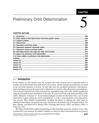
5.3 Lambert’s problem
Suppose we know the position vectors r1 and r2 of two points P1 and P2 on the path of mass m around
mass M, as illustrated in Figure 5.3. r1 and r2 determine the change in the true anomaly Dq, since
cos Dq ¼
r1$r2
r1r2
(5.23)
where
r1 ¼
ffiffiffiffiffiffiffiffiffiffiffi
r1$r1
p
r2 ¼
r2$r2
p
(5.24)
However, if cos Dq 0, then Dq lies in either the first or fourth quadrant, whereas if cos Dq 0, then
Dq lies in the second or third quadrant (recall Figure 3.4). The first step in resolving this quadrant
ambiguity is to calculate the Z component of r1 r2,
ðr1 r2ÞZ ¼ ^
K$ðr1 r2Þ ¼ ^
K$

r1r2 sin Dq^
h

¼ r1r2 sin Dq

^
K$^
w

where ^
w is the unit normal to the orbital plane. Therefore, ^
K$^
w ¼ cos i, where i is the inclination of the
orbit, so that
ðr1 r2ÞZ ¼ r1r2 sin Dq cos i (5.25)
X
Y
Z
r1
r2
r3
Ascending
node
Perigee
50
FIGURE 5.2
Sketch of the orbit of Example 5.1.
5.3 Lambert’s problem 247

We use the sign of the scalar (r1 r2)Z to determine the correct quadrant for Dq.
There are two cases to consider: prograde trajectories (0 i 90) and retrograde trajectories
(90 i 180).
For prograde trajectories (like the one illustrated in Figure 5.3), cos i 0, so that if
(r1 r2)Z 0, then Eqn (5.25) implies that sin Dq 0, which means 0 Dq 180. Since Dq
therefore lies in the first or second quadrant, it follows that Dq is given by cos1ðr1$r2=r1r2Þ. On the
other hand, if (r1 r2)Z 0, Eqn (5.25) implies that sin Dq 0, which means 180 Dq 360. In
this case, Dq lies in the third or fourth quadrant and is given by 360 cos1ðr1$r2=r1r2Þ. For
retrograde trajectories, cos i 0. Thus, if (r1 r2)Z 0 then sin Dq 0, which places Dq in the
third or fourth quadrant. Similarly, if (r1 r2)Z 0, Dq must lie in the first or second quadrant.
This logic can be expressed more concisely as follows:
Dq ¼
cos1

r1$r2
r1r2

if ðr1 r2ÞZ 0
360 cos1

r1$r2
r1r2

if ðr1 r2ÞZ 0
prograde trajectory
cos1

r1$r2
r1r2

if ðr1 r2ÞZ 0
360 cos1

r1$r2
r1r2

if ðr1 r2ÞZ 0
retrograde trajectory
8

:
(5.26)
Y
X
Z
Trajectory
Ascending node
Î
ˆ
K
r1
1
2
Fundamental
plane
ˆ
J
r2
i
i
M
P
P
m
c
ˆ
h
FIGURE 5.3
Lambert’s problem.

J. H. Lambert (1728–1777) was a French-born German astronomer, physicist, and mathemati-
cian. Lambert proposed that the transfer time Dt from P1 to P2 in Figure 5.3 is independent of the
orbit’s eccentricity and depends only on the sum r1 þ r2 of the magnitudes of the position vectors, the
semimajor axis a and the length c of the chord joining P1 and P2. It is noteworthy that the period (of
an ellipse) and the specific mechanical energy are also independent of the eccentricity (Eqns (2.83),
(2.80), and (2.110)).
If we know the time of flight Dt from P1 to P2, then Lambert’s problem is to find the trajectory
joining P1 and P2. The trajectory is determined once we find v1, because, according to Eqns (2.135)
and (2.136), the position and velocity of any point on the path are determined by r1 and v1. That is, in
terms of the notation in Figure 5.3,
r2 ¼ fr1 þ gv1 (5.27a)
v2 ¼ _
fr1 þ _
gv1 (5.27b)
Solving the first of these for v1 yields
v1 ¼
1
g
ðr2 fr1Þ (5.28)
Substitute this result into Eqn (5.27b) to get
v2 ¼ _
fr1 þ
_
g
g
ðr2 fr1Þ ¼
_
g
g
r2
f _
g _
fg
g
r1
However, according to Eqn (2.139), f _
g _
fg ¼ 1. Hence,
v2 ¼
1
g
ð _
gr2 r1Þ (5.29)
By means of Algorithm 4.2, we can find the orbital elements from either r1 and v1 or r2 and v2.
Clearly, Lambert’s problem is solved once we determine the Lagrange coefficients f, g, and _
g.
The Lagrange f and g coefficients and their time derivatives are listed as functions of the change in
true anomaly Dq in Eqns (2.158),
f ¼ 1
mr2
h2
ð1 cosDqÞ g ¼
r1r2
h
sinDq (5.30a)
_
f ¼
m
h
1 cos Dq
sin Dq

m
h2
ð1 cos DqÞ
1
r0

1
r

_
g ¼ 1
mr1
h2
ð1 cos DqÞ (5.30b)
Equations (3.69) expresses these quantities in terms of the universal anomaly c,
f ¼ 1
c2
r1
CðzÞ g ¼ Dt
1
ffiffiffi
m
p c3
SðzÞ (5.31a)
_
f ¼
ffiffiffi
m
p
r1r2
c½zSðzÞ 1 _
g ¼ 1
c2
r2
CðzÞ (5.31b)
where z ¼ ac2
. The f and g functions do not depend on the eccentricity, which would seem to make
them an obvious choice for the solution of Lambert’s problem.

The unknowns on the right of the above sets of equations are h, c, and z, whereas Dq, Dt, r1, and r2
are given. Equating the four pairs of expressions for f, g, _
f, and _
g in Eqns (5.30) and (5.31) yields four
equations in the three unknowns h, c, and z. However, because of the fact that f _
g _
fg ¼ 1, only three
of these equations are independent. We must solve them for h, c, and z in order to evaluate the
Lagrange coefficients and thereby obtain the solution to Lambert’s problem. We will follow the
procedure presented by Bate, Mueller, and White (1971) and Bond and Allman (1996).
While Dq appears throughout Eqn (5.30), the time interval Dt does not. However, Dt does appear in
Eqn (5.31a). A relationship between Dq and Dt can therefore be found by equating the two expressions
for g,
r1r2
h
sin Dq ¼ Dt
1
ffiffiffi
m
p c3
SðzÞ (5.32)
To eliminate the unknown angular momentum h, equate the expressions for f in Eqns (5.30a) and
(5.31a),
1
mr2
h2
ð1 cos DqÞ ¼ 1
c2
r1
CðzÞ
Upon solving this for h, we obtain
h ¼
ffiffiffiffiffiffiffiffiffiffiffiffiffiffiffiffiffiffiffiffiffiffiffiffiffiffiffiffiffiffiffiffiffiffiffiffi
mr1r2ð1 cos DqÞ
c2CðzÞ
s
(5.33)
(Equating the two expressions for _
g leads to the same result.) Substituting Eqn (5.33) into Eqn (5.32),
simplifying, and rearranging the terms yields
ffiffiffi
m
p
Dt ¼ c3
SðzÞ þ c
ffiffiffiffiffiffiffiffiffi
CðzÞ
p

sin Dq
ffiffiffiffiffiffiffiffiffiffiffiffiffiffiffiffiffiffiffiffiffiffi
r1r2
1 cos Dq
r
(5.34)
The term in parentheses on the right is a constant that comprises solely the given data. Let us assign it
the symbol A,
A ¼ sin Dq
r1r2
1 cos Dq
r
(5.35)
Then, Eqn (5.34) assumes the simpler form
ffiffiffi
m
p
Dt ¼ c3
SðzÞ þ Ac
CðzÞ
p
(5.36)
The right side of this equation contains both of the unknown variables c and z. We cannot use the fact
that z ¼ ac2
to reduce the unknowns to one since a is the reciprocal of the semimajor axis of the
unknown orbit.
In order to find a relationship between z and c that does not involve orbital parameters, we equate
the expressions for _
f (Eqns (5.30b) and (5.31b)) to obtain
m
h
1 cos Dq
sin Dq

m
h2
ð1 cos DqÞ
1
r1

1
r2

¼
ffiffiffi
m
p
r1r2
c½zSðzÞ 1

Multiplying through by r1r2 and substituting for the angular momentum using Eqn (5.33) yields
m
ffiffiffiffiffiffiffiffiffiffiffiffiffiffiffiffiffiffiffiffiffiffiffiffiffiffiffiffiffiffiffiffiffiffiffiffi
mr1r2ð1 cos DqÞ
c2CðzÞ
s
1 cos Dq
sin Dq
2
6
6
4
m
mr1r2ð1 cos DqÞ
c2CðzÞ
ð1 cos DqÞ r1 r2
3
7
7
5 ¼
ffiffiffi
m
p
c½zSðzÞ 1
Simplifying and dividing out the common factors leads to
1 cos Dq
p
r1r2
p
sin Dq
CðzÞ
p
c2
CðzÞ r1 r2 ¼ zSðzÞ 1
We recognize the reciprocal of A on the left, so we can rearrange this expression to read as follows:
c2
CðzÞ ¼ r1 þ r2 þ A
zSðzÞ 1
CðzÞ
p
The right-hand side depends exclusively on z. Let us call that function y(z), so that
c ¼
yðzÞ
CðzÞ
s
(5.37)
where
yðzÞ ¼ r1 þ r2 þ A
zSðzÞ 1
CðzÞ
p (5.38)
Equation (5.37) is the relation between c and z that we were seeking. Substituting it back into Eqn
(5.36) yields
ffiffiffi
m
p
Dt ¼

yðzÞ
CðzÞ
3
2
SðzÞ þ A
yðzÞ
p
(5.39)
We can use this equation to solve for z, given the time interval Dt. It must be done iteratively.
Using Newton’s method, we form the function
FðzÞ ¼

yðzÞ
CðzÞ
3
2
SðzÞ þ A
yðzÞ
p

ffiffiffi
m
p
Dt (5.40)
and its derivative
F0
ðzÞ ¼
1
2
ffiffiffiffiffiffiffiffiffiffiffiffiffiffiffiffiffiffiffi
yðzÞC5ðzÞ
p
n
½2CðzÞS0
ðzÞ 3C0
ðzÞSðzÞy2
ðzÞ þ
h
AC
5
2ðzÞ þ 3CðzÞSðzÞyðzÞ
i
y0
ðzÞ
o
(5.41)
in which C0ðzÞ and S0ðzÞ are the derivatives of the Stumpff functions, which are given by Eqn (3.63).
y0ðzÞ is obtained by differentiating y (z) in Eqn (5.38),
y0
ðzÞ ¼
A
2CðzÞ
3
2

½1 zSðzÞC0
ðzÞ þ 2½SðzÞ þ zS0
ðzÞCðzÞ


If we substitute Eqn (3.63) into this expression, a much simpler form is obtained, namely
y0
ðzÞ ¼
A
4
ffiffiffiffi
C
p
(5.42)
This result can be worked out by using Eqns (3.52) and (3.53) to express C(z) and S(z) in terms of the
more familiar trig functions. Substituting Eqn (5.42) along with Eqn (3.63) into Eqn (5.41) yields
F0
ðzÞ ¼
8

:

yðzÞ
CðzÞ
3
2
(
1
2z

CðzÞ
3
2
SðzÞ
CðzÞ

þ
3
4
SðzÞ2
CðzÞ
)
þ
A
8

3
SðzÞ
CðzÞ
yðzÞ
p
þ A
CðzÞ
yðzÞ
s #
ðzs0Þ
ffiffiffi
2
p
40
yð0Þ
3
2 þ
A
8

yð0Þ
p
þ A
1
2yð0Þ
s #
ðz ¼ 0Þ
(5.43)
Evaluating F0ðzÞ at z ¼ 0 must be done carefully (and is therefore shown as a special case) because
of the z in the denominator within the curly brackets. To handle z ¼ 0, we assume that z is very small
(almost but not quite zero) so that we can retain just the first two terms in the series expansions of C(z)
and S(z) (Eqn (3.51)),
CðzÞ ¼
1
2

z
24
þ / SðzÞ ¼
1
6

z
120
þ /
Then, we evaluate the term within the curly brackets as follows:
1
2z

CðzÞ
3
2
SðzÞ
CðzÞ

z
1
2z
2
6
4

1
2

z
24

3
2

1
6

z
120

1
2

z
24

3
7
5
¼
1
2z

1
2

z
24

3

1
6

z
120

1
z
12
1
#
z
1
2z

1
2

z
24

3

1
6

z
120

1 þ
z
12
#
¼
1
2z

7z
120
þ
z2
480

¼
7
240
þ
z
960
In the third step, we used the familiar binomial expansion theorem,
ða þ bÞn
¼ an
þ nan1
b þ
nðn 1Þ
2!
an2
b2
þ
nðn 1Þðn 2Þ
3!
an3
b3
þ / (5.44)
to set (1z/12)1
z 1 þ z/12, which is true if z is close to zero. Thus, when z is actually zero,
1
2z

CðzÞ
3
2
SðzÞ
CðzÞ

¼
7
240

Evaluating the other terms in F0ðzÞ presents no difficulties.
F(z) in Eqn (5.40) and F0ðzÞ in Eqn (5.43) are used in Newton’s formula, Eqn (3.16), for the
iterative procedure,
ziþ1 ¼ zi
FðziÞ
F0ðziÞ
(5.45)
For choice of a starting value for z, recall that z ¼ (1/a)c2
. According to Eqn (3.57), z ¼ E2
for an
ellipse and z ¼ F2
for a hyperbola. Since we do not know what the orbit is, setting z0 ¼ 0 seems a
reasonable, simple choice. Alternatively, one can plot or tabulate F(z) and choose z0 to be a point near
where F(z) changes sign.
Substituting Eqns (5.37) and (5.39) into Eqn (5.31) yields the Lagrange coefficients as functions of
z alone.
f ¼ 1
2
4
yðzÞ
CðzÞ
s 3
5
2
r1
CðzÞ ¼ 1
yðzÞ
r1
(5.46a)
g ¼
1
ffiffiffi
m
p

yðzÞ
CðzÞ
3
2
SðzÞ þ A
yðzÞ
p

1
ffiffiffi
m
p

yðzÞ
CðzÞ
3
2
SðzÞ ¼ A
yðzÞ
m
s
(5.46b)
_
f ¼
ffiffiffi
m
p
r1r2
yðzÞ
CðzÞ
s
½zSðzÞ 1 (5.46c)
_
g ¼ 1
2
4
yðzÞ
CðzÞ
s 3
5
2
r2
CðzÞ ¼ 1
yðzÞ
r2
(5.46d)
We are now in a position to present the solution of Lambert’s problem in universal variables, following
Bond and Allman (1996).
n
ALGORITHM 5.2
Solve Lambert’s problem. A MATLAB implementation appears in Appendix D.25.
Given r1, r2, and Dt, the steps are as follows:
1. Calculate r1 and r2 using Eqn (5.24).
2. Choose either a prograde or a retrograde trajectory and calculate Dq using Eqn (5.26).
3. Calculate A in Eqn (5.35).
4. By iteration, using Eqns (5.40), (5.43), and (5.45), solve Eqn (5.39) for z. The sign of z tells us
whether the orbit is a hyperbola (z 0), parabola (z ¼ 0), or ellipse (z 0).
5. Calculate y using Eqn (5.38).
6. Calculate the Lagrange f, g, and _
g functions using Eqn (5.46).
7. Calculate v1 and v2 from Eqns (5.28) and (5.29).
8. Use r1 and v1 (or r2 and v2) in Algorithm 4.2 to obtain the orbital elements.
n

EXAMPLE 5.2
The position of an earth satellite is first determined to be r1 ¼ 5000^
I þ 10,000^
J þ 2100^
K ðkmÞ. After one hour the
position vector is r2 ¼ 14,600^
I þ 2500^
J þ 7000^
K ðkmÞ. Determine the orbital elements and find the perigee
altitude and the time since perigee passage of the first sighting.
Solution
We first must execute the steps of Algorithm 5.2 in order to find v1 and v2.
Step 1:
r1 ¼
ffiffiffiffiffiffiffiffiffiffiffiffiffiffiffiffiffiffiffiffiffiffiffiffiffiffiffiffiffiffiffiffiffiffiffiffiffiffiffiffiffiffiffiffiffiffiffiffiffiffiffiffiffiffiffiffiffiffiffi
ffi
50002 þ 10,0002 þ 21002
p
¼ 11,375 km
r2 ¼
ffiffiffiffiffiffiffiffiffiffiffiffiffiffiffiffiffiffiffiffiffiffiffiffiffiffiffiffiffiffiffiffiffiffiffiffiffiffiffiffiffiffiffiffiffiffiffiffiffiffiffiffiffiffiffiffiffiffiffiffiffiffiffiffiffiffiffi
ð14,600Þ2
þ 25002 þ 70002
q
¼ 16,383 km
Step 2: Assume a prograde trajectory.
r1 r2 ¼

64:75^
I 65:66^
J þ 158:5^
K

106
cos1r1$r2
r1r2
¼ 100:29
Since the trajectory is prograde and the z component of r1 r2 is positive, it follows from Eqn (5.26) that
Dq ¼ 100:29
Step 3:
A ¼ sin Dq
ffiffiffiffiffiffiffiffiffiffiffiffiffiffiffiffiffiffiffiffiffiffiffi
r1r2
1 cos Dq
r
¼ sin 100:29
ffiffiffiffiffiffiffiffiffiffiffiffiffiffiffiffiffiffiffiffiffiffiffiffiffiffiffiffiffiffiffiffiffiffiffiffiffiffiffi
11,375 16,383
1 cos 100:29
r
¼ 12,372 km
Step 4:
Using this value of A and Dt ¼ 3600 s, we can evaluate the functions F(z) and F0ðzÞ given by Eqns (5.40)
and (5.43), respectively. Let us first plot F(z) to estimate where it crosses the z-axis. As can be seen from
Figure 5.4, F(z) ¼ 0 near z ¼ 1.5. With z0 ¼ 1.5 as our initial estimate, we execute Newton’s procedure
(Eqn (5.45)):
ziþ1 ¼ zi
FðziÞ
F0ðziÞ
1 2
0
F(z)
z
5 105
×
− ×
5 105
FIGURE 5.4
Graph of F(z).

z1 ¼ 1:5
14,476:4
362,642
¼ 1:53991
z2 ¼ 1:53991
23:6274
363,828
¼ 1:53985
z3 ¼ 1:53985
6:29457 105
363,826
¼ 1:53985
Thus, to five significant figures z ¼ 1.5398. The fact that z is positive means the orbit is an ellipse.
Step 5:
y ¼ r1 þ r2 þ A
zSðzÞ 1
ffiffiffiffiffiffiffiffiffiffi
CðzÞ
p ¼ 11,375 þ 16,383 þ 12,372
1:5398Sð1:5398Þ
ffiffiffiffiffiffiffiffiffiffiffiffiffiffiffiffiffiffiffiffiffiffiffiffi
Cð1:5398Þ
p ¼ 13,523 km
Step 6:
Equation (5.46) yields the Lagrange functions
f ¼ 1
y
r1
¼ 1
13,523
11,375
¼ 0:18877
g ¼ A
ffiffiffi
y
m
r
¼ 12,372
ffiffiffiffiffiffiffiffiffiffiffiffiffiffiffiffiffiffiffiffi
13,523
398,600
r
¼ 2278:9 s
_
g ¼ 1
y
r2
¼ 1
13,523
16,383
¼ 0:17457
Step 7:
v1 ¼
1
g
ðr2 fr1Þ ¼
1
2278:9
h
14,600^
I þ 2500^
J þ 7000^
K

ð0:18877Þ

5000^
I þ 10,000^
J þ 2100^
K
i
v1 ¼ 5:9925^
I þ 1:9254^
J þ 3:2456^
K ðkmÞ
v2 ¼
1
g
ð _
gr2 r1Þ ¼
1
2278:9
h
ð0:17457Þ

14,600^
I þ 2500^
J þ 7000^
K

5000^
I þ 10,000^
J þ 2100^
K
i
v2 ¼ 3:3125^
I 4:1966^
J 0:38529^
K ðkmÞ
Step 8:
Using r1 and v1 Algorithm 4.2 yields the orbital elements:
h ¼ 80,470 km2
=s
a ¼ 20,000 km
e ¼ 0:4335
U ¼ 44:60
i ¼ 30:19
u ¼ 30:71
q1 ¼ 350:8

This elliptical orbit is plotted in Figure 5.5. The perigee of the orbit is
rp ¼
h2
m
1
1 þ e cos ð0Þ
¼
80,4702
398,600
1
1 þ 0:4335
¼ 11,330 k
Therefore, the perigee altitude is 11330 6378 ¼ 4952 km .
To find the time of the first sighting, we first calculate the eccentric anomaly by means of Eqn (3.13b),
E1 ¼ 2tan1
ffiffiffiffiffiffiffiffiffiffiffiffi
1 e
1 þ e
r
tan
q
2
!
¼ 2 tan 1
ffiffiffiffiffiffiffiffiffiffiffiffiffiffiffiffiffiffiffiffiffiffiffiffiffi
1 0:4335
1 þ 0:4335
r
tan
350:8
2
!
¼ 2tan1
ð0:05041Þ
¼ 0:1007 rad
Then using Kepler’s equation for the ellipse (Eqn (3.14)), the mean anomaly is found to be
Me1
¼ E1 e sin E1 ¼ 0:1007 0:4335 sin ð0:1007Þ ¼ 0:05715 rad
so that from Eqn (3.7), the time since perigee passage is
t1 ¼
h3
m2
1
1 e2
3
2
Me1
¼
80,4703
398,6002
1
1 :43352
3
2
ð0:05715Þ ¼ 256:1 s
The minus sign means that there are 256.1 s until perigee encounter after the initial sighting.
FIGURE 5.5
The solution of Example 5.2 (Lambert’s problem).

EXAMPLE 5.3
A meteoroid is sighted at an altitude of 267,000 km. After 13.5 hours and a change in true anomaly of 5, the
altitude is observed to be 140,000 km. Calculate the perigee altitude and the time to perigee after the second
sighting.
Solution
We have
P1 : r1 ¼ 6378 þ 267,000 ¼ 273,378 km
P2 : r2 ¼ 6378 þ 140,000 ¼ 146,378 km
Dt ¼ 13:5 3600 ¼ 48,600 s
Dq ¼ 5
Since r1, r2, and Dq are given, we can skip to Step 3 of Algorithm 5.2 and compute
A ¼ 2:8263 105
km
Then, solving for z as in the previous example, we obtain
z ¼ 0:17344
Since z is negative, the path of the meteoroid is a hyperbola.
With z available, we evaluate the Lagrange functions,
f ¼ 0:95846
g ¼ 47,708 s
_
g ¼ 0:92241
(a)
Step 7 requires the initial and final position vectors. Therefore, for purposes of this problem, let us define a
geocentric coordinate system with the x-axis aligned with r1 and the y-axis at 90 thereto in the direction of the
motion (Figure 5.6). The z-axis is therefore normal to the plane of the orbit. Then,
r1 ¼ r1
^
i ¼ 273; 378^
i ðkmÞ
r2 ¼ r2 cos Dq^
i þ r2 sin Dq^
j ¼ 145,820^
i þ 12,758^
j ðkmÞ
(b)
P1
P2
210.16
205.16
273,378 km
146,378 km
r1
r2
x
y
FIGURE 5.6
Solution of Example 5.3 (Lambert’s problem).

With Eqns (a) and (b), we obtain the velocity at P1,
v1 ¼
1
g
ðr2 fr1Þ
¼
1
47,708
h
145,820^
i þ 12,758^
j

0:95846

273,378^
i
i
¼ 2:4356^
i þ 0:26741^
j ðkm=sÞ
Using r1 and v1, Algorithm 4.2 yields
h ¼ 73,105 km2
=s
e ¼ 1:0506
q1 ¼ 205:16
The orbit is now determined except for its orientation in space, for which no information was provided. In the
plane of the orbit, the trajectory is as shown in Figure 5.6.
The perigee radius is
rp ¼
h2
m
1
1 þ e cos ð0Þ
¼ 6538:2 km
which means the perigee altitude is dangerously low for a large meteoroid,
zp ¼ 6538:2 6378 ¼ 160:2 kmð100 milesÞ
To find the time of flight from P2 to perigee, we note that the true anomaly of P2 is
q2 ¼ q1 þ 5
¼ 210:16
The hyperbolic eccentric anomaly F2 follows from Eqn (3.44a),
F2 ¼ 2 tan h1
ffiffiffiffiffiffiffiffiffiffiffiffi
e 1
e þ 1
r
tan
q2
2
!
¼ 1:3347 rad
Substituting this value into Kepler’s equation (Eqn (3.40)) yields the mean anomaly Mh,
Mh2
¼ e sin hðF2Þ F2 ¼ 0:52265 rad
Finally, Eqn (3.34) yields the time
t2 ¼
Mh2
h3
m2 e2 1
3
2
¼ 38,396 s
The minus sign means that 38,396 s (a scant 10.6 h) remain until the meteoroid passes through perigee.
5.4 Sidereal time
To deduce the orbit of a satellite or celestial body from observations requires, among other things,
recording the time of each observation. The time we use in everyday life, the time we set our clocks by,
is the solar time. It is reckoned by the motion of the sun across the sky. A solar day is the time required
for the sun to return to the same position overhead, that is, to lie on the same meridian. A solar

daydfrom high noon to high noondcomprises 24 h. Universal time (UT) is determined by the sun’s
passage across the Greenwich meridian, which is zero degrees terrestrial longitude. See Figure 1.18. At
noon UT, the sun lies on the Greenwich meridian. Local standard time, or civil time, is obtained from
the UT by adding 1 h for each time zone between Greenwich and the site, measured westward.
Sidereal time is measured by the rotation of the earth relative to the fixed stars (i.e., the celestial
sphere, Figure 4.3). The time it takes for a distant star to return to its same position overhead, that is, to
lie on the same meridian, is one sidereal day (24 sidereal hours). As illustrated in Figure 4.20, the
earth’s orbit around the sun results in the sidereal day being slightly shorter than the solar day. One
sidereal day is 23 hours and 56 minutes. To put it another way, the earth rotates 360 in one sidereal
day, whereas it rotates 360.986 in a solar day.
Local sidereal time q of a site is the time elapsed since the local meridian of the site passed through
the vernal equinox. The number of degrees (measured eastward) between the vernal equinox and the
local meridian is the sidereal time multiplied by 15. To know the location of a point on the earth at any
given instant relative to the geocentric equatorial frame requires knowing its local sidereal time. The
local sidereal time of a site is found by first determining the Greenwich sidereal time qG (the sidereal
time of the Greenwich meridian) and then adding the east longitude (or subtracting the west longitude)
of the site. Algorithms for determining sidereal time rely on the notion of Julian day.
The Julian day number is the number of days since noon UT on January 1, 4713 BC. The origin of
this time scale is placed in antiquity so that, except for prehistoric events, we do not have to deal with
positive and negative dates. The Julian day count is uniform and continuous and does not involve leap
years or different numbers of days in different months. The number of days between two events is
found by simply subtracting the Julian day of one from that of the other. The JD begins at noon rather
than at midnight so that astronomers observing the heavens at night would not have to deal with a
change of date during their watch.
The Julian day numbering system is not to be confused with the Julian calendar, which the Roman
emperor Julius Caesar introduced in 46 BC. The Gregorian calendar, introduced in 1583, has largely
supplanted the Julian calendar and is in common civil use today throughout much of the world.
J0 is the symbol for the Julian day number at 0 h UT (which is halfway into the Julian day). At any
other UT, the Julian day is given by
JD ¼ J0 þ
UT
24
(5.47)
Algorithms and tables for obtaining J0 from the ordinary year (y), month (m), and day (d) exist in
the literature and on the World Wide Web. One of the simplest formulas is found in Boulet (1991),
J0 ¼ 367y INT
8

:
7
h
y þ INT

mþ9
12
i
4
9

=

;
þ INT

275m
9

þ d þ 1,721,013:5 (5.48)
where y, m, and d are integers lying in the following ranges:
1901 y 2099
1 m 12
1 d 31
5.4 Sidereal time 259

INT (x) means to retain only the integer portion of x, without rounding (or, in other words, round
toward zero), that is, INT (3.9) ¼ 3 and INT (3.9) ¼ 3. Appendix D.26 lists a MATLAB imple-
mentation of Eqn (5.48).
EXAMPLE 5.4
What is the Julian day number for May 12, 2004, at 14:45:30 UT?
Solution
In this case y ¼ 2004, m ¼ 5, and d ¼ 12. Therefore, Eqn (5.48) yields the Julian day number at 0 h UT,
J0 ¼ 367 2004 INT
8

:
7

2004 þ

5 þ 9
12

4
9

=

;
þ INT

275 5
9

þ 12 þ 1,721,013:5
¼ 735,468 INT

7½2004 þ 1
4

þ 152 þ 12 þ 1,721,013:5
¼ 735,468 3508 þ 152 þ 12 þ 1,721,013:5
or
J0 ¼ 2,453,137:5 days
The universal time, in hours, is
UT ¼ 14 þ
45
60
þ
30
3600
¼ 14:758 h
Therefore, from Eqn (5.47), we obtain the Julian day number at the desired universal time,
JD ¼ 2,453,137:5 þ
14:758
24
¼ 2,453,138:115 days
EXAMPLE 5.5
Find the elapsed time between October 4, 1957 UT 19:26:24, and the date of the previous example.
Solution
Proceeding as in Example 5.4 we find that the Julian day number of the given event (the launch of the first man-
made satellite, Sputnik I) is
JD1 ¼ 2,436,116:3100 days
The JD of the previous example is
JD2 ¼ 2,453,138:1149 days
Hence, the elapsed time is
DJD ¼ 2,453,138:1149 2,436,116:3100 ¼ 17,021:805 days ð46 years; 220 daysÞ

The current Julian epoch is defined to have been noon on January 1, 2000. This epoch is denoted
J2000 and has the exact Julian day number 2,451,545.0. Since there are 365.25 days in a Julian year, a
Julian century has 36,525 days. It follows that the time T0 in Julian centuries between the Julian day J0
and J2000 is
T0 ¼
J0 2,451,545
36,525
(5.49)
The Greenwich sidereal time qG0 at 0 h UT may be found in terms of this dimensionless time
(Seidelmann, 1992; Section 2.24). qG0 is in degrees and is given by the series
qG0 ¼ 100:4606184 þ 36,000:77004T0 þ 0:000387933T2
0 2:583 108
T3
0 ðdegreesÞ (5.50)
This formula can yield a value outside the range 0 qG0 360. If so, then the appropriate integer
multiple of 360 must be added or subtracted to bring qG0 into that range.
Once qG0 has been determined, the Greenwich sidereal time qG at any other UT is found using the
relation
qG ¼ qG0 þ 360:98564724
UT
24
(5.51)
where UT is in hours. The coefficient of the second term on the right is the number of degrees the earth
rotates in 24 h (solar time).
Finally, the local sidereal time q of a site is obtained by adding its east longitude L to the
Greenwich sidereal time,
q ¼ qG þ L (5.52)
Here again, it is possible for the computed value of q to exceed 360. If so, it must be reduced to within
that limit by subtracting the appropriate integer multiple of 360. Figure 5.7 illustrates the relationship
among qG0, qG, L, and q.
North
pole
Site
Greenwich
G0
G
Greenwich
at 0 h UT
FIGURE 5.7
Schematic of the relationship among qG0, qG, L, and q.
5.4 Sidereal time 261

n
ALGORITHM 5.3
Calculate the local sidereal time, given the date, the local time, and the east longitude of the site.
This is implemented in MATLAB in Appendix D.27.
1. Using the year, month, and day, calculate J0 using Eqn (5.48).
2. Calculate T0 by means of Eqn (5.49).
3. Compute qG0 from Eqn (5.50). If qG0 lies outside the range 0
qG0 360
, then subtract the
multiple of 360
required to place qG0 in that range.
4. Calculate qG using Eqn (5.51).
5. Calculate the local sidereal time q by means of Eqn (5.52), adjusting the final value so it lies
between 0
and 360
.
n
EXAMPLE 5.6
Use Algorithm 5.3 to find the local sidereal time (in degrees) of Tokyo, Japan, on March 3, 2004, at 4:30:00 UT.
The east longitude of Tokyo is 139.80. (This places Tokyo nine time zones ahead of Greenwich, so the local time
is 1:30 in the afternoon.)
Step 1:
J0 ¼ 367 2004 INT
8

:
7

2004 þ INT 3þ9
12

4
9

=

;
þ INT

275 3
9

þ 3 þ 1,721,013:5
¼ 2,453,067:5 days
Recall that the 0.5 means that we are halfway into the Julian day, which began at noon UT of the previous day.
Step 2:
T0 ¼
2,453,067:5 2,451,545
36,525
¼ 0:041683778
Step 3:
qG0 ¼ 100:4606184 þ 36,000:77004ð0:041683778Þ
þ 0:000387933ð0:041683778Þ2
2:583 108 ð0:041683778Þ3
¼ 1601:1087
The right-hand side is too large. We must reduce qG0 to an angle that does not exceed 360. To that end,
observe that
INTð1601:1087=360Þ ¼ 4
Hence,
qG0 ¼ 1601:1087 4 360 ¼ 161:10873
(a)

Step 4:
The UT of interest in this problem is
UT ¼ 4 þ
30
60
þ
0
3600
¼ 4:5 h
Substitute this and Eqn (a) into Eqn (5.51) to get the Greenwich sidereal time.
qG ¼ 161:10873 þ 360:98564724
4:5
24
¼ 228:79354
Step 5:
Add the east longitude of Tokyo to this value to obtain the local sidereal time,
q ¼ 228:79354 þ 139:80 ¼ 368:59
To reduce this result into the range 0 q 360, we must subtract 360 to get
q ¼ 368:59 360 ¼ 8:59ð0:573 hÞ
Observe that the right ascension of a celestial body lying on Tokyo’s meridian is 8.59.
5.5 Topocentric coordinate system
A topocentric coordinate system is one that is centered at the observer’s location on the surface of the
earth. Consider an object Bda satellite or celestial bodydand an observer O on the earth’s surface, as
illustrated in Figure 5.8. r is the position of the body B relative to the center of attraction C; R is the
position vector of the observer relative to C; and r is the position of the body B relative to the observer.
r, R, and r comprise the fundamental vector triangle. The relationship among these three vectors is
r ¼ R þ r (5.53)
As we know, the earth is not a sphere but a slightly oblate spheroid. This ellipsoidal shape is
exaggerated in Figure 5.8. The location of the observation site O is determined by specifying its east
longitude L and latitude f. East longitude L is measured positive eastward from the Greenwich
meridian to the meridian through O. The angle between the vernal equinox direction (XZ plane) and the
meridian of O is the local sidereal time q. Likewise, qG is the Greenwich sidereal time. Once we know
qG, then the local sidereal time is given by Eqn (5.52).
Latitude f is the angle between the equator and the normal ^
n to the earth’s surface at O. Since the
earth is not a perfect sphere, the position vector R, directed from the center C of the earth to O, does not
point in the direction of the normal except at the equator and the poles.
The oblateness, or flattening f, was defined in Section 4.7,
f ¼
Re Rp
Re
where Re is the equatorial radius and Rp is the polar radius. (Review from Table 4.3 that
f ¼ 0.00335 for the earth.) Figure 5.9 shows the ellipse of the meridian through O. Obviously,
5.5 Topocentric coordinate system 263

C
φ
Equator
Re
O
′
φ
North
pole
Rp
Tangent
′
C
Rφe2sinφ
x'
z'
R
R
φ
′
zO
′
xO
FIGURE 5.9
The relationship between geocentric latitude ðf0Þ and geodetic latitude (f).
X
ˆ
I
Ĵ
ˆ
K
Local meridian
Polar axis
Z ,
,z
Y
x
(East longitude)
C
O
Re
R
Rp
C' (latitude)
R
n̂
B (tracked object)
r
G
Greenwich meridian
Equator
γ
θ
θ
Λ
φ
φ
FIGURE 5.8
Oblate spheroidal earth (exaggerated).

Re and Rp are, respectively, the semimajor and semiminor axes of the ellipse. According to
Eqn (2.76),
Rp ¼ Re
ffiffiffiffiffiffiffiffiffiffiffiffiffi
1 e2
p
It is easy to show from the above two relations that flattening and eccentricity are related as
follows:
e ¼
ffiffiffiffiffiffiffiffiffiffiffiffiffiffiffi
2f f2
p
f ¼ 1
ffiffiffiffiffiffiffiffiffiffiffiffiffi
1 e2
p
As illustrated in Figure 5.8 and again in Figure 5.9, the normal to the earth’s surface at O intersects
the polar axis at a point C0 that lies below the center C of the earth (if O is in the northern hemisphere).
The angle f between the normal and the equator is called the geodetic latitude, as opposed to
geocentric latitude f0, which is the angle between the equatorial plane and the line joining O to the
center of the earth. The distance from C to C0 is Rf e2
sin2
f, where Rf, the distance from C0 to O, is a
function of latitude (Seidelmann, 1992; Section 4.22)
Rf ¼
Re
ffiffiffiffiffiffiffiffiffiffiffiffiffiffiffiffiffiffiffiffiffiffiffi
1 e2sin2
f
p ¼
Re
ffiffiffiffiffiffiffiffiffiffiffiffiffiffiffiffiffiffiffiffiffiffiffiffiffiffiffiffiffiffiffiffiffiffiffiffiffi
1 ð2f f2Þsin2
f
q (5.54)
Thus, the meridional coordinates of O are
x0
O ¼ Rf cos f
z0
O ¼ 1 e2 Rf sin f ¼ ð1 fÞ2
Rf sin f
If the observation point O is at an elevation H above the ellipsoidal surface, then we must add H cos
f to x0
O and H sin f to z0
O to obtain
x0
O ¼ Rc cos f z0
O ¼ Rs sin f (5.55a)
where
Rc ¼ Rf þ H Rs ¼ ð1 fÞ2
Rf þ H (5.55b)
Observe that whereas Rc is the distance of O from point C0 on the earth’s axis, Rs is the distance from O
to the intersection of the line OC0 with the equatorial plane.
The geocentric equatorial coordinates of O are
X ¼ x0
O cos q Y ¼ x0
O sin q Z ¼ z0
O
where q is the local sidereal time given in Eqn (5.52). Hence, the position vector R shown in
Figure 5.8 is
R ¼ Rc cos f cos q^
I þ Rc cos f sin q^
J þ Rs sin f^
K
Substituting Eqns (5.54) and (5.55b) yields
R ¼

Re
1 ð2f f 2Þsin2
f
q þ H
#
cos f

cos q^
I þ sin q^
J

þ

Reð1 fÞ2
1 ð2f f2Þsin2
f
q þ H
#
sin f^
K
(5.56)
5.5 Topocentric coordinate system 265

In terms of the geocentric latitude f0,
R ¼ Re cos f0
cos q^
I þ Re cos f0
sin q^
J þ Re sin f0 ^
K
By equating these two expressions for R and setting H ¼ 0, it is easy to show that at sea level the
geodetic latitude is related to geocentric latitude f0 as follows:
tan f0
¼ ð1 fÞ2
tan f
5.6 Topocentric equatorial coordinate system
The topocentric equatorial coordinate system with the origin at point O on the surface of the earth uses
a nonrotating set of xyz axes through O which coincide with the XYZ axes of the geocentric equatorial
frame, as illustrated in Figure 5.10. As can be inferred from the figure, the relative position vector r in
terms of the topocentric right ascension and declination is
r ¼ r cos d cos a^
I þ r cos d sin a^
J þ r sin d^
K
since at all times, ^
i ¼ ^
I, ^
j ¼ ^
J, and ^
k ¼ ^
K for this frame of reference. We can write r as
r ¼ r^
r
X
g
ˆ
I
ˆ
J
ˆ
K
Y
q
C
O
R
Re
r
ρ
ρ
Z
g
x
y
z
a
d
B
f ’
Equator
ˆ
i
ˆ
j
ˆ
k
FIGURE 5.10
Topocentric equatorial coordinate system.

where r is the slant range and ^
r is the unit vector in the direction of the position vector r,
^
r ¼ cos d cos a^
I þ cos d sin a^
J þ sin d^
K (5.57)
Since the origins of the geocentric and topocentric systems do not coincide, the direction cosines of
the position vectors r and r will in general differ. In particular the topocentric right ascension and
declination of an earth-orbiting body B will not be the same as the geocentric right ascension and
declination. This is an example of parallax. On the other hand, if krk[kRk, then the difference
between the geocentric and topocentric position vectors, and hence, the right ascension and declina-
tion, is negligible. This is true for the distant planets and stars.
EXAMPLE 5.7
At the instant when the Greenwich sidereal time is qG ¼ 126.7, the geocentric equatorial position vector of the
International Space Station is
r ¼ 5368^
I 1784^
J þ 3691^
K ðkmÞ
Find its topocentric right ascension and declination at sea level (H ¼ 0), latitude f ¼ 20, and east longitude
L ¼ 60.
Solution
According to Eqn (5.52), the local sidereal time at the observation site is
q ¼ qG þ L ¼ 126:7 þ 60 ¼ 186:7
Substituting Re ¼ 6378 km, f ¼ 0.003353 (Table 4.3), q ¼ 189.7, and f ¼ 20 into Eqn (5.56) yields the
geocentric position vector of the site,
R ¼ 5955^
I 699:5^
J þ 2168^
K ðkmÞ
Having found R, we obtain the position vector of the space station relative to the site from Eqn (5.53),
r ¼ r R
¼

5368^
I 1784^
J þ 3691^
K

5955^
I 699:5^
J þ 2168^
K

¼ 586:8^
I 1084^
J þ 1523^
K ðkmÞ
Applying Algorithm 4.1 to this vector yields
a ¼ 298:4
d ¼ 51:01
Compare these with the geocentric right ascension a0 and declination d0, which were computed in
Example 4.1,
a0 ¼ 198:4
d0 ¼ 33:12
5.7 Topocentric horizon coordinate system
The topocentric horizon coordinate system was introduced in Section 1.7 and is illustrated again in
Figure 5.11. It is centered at the observation point O whose position vector is R. The xy plane is the
5.7 Topocentric horizon coordinate system 267

local horizon, which is the plane tangent to the ellipsoid at point O. The z-axis is normal to this plane
directed outward toward the zenith. The x-axis is directed eastward and the y-axis points north.
Because the x-axis points east, this may be referred to as an ENZ (East–North–Zenith) frame. In the
SEZ topocentric reference frame the x-axis points toward the south and the y-axis toward the east. The
SEZ frame is obtained from ENZ by a 90 clockwise rotation around the zenith. Therefore, the matrix
of the transformation from NEZ to SEZ is [R3 (90)], where [R3 (f)] is found in Eqn (4.34).
The position vector r of a body B relative to the topocentric horizon system in Figure 5.11 is
r ¼ r cos a sin A^
i þ r cos a cos A^
j þ r sin a^
k
in which r is the range; A is the azimuth measured positive clockwise from due north (0 A 360);
and a is the elevation angle or altitude measured from the horizontal to the line of sight of the body B
(90 a 90). The unit vector ^
r in the line of sight direction is
^
r ¼ cos a sin A^
i þ cos a cos A^
j þ sin a^
k (5.58)
The transformation between geocentric equatorial and topocentric horizon systems is found by first
determining the projections of the topocentric base vectors^
i^
j^
k onto those of the geocentric equatorial
frame. From Figure 5.11, it is apparent that
^
k ¼ cos f^
i
0
þ sin f^
K
X
ˆ
I
ˆ
J
ˆ
K
Y
C
O
R
Z
x (East)
z (Zenith)
î
k̂
B
A
a
ĵ
y
(North)
C
ˆ
î
Equator
γ
θ
φ
FIGURE 5.11
Topocentric horizon (xyz) coordinate system on the surface of the oblate earth.

and
^
i
0
¼ cos q^
I þ sin q^
J
where ^
i
0
lies in the local meridional plane and is normal to the Z-axis. Hence,
^
k ¼ cos f cos q^
I þ cos f sin q^
J þ sin f^
K (5.59)
The eastward-directed unit vector ^
i may be found by taking the cross product of ^
K into the unit
normal ^
k,
^
i ¼
^
K ^
k

^
K ^
k

¼
cos f sin q^
I þ cos f cos q^
J
ffiffiffiffiffiffiffiffiffiffiffiffiffiffiffiffiffiffiffiffiffiffiffiffiffiffiffiffiffiffiffiffiffiffiffiffiffiffiffiffiffiffi
cos2fðsin2
q þ cos2qÞ
q ¼ sin q^
I þ cos q^
J (5.60)
Finally, crossing ^
k into ^
i yields ^
j,
^
j ¼ ^
k ^
i ¼
^
I ^
J ^
K
cos f cos q cos f sin q sin f
sin q cos q 0
¼ sin f cos q^
I sin f sin q^
J þ cos f^
K (5.61)
Let us denote the matrix of the transformation from the geocentric equatorial to the topocentric
horizon as [Q]Xx. Recall from Section 4.5 that the rows of this matrix comprise the direction cosines of
^
i, ^
j, and ^
k, respectively. It follows from Eqns (5.59)–(5.61) that
½QXx ¼
2
4
sin q cos q 0
sin f cos q sin f sin q cos f
3
5 (5.62a)
The reverse transformation, from the topocentric horizon to the geocentric equatorial, is represented by
the transpose of this matrix,
½QxX ¼
2
4
sin q sin f cos q cos f cos q
cos q sin f sin q cos f sin q
0 cos f sin f
3
5 (5.62b)
Observe that these matrices also represent the transformation between the topocentric horizon and the
topocentric equatorial frames, because the unit basis vectors of the latter coincide with those of the
geocentric equatorial coordinate system.
EXAMPLE 5.8
The east longitude and latitude of an observer near San Francisco are L ¼ 238 and f ¼ 38, respectively. The
local sidereal time is q ¼ 215.1 (14 h 20 min). At that time, the planet Jupiter is observed by means of a tele-
scope to be located at azimuth A ¼ 214.3 and angular elevation a ¼ 43. What are Jupiter’s right ascension and
declination in the topocentric equatorial system?
Solution
The given information allows us to formulate the matrix of the transformation from the topocentric horizon to the
topocentric equatorial using Eqn (5.62b),
½QxX ¼
2
4
sin 215:1 sin 38cos 215:1 cos 38cos 215:1
cos 215:1 sin 38sin 215:1 cos 38sin 215:1
0 cos 38 sin 38
3
5 ¼
2
4
0:5750 0:5037 0:6447
0:8182 0:3540 0:4531
0 0:7880 0:6157
3
5

From Eqn (5.58), we have
^
r ¼ cos a sin A^
i þ cos a cos A^
j þ sin a^
k
¼ cos 43
sin 214:3^
i þ cos 43
cos 214:3^
j þ sin 43^
k
¼ 0:4121^
i 0:6042^
j þ 0:6820^
k
Therefore, in matrix notation, the topocentric horizon components of r are
f^
rgx ¼
8

:
0:4121
0:6042
0:6820
9
=
;
We obtain the topocentric equatorial components f^
rgX by the matrix operation
f^
rgX ¼ ½QxX f^
rgx ¼
2
4
0:5750 0:5037 0:6447
0:8182 0:3540 0:4531
0 0:7880 0:6157
3
5
8

:
0:4121
0:6042
0:6820
9
=
;
¼
8

:
0:9810
0:1857
0:05621
9
=
;
so that the topocentric equatorial line of the sight unit vector is
^
r ¼ 0:9810^
I 0:1857^
J 0:05621^
K
Using this vector in Algorithm 4.1 yields the topocentric equatorial right ascension and declination,
a ¼ 190:7 d ¼ 3:222
Jupiter is sufficiently far away that we can ignore the radius of the earth in Eqn (5.53). That is, to our level of
precision, there is no distinction between the topocentric equatorial and geocentric equatorial systems:
r z r
Therefore, the topocentric right ascension and declination computed above are the same as the geocentric
equatorial values.
EXAMPLE 5.9
At a given time, the geocentric equatorial position vector of the International Space Station is
r ¼ 2032:4^
I þ 4591:2^
J 4544:8^
K ðkmÞ
Determine the azimuth and elevation angle relative to a sea-level (H ¼ 0) observer whose latitude is f ¼ 40 and
local sidereal time is q ¼ 110.
Solution
Using Eqn (5.56), we find the position vector of the observer to be
R ¼ 1673^
I þ 4598^
J 4078^
K ðkmÞ
For the position vector of the space station relative to the observer, we have (Eqn (5.53))
r ¼ r R
¼

2032^
I þ 4591^
J 4545^
K

1673^
I þ 4598^
J 4078^
K

¼ 359:0^
I 6:342^
J 466:9^
K ðkmÞ

or, in matrix notation,
frgX ¼
8

:
359:0
6:342
466:9
9
=
;
ðkmÞ
To transform these geocentric equatorial components into the topocentric horizon system, we need the
transformation matrix [Q]Xx, which is given by Eqn (5.62a),
½QXx ¼
2
6
6
6
6
4
sin q cos q 0
sin f cos q sin f sin q cos f
3
7
7
7
7
5
¼
2
6
6
6
6
4
sin 110 cos 110 0
sin ð40Þ cos 110 sin ð40Þ sin 110 cos ð40Þ
cos ð40Þ cos 110 cos ð40Þ sin 110 sin ð40Þ
3
7
7
7
7
5
Thus,
frgx ¼ ½QXx frgX ¼
2
4
0:9397 0:3420 0
0:2198 0:6040 0:7660
0:2620 0:7198 0:6428
3
5
8

:
359:0
6:342
466:9
9
=
;
¼
8

:
339:5
282:6
389:6
9
=
;
ðkmÞ
or, reverting to vector notation,
r ¼ 339:5^
i 282:6^
j þ 389:6^
k ðkmÞ
The magnitude of this vector is r ¼ 589.0 km. Hence, the unit vector in the direction of r is
^
r ¼
r
r
¼ 0:5765^
i 0:4787^
j þ 0:6615^
k
Comparing this with Eqn (5.58), we see that sin a ¼ 0.6615, so that the angular elevation is
a ¼ sin1
0:6615 ¼ 41:41
Furthermore,
sin A ¼
0:5765
cos a
¼ 0:7687
cos A ¼
0:4787
cos a
¼ 0:6397
It follows that
A ¼ cos1
ð0:6397Þ ¼ 129:8
ðsecond quadrantÞ or 230:2
ðthird quadrantÞ
A must lie in the second quadrant because sin A 0. Thus, the azimuth is
A ¼ 129:8

5.8 Orbit determination from angle and range measurements
We know that an orbit around the earth is determined once the state vectors r and v in the inertial
geocentric equatorial frame are provided at a given instant of time (epoch). Satellites are of course
observed from the earth’s surface and not from its center. Let us briefly consider how the state vector is
determined from the measurements by an earth-based tracking station.
The fundamental vector triangle formed by the topocentric position vector r of a satellite
relative to a tracking station, the position vector R of the station relative to the center of attraction
C, and the geocentric position vector r was illustrated in Figure 5.8 and is shown again schemat-
ically in Figure 5.12. The relationship among these three vectors is given by Eqn (5.53), which can
be written as
r ¼ R þ r^
r (5.63)
where the range r is the distance of the body B from the tracking site and ^
r is the unit vector containing
the directional information about B. By differentiating Eqn (5.63) with respect to time, we obtain the
velocity v and acceleration a,
v ¼ _
r ¼ _
R þ r _
r þ _
rr (5.64)
a ¼ €
r ¼ €
R þ €
r^
r þ 2_
r _
^
r þ r€
^
r (5.65)
The vectors in these equations must all be expressed in the common basis ð^
I^
J^
KÞ of the inertial
(nonrotating) geocentric equatorial frame.
Since R is a vector fixed in the earth, whose constant angular velocity is U ¼ uE
^
K (Eqn (2.67)), it
follows from Eqns (1.61) and (1.62) that
_
R ¼ U R (5.66)
€
R ¼ U ðU RÞ (5.67)
r
R
O
C
B
γ
FIGURE 5.12
Earth-orbiting body B tracked by an observer O.

If Lx, LY, and LZ are the topocentric equatorial direction cosines, then the direction cosine
vector ^
r is
^
r ¼ LX
^
I þ LY
^
J þ LZ
^
K (5.68)
and its first and second derivatives are
_
^
r ¼ _
LX
^
I þ _
LY
^
J þ _
LZ
^
K (5.69)
and
€
^
r ¼ €
LX
^
I þ €
LY
^
J þ €
LZ
^
K (5.70)
Comparing Eqns (5.57) and (5.68) reveals that the topocentric equatorial direction cosines in terms of
the topocentric right ascension a and declension d are
8

:
LX
LY
LZ
9
=
;
¼
8

:
cos a cos d
sin a cos d
sin d
9
=
;
(5.71)
Differentiating this equation twice yields
8

:
_
LX
_
LY
_
LZ
9
=
;
¼
8

:
_
a sin a cos d _
d cos a sin d
_
a cos a cos d _
d sin a sin d
_
d cos d
9
=
;
(5.72)
and
8

:
€
LX
€
LY
€
LZ
9
=
;
¼
8

:
€
a sin a cos d €
d cos a sin d _
a2
þ _
d
2
cos a cos d þ 2 _
a_
d sin a sin d
€
a cos a cos d €
d sin a sin d _
a2
þ _
d
2
sin a cos d 2 _
a_
d cos a sin d
€
d cos d _
d
2
sin d
9
=
;
(5.73)
Equations (5.71)–(5.73) show how the direction cosines and their rates are obtained from the right
ascension and declination and their rates.
In the topocentric horizon system, the relative position vector is written as
^
r ¼ lx
^
i þ ly
^
j þ lz
^
k (5.74)
where, according to Eqn (5.58), the direction cosines lx, ly, and lz are found in terms of the azimuth A
and elevation a as
8

:
lx
ly
lz
9
=
;
¼
8

:
sin A cos a
cos A cos a
sin a
9
=
;
(5.75)
Lx, LY, and LZ are obtained from lx, ly, and lz by the coordinate transformation
8

:
LX
LY
LZ
9
=
;
¼ ½QxX
8

:
lx
ly
lz
9
=
;
(5.76)
5.8 Orbit determination from angle and range measurements 273

where [Q]XX is given by Eqn (5.62b). Thus,
8

:
LX
LY
LZ
9
=
;
¼
2
4
sin q cos q sin f cos q cos f
cos q sin q sin f sin q cos f
0 cos f sin f
3
5
8

:
sin A cos a
cos A cos a
sin a
9
=
;
(5.77)
Substituting Eqn (5.71) we see that topocentric right ascension/declination and azimuth/elevation
are related by
8

:
cos a cos d
sin a cos d
sin d
9
=
;
¼
2
4
sin q cos q sin f cos q cos f
cos q sin q sin f sin q cos f
0 cos f sin f
3
5
8

:
sin A cos a
cos A cos a
sin a
9
=
;
Expanding the right-hand side and solving for sin d, sin a, and cos a, we get
sin d ¼ cos f cos A cos a þ sin f sin a (5.78a)
sin a ¼
ðcos f sin a cos A cos a sin fÞ sin q þ cos q sin A cos a
cos d
(5.78b)
cos a ¼
ðcos f sin a cos A cos a sin fÞ cos q sin q sin A cos a
cos d
(5.78c)
We can simplify Eqns (5.78b) and (5.78c) by introducing the hour angle h,
h ¼ q a (5.79)
where h is the angular distance between the object and the local meridian. If h is positive, the object is
west of the meridian; if h is negative, the object is east of the meridian.
Using well-known trig identities, we have
sin ðq aÞ ¼ sin q cos a cos q sin a (5.80a)
cos ðq aÞ ¼ cos q cos a þ sin q sin a (5.80b)
Substituting Eqns (5.78b) and (5.78c) on the right of Eqn (5.80a) and simplifying yields
sin ðhÞ ¼
sin A cos a
cos d
(5.81)
Likewise, Eqn (5.80b) leads to
cos ðhÞ ¼
cos f sin a sin f cos A cos a
cos d
(5.82)
We calculate h from this equation, resolving quadrant ambiguity by checking the sign of sin(h).
That is,
h ¼ cos1

cos d

if sin(h) is positive. Otherwise, we must subtract h from 360. Since both the elevation angle a and the
declension d lie between 90 and þ90, neither cos a nor cos d can be negative. It follows from Eqn
(5.81) that the sign of sin(h) depends only on that of sin A.

To summarize, given the topocentric azimuth A and altitude a of the target together with the si-
dereal time q and latitude f of the tracking station, we compute the topocentric declension d and right
ascension a as follows:
d ¼ sin1
ðcos f cos A cos a þ sin f sin aÞ (5.83a)
h ¼
8

:
360 cos1

cos d

0 A 180
cos1

cos d

180 A 360
(5.83b)
a ¼ q h (5.83c)
If A and a are provided as functions of time, then a and d are found as functions of time by means
of Eqn (5.83). The rates _
a, €
a, _
d, and €
d are determined by differentiating a(t) and d(t) and substituting
the results into Eqns (5.68)–(5.73) to calculate the direction cosine vector ^
r and its rates _
^
r and €
^
r.
It is a relatively simple matter to find _
a and _
d in terms of _
A and _
a. Differentiating Eqn (5.78a) with
respect to time yields
_
d ¼
1
cos d
_
Acos f sin A cos a þ _
aðsin f cos a cos f cos A sin aÞ (5.84)
Differentiating Eqn (5.81), we get
_
h cos ðhÞ ¼
1
cos2 d
_
A cos A cos a _
a sin A sin a cos d þ _
d sin A cos a sin d
Substituting Eqn (5.82) and simplifying leads to
_
h ¼
_
A cos A cos a _
a sin A sin a þ _
d sin A cos a tan d
But _
h ¼ _
q _
a ¼ uE _
a, so that, finally,
_
a ¼ uE þ
_
A cos A cos a _
a sin A sin a þ _
d sin A cos a tan d
(5.85)
n
ALGORITHM 5.4
Given the range r, azimuth A, angular elevation a together with the rates _
r, _
A, and _
a relative to an
earth-based tracking station (for which the altitude H, latitude f, and local sidereal time are known),
calculate the state vectors r and v in the geocentric equatorial frame. A MATLAB script of this
procedure appears in Appendix D.28.
1. Using the altitude H, latitude f, and local sidereal time q of the site, calculate its geocentric
position vector R from Eqn (5.56):
R ¼

Re
ffiffiffiffiffiffiffiffiffiffiffiffiffiffiffiffiffiffiffiffiffiffiffiffiffiffiffiffiffiffiffiffiffiffiffiffiffiffi
1 ð2f f2Þ sin2
f
q þ H
#
cos f

cos q^
I þ sin q^
J

þ

Reð1 fÞ2
ffiffiffiffiffiffiffiffiffiffiffiffiffiffiffiffiffiffiffiffiffiffiffiffiffiffiffiffiffiffiffiffiffiffiffiffiffiffi
1 ð2f f2Þ sin2
f
q þ H
#
sin f^
K
where f is the earth’s flattening factor.

2. Calculate the topocentric declination d using Eqn (5.83a).
3. Calculate the topocentric right ascension a from Eqns (5.83b) and (5.83c).
4. Calculate the direction cosine unit vector ^
r from Eqns (5.68) and (5.71),
^
r ¼ cos d

cos a^
I þ sin a^
J

þ sin d^
K
5. Calculate the geocentric position vector r from Eqn (5.63),
r ¼ R þ r^
r
6. Calculate the inertial velocity _
R of the site from Eqn (5.66).
7. Calculate the declination rate _
d using Eqn (5.84).
8. Calculate the right ascension rate _
a by means of Eqn (5.85).
9. Calculate the direction cosine rate vector _
^
r from Eqns (5.69) and (5.72),
_
^
r ¼ _
a sin a cos d _
d cos a sin d ^
I þ _
a cos a cos d _
d sin a sin d ^
J þ _
d cos d^
K
10. Calculate the geocentric velocity vector v from Eqn (5.64),
v ¼ _
R þ _
r^
r þ r _
^
r
n
EXAMPLE 5.10
At q ¼ 300 local sidereal time a sea-level (H ¼ 0) tracking station at a latitude of f ¼ 60 detects a space object
and obtains the following data:
Slant range: r ¼ 2551 km
Azimuth: A ¼ 90
Elevation: a ¼ 30
Range rate: _
r ¼ 0
Azimuth rate: _
A ¼ 1:973 103 rad=s ð0:1130=sÞ
Elevation rate: _
a ¼ 9:864 104 rad=s ð0:05651=sÞ
What are the orbital elements of the object?
Solution
We must first employ Algorithm 5.4 to obtain the state vectors r and v in order to compute the orbital elements by
means of Algorithm 4.2.
Step 1:
The equatorial radius of the earth is Re ¼ 6378 km and the flattening factor is f ¼ 0.003353. It follows from Eqn
(5.56) that the position vector of the observer is
R ¼ 1598^
I 2769^
J þ 5500^
K ðkmÞ
Step 2:
d ¼ sin1
ðcos f cos A cos a þ sin f sin aÞ
¼ sin1
ðcos 60cos 90cos 30 þ sin 60sin 30Þ
¼ 25:66

Step 3:
Since the given azimuth lies between 0 and 180, Eqn (5.83b) yields
h ¼ 360 cos1

cos d

¼ 360 cos1

cos 60sin 30 sin 60cos 90cos 30
cos 25:66

¼ 360 73:90 ¼ 286:1
Therefore, the right ascension is
a ¼ q h ¼ 300
286:1
¼ 13:90
Step 4:
^
r ¼ cos d

cos a^
I þ sin a^
J

þ sin d^
K
¼ cos 25:66

cos 13:90^
I þ sin 13:90^
J

þ sin 25:66^
K
¼ 0:8750^
I þ 0:2165^
J þ 0:4330
Step 5:
r ¼ R þ r^
r
¼

1598^
I 2769^
J þ 5500^
K

þ 2551

0:8750^
I þ 0:2165^
J þ 0:4330^
K

¼ 3831^
I 2216^
J þ 6605^
K ðkmÞ
Step 6:
Recalling from Eqn (2.67) that the angular velocity uE of the earth is 72.92 106
rad/s,
_
R ¼ U R
¼

72:92 106^
K

1598^
I 2769^
J þ 5500^
K

¼ 0:2019^
I þ 0:1166^
J ðkm=sÞ
Step 7:
_
d ¼
1
cos d
h
_
A cos f sin A cos a þ _
aðsin f cos a cos f cos A sin aÞ
i
¼
1
cos 25:66
h
1:973 103
cos 60
sin 90
cos 30
þ 9:864 104
ðsin 60
cos 30
cos 60
cos 90
sin 30
Þ
i
¼ 1:2696 104
ðrad=sÞ
Step 8:
_
a uE ¼
_
A cos A cos a _
a sin A sin a þ _
d sin A cos a tan d
¼
1:973 103 cos 90cos 30 9:864 104 sin 90sin 30 þ 1:2696 104 sin 90 cos 30 tan 25:66
cos 60 sin 30 sin 60 cos 90 cos 30
¼ 0:002184
_
a ¼ 72:92 106
0:002184 ¼ 0:002111 ðrad=sÞ

Step 9:
_
^
r ¼ _
a sin a cos d _
d cos a sin d ^
I þ _
a cos a cos d _
d sin a sin d ^
J þ _
d cos d^
K
¼ ½ð0:002111Þ sin 13:90
cos 25:66
ð0:1270Þ cos 13:90
sin 25:66
^
I
þ ½ð0:002111Þ cos 13:90
cos 25:66
ð0:1270Þ sin 13:90
sin 25:66
^
J
þ ½0:1270 cos 25:66
^
K
_
^
r ¼

0:5104^
I 1:834^
J 0:1144^
K

103

ðrad=sÞ
Step 10:
v ¼ _
R þ _
r^
r þ r _
^
r
¼

0:2019^
I þ 0:1166^
J

þ 0$

0:8750^
I þ 0:2165^
J þ 0:4330^
K

þ 2551

0:5104 103^
I 1:834 103^
J 0:1144 103^
K

v ¼ 1:504^
I 4:562^
J 0:2920^
K ðkm=sÞ
Using the position and velocity vectors from Steps 5 and 10, the reader can verify that Algorithm 4.2 yields the
following orbital elements of the tracked object:
a ¼ 5170 km
i ¼ 113:4
U ¼ 109:8
e ¼ 0:6195
u ¼ 309:8
q ¼ 165:3
This is a highly elliptical orbit with a semimajor axis less than the earth’s radius, so the object will impact the
earth (at a true anomaly of 216).
For objects orbiting the sun (planets, asteroids, comets, and man-made interplanetary probes), the
fundamental vector triangle is as illustrated in Figure 5.13. The tracking station is on the earth but, of
course, the sun rather than the earth is the center of attraction. The procedure for finding the helio-
centric state vector r and v is similar to that outlined above. Because of the vast distances involved, the
r
R
C
B
Sun
Earth
FIGURE 5.13
An object B orbiting the sun and tracked from earth.

observer can usually be imagined to reside at the center of the earth. Dealing with R is different in this
case. The daily position of the sun relative to the earth (R in Figure 5.13) may be found in ephe-
merides, such as Astronomical Almanac (US Naval Observatory, 2013). A discussion of interplanetary
trajectories appears in Chapter 8 of this text.
5.9 Angles-only preliminary orbit determination
To determine an orbit requires specifying six independent quantities. These can be the six classical
orbital elements or the total of six components of the state vector, r and v, at a given instant. To
determine an orbit solely from observations therefore requires six independent measurements. In the
previous section, we assumed the tracking station was able to measure simultaneously the six quan-
tities range and range rate; azimuth and azimuth rate; plus elevation and elevation rate. These data lead
directly to the state vector and, hence, to a complete determination of the orbit. In the absence of range
and range rate measuring capability, as with a telescope, we must rely on measurements of just the two
angles, azimuth, and elevation to determine the orbit. A minimum of three observations of azimuth and
elevation is therefore required to accumulate the six quantities we need to predict the orbit. We shall
henceforth assume that the angular measurements are converted to topocentric right ascension a and
declination d, as described in the previous section.
We shall consider the classical method of angles-only orbit determination due to Carl Friedrich
Gauss (1777–1855), a German mathematician who many consider was one of the greatest mathe-
maticians ever. This method requires gathering angular information over closely spaced intervals of
time and yields a preliminary orbit determination based on those initial observations.
5.10 Gauss method of preliminary orbit determination
Suppose we have three observations of an orbiting body at times t1, t2, and t3, as shown in Figure 5.14.
At each time, the geocentric position vector r is related to the observer’s position vector R, the slant
range r, and the topocentric direction cosine vector ^
r by Eqn (5.63),
r1 ¼ R1 þ r1 ^
r1 (5.86a)
r2 ¼ R2 þ r2 ^
r2 (5.86b)
r3 ¼ R3 þ r3 ^
r3 (5.86c)
The positions R1, R2, and R3 of the observer O are known from the location of the tracking station
and the time of the observations. ^
r1, ^
r2, and ^
r3 are obtained by measuring the right ascension a and
declination d of the body at each of the three times (recall Eqn (5.57)). Equations (5.86) are three
vector equations, and therefore nine scalar equations, in 12 unknowns: the three components of each of
the three vectors r1, r2, and r3, plus the three slant ranges r1, r2, and r3.
An additional three equations are obtained by recalling from Chapter 2 that the conservation of
angular momentum requires the vectors r1, r2, and r3 to lie in the same plane. As in our discussion of
the Gibbs method in Section 5.2, this means that r2 is a linear combination r1 and r3.
r2 ¼ c1r1 þ c3r3 (5.87)
5.10 Gauss method of preliminary orbit determination 279

Adding this equation to those in Eqn (5.86) introduces two new unknowns, c1 and c3. At this point,
we therefore have 12 scalar equations in 14 unknowns.
Another consequence of the two-body equation of motion (Eqn (2.22)) is that the state vectors r
and v of the orbiting body can be expressed in terms of the state vectors at any given time by means of
the Lagrange coefficients, Eqns (2.135) and (2.136). For the case at hand, this means we can express
the position vectors r1 and r3 in terms of the position r2 and velocity v2 at the intermediate time t2 as
follows:
r1 ¼ f1r2 þ g1v2 (5.88a)
r3 ¼ f3r2 þ g3v2 (5.88b)
where f1 and g1 are the Lagrange coefficients evaluated at t1 while f3 and g3 are those same functions
evaluated at time t3. If the time intervals between the three observations are sufficiently small then
Eqns (2.172) reveal that f and g depend approximately only on the distance from the center of
attraction at the initial time. For the case at hand that means the coefficients in Eqn (5.88) depend only
on r2. Hence, Eqns (5.88) add six scalar equations to our previous list of 12 while adding to the list of
14 unknowns only four: the three components of v2 and the radius r2. We have arrived at 18 equations
in 18 unknowns, so the problem is well posed and we can proceed with the solution. The ultimate
objective is to determine the state vector r2, v2 at the intermediate time t2.
Let us start out by solving for c1 and c3 in Eqn (5.87). First, take the crossproduct of each term in
that equation with r3,
r2 r3 ¼ c1ðr1 r3Þ þ c3ðr3 r3Þ
Since r3 r3 ¼ 0, this reduces to
r2 r3 ¼ c1ðr1 r3Þ
r1
R1
O
C
t1
t2
t3
R2
R3
r2
r3
B
γ
O
O
ρ1
ρ2
ρ3
1
2
3
v2
FIGURE 5.14
Center of attraction C, observer O, and tracked body B.

Taking the dot product of this result with r1 r3 and solving for c1 yields
c1 ¼
ðr2 r3Þ$ðr1 r3Þ
kr1 r3k2
(5.89)
In a similar fashion, by forming the dot product of Eqn (5.87) with r1, we are led to
c3 ¼
ðr2 r1Þ$ðr3 r1Þ
kr1 r3k2
(5.90)
Let us next use Eqn (5.88) to eliminate r1 and r3 from the expressions for c1 and c3. First
of all,
r1 r3 ¼ ð f1r2 þ g1v2Þ ð f3r2 þ g3v2Þ ¼ f1g3ðr2 v2Þ þ f3g1ðv2 r2Þ
But r2 v2 ¼ h, where h is the constant angular momentum of the orbit (Eqn (2.28)). It
follows that
r1 r3 ¼ ð f1g3 f3g1Þh (5.91)
and, of course,
r3 r1 ¼ ð f1g3 f3g1Þh (5.92)
Therefore
kr1 r3k2
¼ ð f1g3 f3g1Þ2
h2
(5.93)
Similarly
r2 r3 ¼ r2 ð f3r2 þ g3v2Þ ¼ g3h (5.94)
and
r2 r1 ¼ r2 ð f1r2 þ g1v2Þ ¼ g1h (5.95)
Substituting Eqns (5.91), (5.93), and (5.94) into Eqn (5.89) yields
c1 ¼
g3h$ð f1g3 f3g1Þh
ð f1g3 f3g1Þ2
h2
¼
g3ð f1g3 f3g1Þh2
ð f1g3 f3g1Þ2
h2
or
c1 ¼
g3
f1g3 f3g1
(5.96)
Likewise, substituting Eqns (5.92), (5.93), and (5.95) into Eqn (5.90) leads to
c3 ¼
g1
f1g3 f3g1
(5.97)
The coefficients in Eqn (5.87) are now expressed solely in terms of the Lagrange functions, and so far
no approximations have been made. However, we will have to make some approximations in order to
proceed.

We must approximate c1 and c2 under the assumption that the times between observations of the
orbiting body are small. To that end, let us introduce the notation
s1 ¼ t1 t2
s3 ¼ t3 t2
(5.98)
where s1 and s3 are the time intervals between the successive measurements of ^
r1, ^
r2, and ^
r3.
If the time intervals s1 and s3 are small enough, we can retain just the first two terms of the
series expressions for the Lagrange coefficients f and g in Eqn (2.172), thereby obtaining the
approximations
f1 z 1
1
2
m
r3
2
s2
1 (5.99a)
f3 z 1
1
2
m
r3
2
s2
3 (5.99b)
and
g1 z s1
1
6
m
r3
2
s3
1 (5.100a)
g3 z s3
1
6
m
r3
2
s3
3 (5.100b)
We want to exclude all terms in f and g beyond the first two so that only the unknown r2 appears in Eqns
(5.99) and (5.100). One can see from Eqn (2.172) that the higher order terms include the unknown v2 as
well.
Using Eqns (5.99) and (5.100), we can calculate the denominator in Eqns (5.96) and (5.97),
f1g3 f3g1 ¼ 1
1
2
m
r3
2
s2
1
!
s3
1
6
m
r3
2
s3
3
!
1
1
2
m
r3
2
s2
3
!
s1
1
6
m
r3
2
s3
1
!
Expanding the right side and collecting the terms yields
f1g3 f3g1 ¼ ðs3 s1Þ
1
6
m
r3
2
ðs3 s1Þ3
þ
1
12
m2
r6
2
s2
1s3
3 s3
1s2
3
Retaining terms of at most the third order in the time intervals s1 and s3, and setting
s ¼ s3 s1 (5.101)
reduces this expression to
f1g3 f3g1 z s
1
6
m
r3
2
s3
(5.102)
From Eqn (5.98) observe that s is just the time interval between the first and last observations.
Substituting Eqns (5.100b) and (5.102) into Eqn (5.96), we get
c1 z
s3
1
6
m
r3
2
s3
3
s
1
6
m
r3
2
s3
¼
s3
s
1
1
6
m
r3
2
s2
3
!
$
0
@
1
1
1
6
m
r3
2
s2
1
A
1
(5.103)

We can use the binomial theorem to simplify (linearize) the last term on the right. Setting a ¼ 1,
b ¼
1
6
m
r3
2
s2
, and n ¼ 1 in Eqn (5.44), and neglecting terms of higher order than 2 in s, yields
1
1
6
m
r3
2
s2
!1
z 1 þ
1
6
m
r3
2
s2
Hence, Eqn (5.103) becomes
c1 z
s3
s

1 þ
1
6
m
r3
2
s2
s2
3
#
(5.104)
where only second-order terms in the time have been retained. In precisely the same way it can be
shown that
c3 z
s1
s

1 þ
1
6
m
r3
2
s2
s2
1
#
(5.105)
Finally, we have managed to obtain approximate formulas for the coefficients in Eqn (5.87) in
terms of just the time intervals between observations and the as-yet unknown distance r2 from the
center of attraction at the central time t2.
The next stage of the solution is to seek formulas for the slant ranges r1, r2, and r3 in terms of c1
and c2. To that end, substitute Eqn (5.86) into Eqn (5.87) to get
R2 þ r2 ^
r2 ¼ c1ðR1 þ r1 ^
r1Þ þ c3ðR3 þ r3 ^
r3Þ
which we rearrange into the form
c1r1 ^
r1 r2 ^
r2 þ c3r3 ^
r3 ¼ c1R1 þ R2 c3R3 (5.106)
Let us isolate the slant ranges r1, r2, and r3 in turn by taking the dot product of this equation with
appropriate vectors. To isolate r1 take the dot product of each term in this equation with ^
r2 ^
r3,
which gives
c1r1^
r1$ð^
r2 ^
r3Þ r2 ^
r2$ð^
r2 ^
r3Þ þ c3r3^
r3$ð^
r2 ^
r3Þ
¼ c1R1$ð^
r2 ^
r3Þ þ R2$ð^
r2 ^
r3Þ c3R3$ð^
r2 ^
r3Þ
Since ^
r2$ð^
r2 ^
r3Þ ¼ ^
r3$ð^
r2 ^
r3Þ ¼ 0, this reduces to
c1r1 ^
r1$ð^
r2 ^
r3Þ ¼ ðc1R1 þ R2 c3R3Þ$ð^
r2 ^
r3Þ (5.107)
Let D0 represent the scalar triple product of ^
r1, ^
r2, and ^
r3,
D0 ¼ ^
r1$ð^
r2 ^
r3Þ (5.108)
We will assume that D0 is not zero, which means that ^
r1, ^
r2, and ^
r3 do not lie in the same plane. Then,
we can solve Eqn (5.107) for r1 to get
r1 ¼
1
D0

D11 þ
1
c1
D21
c3
c1
D31

(5.109a)

where the D’s stand for the scalar triple products
D11 ¼ R1$ð^
r2 ^
r3Þ D21 ¼ R2$ð^
r2 ^
r3Þ D31 ¼ R3$ð^
r2 ^
r3Þ (5.109b)
In a similar fashion, by taking the dot product of Eqn (5.106) with ^
r1 ^
r3 and then ^
r1 ^
r2 we obtain
r2 and r3,
r2 ¼
1
D0
ðc1D12 þ D22 c3D32Þ (5.110a)
where
D12 ¼ R1$ð^
r1 ^
r3Þ D22 ¼ R2$ð^
r1 ^
r3Þ D32 ¼ R3$ð^
r1 ^
r3Þ (5.110b)
and
r3 ¼
1
D0

c1
c3
D13 þ
1
c3
D23 D33

(5.111a)
where
D13 ¼ R1$ð^
r1 ^
r2Þ D23 ¼ R2$ð^
r1 ^
r2Þ D33 ¼ R3$ð^
r1 ^
r2Þ (5.111b)
To obtain these results, we used the fact that ^
r2$ð^
r1 ^
r3Þ ¼ D0 and ^
r3$ð^
r1 ^
r2Þ ¼ D0
(Eqn (2.42)).
Substituting Eqns (5.104) and (5.105) into Eqn (5.110a) yields the slant range r2,
r2 ¼ A þ
mB
r3
2
(5.112a)
where
A ¼
1
D0

D12
s3
s
þ D22 þ D32
s1
s

(5.112b)
B ¼
1
6D0
h
D12 s2
3 s2 s3
s
þ D32 s2
s2
1
s1
s
i
(5.112c)
On the other hand, making the same substitutions into Eqns (5.109) and (5.111) leads to the following
expressions for the slant ranges r1 and r3:
r1 ¼
1
D0
2
6
4
6

D31
s1
s3
þ D21
s
s3

r3
2 þ mD31 s2
s2
1
s1
s3
6r3
2 þ m s2 s2
3
D11
3
7
5 (5.113)
r3 ¼
1
D0
2
6
4
6

D13
s3
s1
D23
s
s1

r3
2 þ mD13 s2
s2
3
s3
s1
6r3
2 þ m s2 s2
1
D33
3
7
5 (5.114)

Equation (5.112a) is a relation between the slant range r2 and the geocentric radius r2. Another
expression relating these two variables is obtained from Eqn (5.86b),
r2$r2 ¼ ðR2 þ r2 ^
r2Þ$ðR2 þ r2 ^
r2Þ
or
r2
2 ¼ r2
2 þ 2Er2 þ R2
2 (5.115a)
where
E ¼ R2$^
r2 (5.115b)
Substituting Eqn (5.112a) into Eqn (5.115a) gives
r2
2 ¼ A þ
mB
r2
2
!2
þ 2C A þ
mB
r2
2
!
þ R2
2
Expanding and rearranging terms leads to an eighth-order polynomial,
x8
þ ax6
þ bx3
þ c ¼ 0 (5.116)
where x ¼ r2 and the coefficients are
a ¼ A2
þ 2AE þ R2
2 b ¼ 2mBðA þ EÞ c ¼ m2
B2
(5.117)
We solve Eqn (5.116) for r2 and substitute the result into Eqns (5.112)–(5.114) to obtain the slant
ranges r1, r2, and r3. Then Eqns (5.86) yield the position vectors r1, r2, and r3. Recall that finding r2
was one of our objectives.
To attain the other objective, the velocity v2, we first solve Eqn (5.88a) for r2,
r2 ¼
1
f1
r1
g1
f1
v2
Substitute this result into Eqn (5.88b) to get
r3 ¼
f3
f1
r1 þ

f1g3 f3g1
f1

v2
Solving this for v2 yields
v2 ¼
1
f1g3 f3g1
ð f3r1 þ f1r3Þ (5.118)
in which we employ the approximate Lagrange functions appearing in Eqns (5.99) and (5.100).
The approximate values we have found for r2 and v2 are used as the starting point for iter-
atively improving the accuracy of the computed r2 and v2 until convergence is achieved. The
entire step-by-step procedure is summarized in Algorithms 5.5 and 5.6 presented below. See also
Appendix D.29.

n
ALGORITHM 5.5
The Gauss method of preliminary orbit determination. Given the direction cosine vectors ^
r1, ^
r2, and
^
r3 and the observer’s position vectors R1, R2, and R3 at the times t1, t2, and t3, compute the orbital
elements.
1. Calculate the time intervals s1, s3, and s using Eqns (5.98) and (5.103).
2. Calculate the crossproducts p1 ¼ ^
r2 ^
r3, p2 ¼ ^
r1 ^
r3, and p3 ¼ ^
r1 ^
r2.
3. Calculate D0 ¼ ^
r1$p1 (Eqn (5.108)).
4. From Eqns (5.109b), (5.110b), and (5.111b) compute the six scalar quantities
D11 ¼ R1$p1 D12 ¼ R1$p2 D13 ¼ R1$p3
D21 ¼ R2$p1 D22 ¼ R2$p2 D23 ¼ R2$p3
D31 ¼ R3$p1 D32 ¼ R3$p2 D33 ¼ R3$p3
5. Calculate A and B using Eqns (5.112b) and (5.112c).
6. Calculate E, using Eqn (5.115b), and R2
2 ¼ R2$R2.
7. Calculate a, b, and c from Eqn (5.117).
8. Find the roots of Eqn (5.116) and select the most reasonable one as r2. Newton’s method can be
used, in which case Eqn (3.16) becomes
xiþ1 ¼ xi
x8
i þ ax6
i þ bx3
i þ c
8x7
i þ 6ax5
i þ 3bx2
i
(5.119)
One must first print or graph the function F ¼ x8
þ ax6
þ bx3
þ c for x 0 and choose as an
initial estimate a value of x near the point where F changes sign. If there is more than one
physically reasonable root, then each one must be used and the resulting orbit checked against
the knowledge that may already be available about the general nature of the orbit. Alternatively,
the analysis can be repeated using additional sets of observations.
9. Calculate r1, r2, and r3 using Eqns (5.113), (5.112a), and (5.114).
10. Use Eqn (5.86) to calculate r1, r2, and r3.
11. Calculate the Lagrange coefficients f1, g1, f3, and g3 from Eqns (5.99) and (5.100).
12. Calculate v2 using Eqn (5.118).
13. (a) Use r2 and v2 from Steps 10 and 12 to obtain the orbital elements from Algorithm 4.2.
(b) Alternatively, proceed to Algorithm 5.6 to improve the preliminary estimate of the orbit.
n
n
ALGORITHM 5.6
Iterative improvement of the orbit determined by Algorithm 5.5.
Use the values of r2 and v2 obtained from Algorithm 5.5 to compute the “exact” values of the f
and g functions from their universal formulation as follows:
1. Calculate the magnitude of r2ðr2 ¼
r2$r2
p
Þ and v2ðv2 ¼
v2$v2
p
Þ .
2. Calculate a, the reciprocal of the semimajor axis: a ¼
2
r2

v2
2
m
.

3. Calculate the radial component of v2: vr2
¼ v2$r2=r2.
4. Use Algorithm 3.3 to solve the universal Kepler’s equation (Eqn (3.49)) for the universal
variables c1 and c3 at times t1 and t3, respectively:
ffiffiffi
m
p
s1 ¼
r2vr2
ffiffiffi
m
p c2
1C ac2
1 þ ð1 ar2Þc3
1S ac2
1 þ r2c1
ffiffiffi
m
p
s3 ¼
r2vr2
ffiffiffi
m
p c2
3C ac2
3 þ ð1 ar2Þc3
3S ac2
3 þ r2c3
5. Use c1 and c3 to calculate f1, g1, f3, and g3 from Eqn (3.69):
f1 ¼ 1
c2
1
r2
C ac2
1 g1 ¼ s1
1
ffiffiffi
m
p c3
1S ac2
1
f3 ¼ 1
c2
3
r2
C ac2
3 g3 ¼ s3
1
ffiffiffi
m
p c3
3S ac2
3
6. Use these values of f1, g1, f3, and g3 to calculate c1 and c3 from Eqns (5.96) and (5.97).
7. Use c1 and c3 to calculate updated values of r1, r2, and r3 from Eqns (5.109)e(5.111).
8. Calculate updated r1, r2, and r3 from Eqn (5.86).
9. Calculate updated v2 using Eqn (5.118) and the f and g values computed in Step 5.
10. Go back to Step 1 and repeat until, to the desired degree of precision, there is no further change
in r1, r2, and r3.
11. Use r2 and v2 to compute the orbital elements by means of Algorithm 4.2.
n
EXAMPLE 5.11
A tracking station is located at f ¼ 40 north latitude at an altitude of H ¼ 1 km. Three observations of an earth
satellite yield the values for the topocentric right ascension and declination listed in the Table 5.1, which also
shows the local sidereal time q of the observation site.
Use the Gauss Algorithm 5.5 to estimate the state vector at the second observation time. Recall that
m ¼ 398,600 km3
/s2
.
Solution
Recalling that the equatorial radius of the earth is Re ¼ 6378 km and the flattening factor is f ¼ 0.003353, we
substitute f ¼ 40, H ¼ 1 km, and the given values of q into Eqn (5.56) to obtain the inertial position vector of the
tracking station at each of the three observation times.
Table 5.1 Data for Example 5.11
Observation Time (s) Right Ascension, a (
) Declension, d (
) Local Sidereal Time, q (
)
1 0 43.537 8.7833 44.506
2 118.10 54.420 12.074 45.000
3 237.58 64.318 15.105 45.499

R1 ¼ 3489:8^
I þ 3430:2^
J þ 4078:5^
K ðkmÞ
R2 ¼ 3460:1^
I þ 3460:1^
J þ 4078:5^
K ðkmÞ
R3 ¼ 3429:9^
I þ 3490:1^
J þ 4078:5^
K ðkmÞ
Using Eqn (5.57), we compute the direction cosine vectors at each of the three observation times from the
right ascension and declination data
^
r1 ¼ cos ð8:7833Þ cos 43:537^
I þ cos ð8:7833Þ sin 43:537^
J þ sin ð8:7833Þ^
K
¼ 0:71643^
I þ 0:68074^
J 0:15270^
K
^
r2 ¼ cos ð12:074
Þ cos 54:420^
I þ cos ð12:074
Þ sin 54:420^
J þ sin ð12:074
Þ^
K
¼ 0:56897^
I þ 0:79531^
J 0:20917^
K
^
r3 ¼ cos ð15:105
Þ cos 64:318^
I þ cos ð15:105
Þ sin 64:318^
J þ sin ð15:105
Þ^
K
¼ 0:41841^
I þ 0:87007^
J 0:26059^
K
We can now proceed with Algorithm 5.5.
Step 1:
s1 ¼ 0 118:10 ¼ 118:10 s
s3 ¼ 237:58 118:10 ¼ 119:47 s
s ¼ 119:47 ð118:1Þ ¼ 237:58 s
Step 2:
p1 ¼ ^
r2 ^
r3 ¼ 0:025258^
I þ 0:060753^
J þ 0:16229^
K
p2 ¼ ^
r1 ^
r3 ¼ 0:044538^
I þ 0:12281^
J þ 0:33853^
K
p3 ¼ ^
r1 ^
r2 ¼ 0:020950^
I þ 0:062977^
J þ 0:18246^
K
Step 3:
D0 ¼ ^
r1$p1 ¼ 0:0015198
Step 4:
D11 ¼ R1$p1 ¼ 782:15 km D12 ¼ R1$p2 ¼ 1646:5 km D13 ¼ R1$p3 ¼ 887:10 km
Step 5:
A ¼
1
0:0015198

1646:5
119:47
237:58
þ 1651:5 þ 1656:6
ð118:10Þ
237:58

¼ 6:6858 km
B ¼
1
6ð0:0015198Þ

1646:5

119:472
237:582
119:47
237:58
þ1656:6
h
237:582
ð118:10Þ2
i ð118:10Þ
237:58

¼ 7:6667 109
km s2

Step 6:
E ¼ R2$^
r2 ¼ 3867:5 km
R2
2 ¼ R2$R2 ¼ 4:058 107
km2
Step 7:
a ¼
h
ð6:6858Þ2
þ 2ð6:6858Þð3875:8Þ þ 4:058 107
i
¼ 4:0528 107 km2
b ¼ 2ð389,600Þ 7:6667 109 ð6:6858 þ 3875:8Þ ¼ 2:3597 1019 km5
c ¼ ð398,600Þ2
7:6667 109 2
¼ 9:3387 1030 km8
Step 8:
FðxÞ ¼ x8
4:0528 107
x6
2:3597 1019
x3
9:3387 1030
¼ 0
The graph of F(x) in Figure 5.15 shows that it changes sign near x ¼ 9000 km. Let us use that as the starting
value in Newton’s method for finding the roots of F(x). For the case at hand, Eqn (5.119) is
xiþ1 ¼ xi
x8
i 4:0528 107x6
i 2:3622 1019x3
i 9:3186 1030
8x7
i 2:4317 108x5
i 7:0866 1019x2
i
Stepping through Newton’s iterative procedure yields
x0 ¼ 9000
x1 ¼ 9000 ð276:93Þ ¼ 9276:9
x2 ¼ 9276:9 34:526 ¼ 9242:4
x3 ¼ 9242:4 0:63428 ¼ 9241:8
x4 ¼ 9241:8 0:00021048 ¼ 9241:8
Thus, after four steps we converge to
r2 ¼ 9241:8 km
The other roots are either negative or complex and are therefore physically unacceptable.
FIGURE 5.15
Graph of the polynomial F(x) in Step 8.

Step 9:
r1 ¼
1
0:0015198

8

:
6

787:31
ð118:10Þ
119:47
þ 784:72
237:58
119:47

9241:83
þ 398,600$787:31
h
237:582
ð118:10Þ2
i 118:10
119:47
6$9241:83 þ 398,600 237:582 119:472
782:15
9

=

;
¼ 3639:1 km
r2 ¼ 6:6858 þ
398,600$7:6667 109
9241:83
¼ 3864:8 km
r3 ¼
1
0:0015198

2
6
4
6

887:10
119:47
118:10
889:60
237:58
118:10

9241:83
þ 398,600$887:10

237:582
119:472
119:47
118:10
6$9241:83 þ 398,600
h
237:582 ð118:10Þ2
i 892:13
3
7
5
¼ 4172:8 km
Step 10:
r1 ¼

3489:8^
I þ 3430:2^
J þ 4078:5^
K

þ 3639:1

0:71643^
I þ 0:68074^
J 0:15270^
K

¼ 6096:9^
I þ 5907:5^
J þ 3522:9^
K ðkmÞ
r2 ¼

3460:1^
I þ 3460:1^
J þ 4078:5^
K

þ 3864:8

0:56897^
I þ 0:79531^
J 0:20917^
K

¼ 5659:1^
I þ 6533:8^
J þ 3270:1^
K ðkmÞ
r3 ¼

3429:9^
I þ 3490:1^
J þ 4078:5^
K

þ 4172:8

0:41841^
I þ 0:87007^
J 0:26059^
K

¼ 5175:8^
I þ 7120:8^
J þ 2991:1^
K ðkmÞ
Step 11:
f1 z 1
1
2
398,600
9241:83
ð118:10Þ2
¼ 0:99648
f3 z 1
1
2
398,600
9241:83
ð119:47Þ2
¼ 0:99640
g1 z 118:10
1
6
398,600
9241:83
ð118:10Þ3
¼ 117:97
g3 z 119:47
1
6
398,600
9241:83
ð119:47Þ3
¼ 119:33
Step 12:
v2 ¼
0:99640

6096:9^
I þ 5907:5^
J þ 3522:9^
K

þ 0:99648

5175:8^
I þ 7120:8^
J þ 2991:1^
K

0:99648$119:33 0:99640ð117:97Þ
¼ 3:8800^
I þ 5:1156^
J 2:2397^
K ðkm=sÞ
In summary, the state vector at time t2 is, approximately,
r2 ¼ 5659:1^
I þ 6533:8^
J þ 3270:1^
KðkmÞ
v2 ¼ 3:8800^
I þ 5:1156^
J 2:2387^
Kðkm=sÞ

EXAMPLE 5.12
Starting with the state vector determined in Example 5.11, use Algorithm 5.6 to improve the vector to five
significant figures.
Step 1:
r2 ¼ kr2k ¼
ffiffiffiffiffiffiffiffiffiffiffiffiffiffiffiffiffiffiffiffiffiffiffiffiffiffiffiffiffiffiffiffiffiffiffiffiffiffiffiffiffiffiffiffiffiffiffiffiffiffiffiffiffiffiffiffiffiffiffiffiffiffiffiffiffiffiffiffi
5659:12 þ 6533:82 þ 3270:12
p
¼ 9241:8 km
v2 ¼ kv2k ¼
ffiffiffiffiffiffiffiffiffiffiffiffiffiffiffiffiffiffiffiffiffiffiffiffiffiffiffiffiffiffiffiffiffiffiffiffiffiffiffiffiffiffiffiffiffiffiffiffiffiffiffiffiffiffiffiffiffiffiffiffiffiffiffiffiffiffiffiffiffiffiffiffiffiffiffiffiffiffiffiffi
ð3:8800Þ2
þ 5:1156 þ ð2:2397Þ2
q
¼ 6:7999 km=s
Step 2:
a ¼
2
r2

v2
2
m
¼
2
9241:8

6:79992
398,600
¼ 1:0154 104
km1
Step 3:
vr2 ¼
v2$r2
r2
¼
ð3:8800Þ$5659:1 þ 5:1156$6533:8 þ ð2:2397Þ$3270:1
9241:8
¼ 0:44829 km=s
Step 4:
The universal Kepler’s equation at times t1 and t3, respectively, becomes
398,600
p
s1 ¼
9241:8$0:44829
398,600
p c2
1C

1:0040 104
c2
1

þ

1 1:0040 104
$9241:8

c3
1S

1:0040 104
c2
1

þ 9241:8c1
398,600
p
s3 ¼
9241:8$0:44829
398,600
p c2
3C

1:0040 104
c2
3

þ

1 1:0040 104
$9241:8

c3
3S

1:0040 104
c2
3

þ 9241:8c3
or
631:35s1 ¼ 6:5622c2
1C 1:0040 104c2
1 þ 0:072085c3
1S 1:0040 104c2
1 þ 9241:8c1
631:35s3 ¼ 6:5622c2
3C 1:0040 104c2
3 þ 0:072085c3
1S 1:0040 104c2
3 þ 9241:8c3
Applying Algorithm 3.3 to each of these equations yields
c1 ¼ 8:0908
km
p
c3 ¼ 8:1375
km
p
Step 5:
f1 ¼ 1
c2
1
r2
C

ac2
1

¼ 1
ð8:0908Þ2
9241:8
$C

1:0040 104
½8:09082

zfflfflfflfflfflfflfflfflfflfflfflfflfflfflfflfflfflfflfflfflfflfflfflfflfflfflfflfflfflffl}|fflfflfflfflfflfflfflfflfflfflfflfflfflfflfflfflfflfflfflfflfflfflfflfflfflfflfflfflfflffl{
0:49973
¼ 0:99646
g1 ¼ s1
1
ffiffiffi
m
p c3
1S

ac2
1

¼ 118:1
1
398,600
p ð8:0908Þ3
$S

1:0040 104
½8:09082

zfflfflfflfflfflfflfflfflfflfflfflfflfflfflfflfflfflfflfflfflfflfflfflfflfflfflfflfflfflffl}|fflfflfflfflfflfflfflfflfflfflfflfflfflfflfflfflfflfflfflfflfflfflfflfflfflfflfflfflfflffl{
0:16661
¼ 117:96 s

and
f3 ¼ 1
c2
3
r2
Cðac2
3Þ ¼ 1
8:13752
9241:8
$C

1:0040 104
$8:13752

zfflfflfflfflfflfflfflfflfflfflfflfflfflfflfflfflfflfflfflfflfflfflfflfflfflfflfflffl}|fflfflfflfflfflfflfflfflfflfflfflfflfflfflfflfflfflfflfflfflfflfflfflfflfflfflfflffl{
0:49972
¼ 0:99642
g3 ¼ s3
1
ffiffiffi
m
p c3
3Sðac2
3Þ ¼ 118:1
1
ffiffiffiffiffiffiffiffiffiffiffiffiffiffiffiffiffiffiffiffiffi
398 600
p 8:13753
$S

1:0040 104
$8:13752

zfflfflfflfflfflfflfflfflfflfflfflfflfflfflfflfflfflfflfflfflfflfflfflfflfflfflffl
ffl}|fflfflfflfflfflfflfflfflfflfflfflfflfflfflfflfflfflfflfflfflfflfflfflfflfflfflffl
ffl{
0:16661
¼ 119:33
It turns out that the procedure converges more rapidly if the Lagrange coefficients are set equal to the average
of those computed for the current step and those computed for the previous step. Thus, we set
f1 ¼
0:99648 þ 0:99646
2
¼ 0:99647
g1 ¼
117:97 þ ð117:96Þ
2
¼ 117:96 s
f3 ¼
0:99642 þ 0:99641
2
¼ 0:99641
g3 ¼
119:33 þ 119:33
2
¼ 119:34 s
Step 6:
c1 ¼
119:33
ð0:99647Þð119:33Þ ð0:99641Þð117:96 sÞ
¼ 0:50467
c3 ¼
117:96
ð0:99647Þð119:33Þ ð0:99641Þð117:96Þ
¼ 0:49890
Step 7:
r1 ¼
1
0:001519 8

782:15 þ
1
0:50467
784:72
0:49890
0:50467
787:31

¼ 3650:6 km
r2 ¼
1
0:001519 8
ð0:50467$1646:5 þ 1651:5 0:49890$1656:6Þ ¼ 3877:2 km
r3 ¼
1
0:001519 8

0:50467
0:49890
887:10 þ
1
0:49890
889:60 892:13

¼ 4186:2 km
Step 8:
r1 ¼

3489:8^
I þ 3430:2^
J þ 4078:5^
K

þ 3650:6

0:71643^
I þ 0:68074^
J 0:15270^
K

¼ 6105:2^
I þ 5915:3^
J þ 3521:1^
K ðkmÞ
r2 ¼

3460:1^
I þ 3460:1^
J þ 4078:5^
K

þ 3877:2

0:56897^
I þ 0:79531^
J 0:20917^
K

¼ 5666:6^
I þ 6543:7^
J þ 3267:5^
K ðkmÞ
r3 ¼

3429:9^
I þ 3490:1^
J þ 4078:5^
K

þ 4186:2

0:41841^
I þ 0:87007^
J 0:26059^
K

¼ 5181:4^
I þ 7132:4^
J þ 2987:6^
K ðkmÞ

Table 5.2 Key Results at Each Step of the Iterative Procedure
Step c1 c3 f1 g1 f3 g3 r1 r2 r3
1 8.0908 8.1375 0.99647 117.97 0.99641 119.33 3650.6 3877.2 4186.2
2 8.0818 8.1282 0.99647 117.96 0.996 42 119.33 3643.8 3869.9 4178.3
3 8.0871 8.1337 0.99647 117.96 0.996 42 119.33 3644.0 3870.1 4178.6
4 8.0869 8.1336 0.99647 117.96 0.996 42 119.33 3644.0 3870.1 4178.6
Step 9:
v2 ¼
1
0:99647$119:33 0:99641ð117:96Þ

h
0:99641

6105:2^
I þ 5915:3^
J þ 3521:1^
K

þ 0:99647

5181:4^
I þ 7132:4^
J þ 2987:6^
K
i
¼ 3:8856^
I þ 5:1214^
J 2:2434^
K ðkm=sÞ
This completes the first iteration.
The updated position r2 and velocity v2 are used to repeat the procedure beginning at Step 1. The results of the
first and subsequent iterations are shown in Table 5.2. Convergence to five significant figures in the slant ranges
r1, r2, and r3 occurs in four steps, at which point the state vector is
r2 ¼ 5662:1^
I þ 6538:0^
J þ 3269:0^
K ðkmÞ
v2 ¼ 3:8856^
I þ 5:1214^
J 2:2433^
K ðkm=sÞ
Using r2 and v2 in Algorithm 4.2, we find that the orbital elements are
a ¼ 10,000 km h ¼ 62,818 km2
=s
e ¼ 0:1000
i ¼ 30
U ¼ 270
u ¼ 90
q ¼ 45:01
PROBLEMS
Section 5.2
5.1 The geocentric equatorial position vectors of a satellite at three separate times are
r1 ¼ 5887^
I 3520^
J 1204^
K ðkmÞ
r2 ¼ 5572^
I 3457^
J 2376^
K ðkmÞ
r3 ¼ 5088^
I 3289^
J 3480^
K ðkmÞ
Use Gibbs method to find v2.
Section 5.2 293

5 prelim determination.pdf

Recommended

Recommended

More Related Content

Similar to 5 prelim determination.pdf

Similar to 5 prelim determination.pdf (20)

More from a a

More from a a (20)

Recently uploaded

Recently uploaded (20)

5 prelim determination.pdf