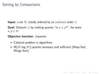
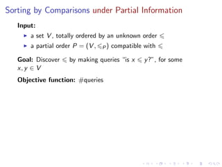
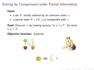
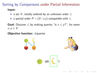
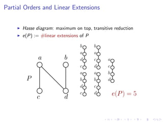
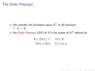
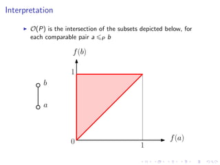
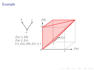
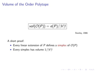
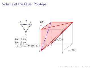
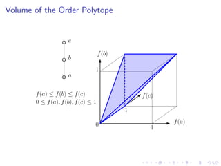
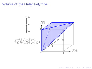
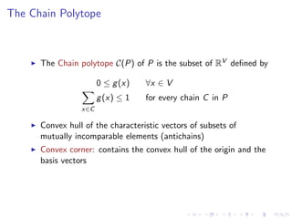
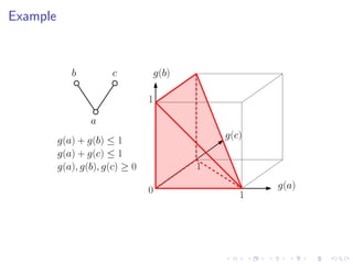
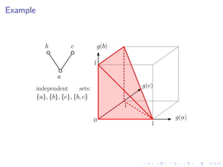
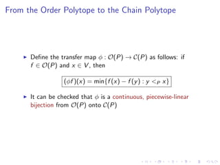
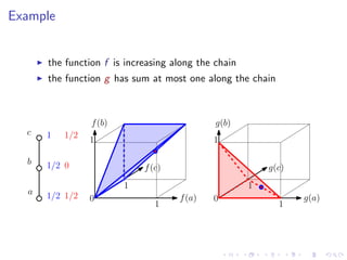
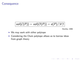
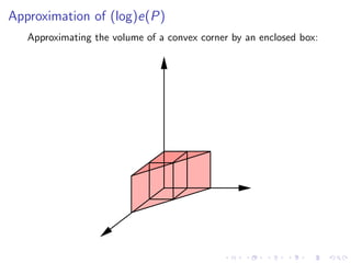
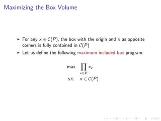
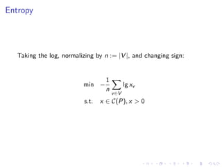
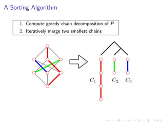
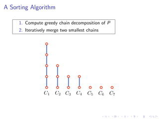
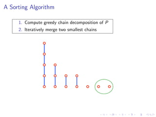
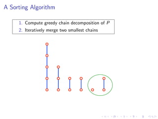
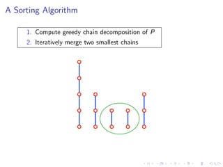
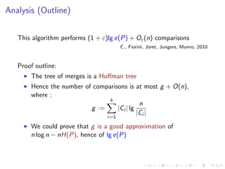
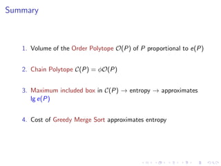
The document discusses sorting algorithms based on comparisons in the context of partial information, specifically focusing on the concept of linear extensions of partial orders. It explores the relationship between the order polytope and chain polytope, proposing an approximation method for calculating the volume of these polytopes which aids in efficient sorting algorithm development. Key findings include the establishment of a framework for approximating the number of linear extensions of a partial order, indicating potential applications in various fields.

1. Sorting
and
a Tale of Two Polytopes
Jean Cardinal
ULB, Brussels, Belgium
Algorithms & Permutations, Paris, 2012

2. Sorting by Comparisons
Input: a set V , totally ordered by an unknown order
Goal: Discover by making queries “is x y ?”, for some
x, y ∈ V
Objective function: #queries
Calssical problem in algorithms
Θ(|V | log |V |) queries necessary and sufficient (Heap Sort,
Merge Sort)

3. Sorting by Comparisons under Partial Information
Input:
a set V , totally ordered by an unknown order
a partial order P = (V , P) compatible with
Goal: Discover by making queries “is x y ?”, for some
x, y ∈ V
Objective function: #queries

4. Sorting by Comparisons under Partial Information
Input:
a set V , totally ordered by an unknown order
a partial order P = (V , P) compatible with
Goal: Discover by making queries “is x y ?”, for some
x, y ∈ V
Objective function: #queries

5. Sorting by Comparisons under Partial Information
Input:
a set V , totally ordered by an unknown order
a partial order P = (V , P) compatible with
Goal: Discover by making queries “is x y ?”, for some
x, y ∈ V
Objective function: #queries

6. Sorting by Comparisons under Partial Information
Input:
a set V , totally ordered by an unknown order
a partial order P = (V , P) compatible with
Goal: Discover by making queries “is x y ?”, for some
x, y ∈ V
Objective function: #queries
OR ?

7. Sorting by Comparisons under Partial Information
Input:
a set V , totally ordered by an unknown order
a partial order P = (V , P) compatible with
Goal: Discover by making queries “is x y ?”, for some
x, y ∈ V
Objective function: #queries
OR ?

8. Sorting by Comparisons under Partial Information
Input:
a set V , totally ordered by an unknown order
a partial order P = (V , P ) compatible with
Goal: Discover by making queries “is x y ?”, for some
x, y ∈ V
Objective function: #queries

9. Sorting by Comparisons under Partial Information
Input:
a set V , totally ordered by an unknown order
a partial order P = (V , P) compatible with
Goal: Discover by making queries “is x y ?”, for some
x, y ∈ V
Objective function: #queries
OR ?

10. Sorting by Comparisons under Partial Information
Input:
a set V , totally ordered by an unknown order
a partial order P = (V , P ) compatible with
Goal: Discover by making queries “is x y ?”, for some
x, y ∈ V
Objective function: #queries
OR ?

11. Sorting by Comparisons under Partial Information
Input:
a set V , totally ordered by an unknown order
a partial order P = (V , P ) compatible with
Goal: Discover by making queries “is x y ?”, for some
x, y ∈ V
Objective function: #queries

12. Partial Orders and Linear Extensions
Hasse diagram: maximum on top, transitive reduction
e(P) := #linear extensions of P
b b
a a
a b d c a
c d c
a a b
P b b d
d c
c d
c d e(P ) = 5

13. Lower Bound
Every comparison-based sorting algorithm can be forced to do at
least
lg e(P)
comparisons.

14. Balanced Pairs
Does there always exist a comparison that ”splits” the set of linear
extensions into roughly equal part?
1/3 − 2/3 conjecture: In any partial order P, there exists a
pair of elements a, b such that the fraction of linear extensions
having a < b is between 1/3 and 2/3
Proved for smaller values
Brightwell, Felsner, and Trotter, 1995 – Brightwell, 1999

15. A Counting Issue
Computing e(P), or computing the fraction of linear
extensions in which a < b for some pair a, b are #P-Complete
problems Brightwell and Winkler, 1991
Goal of this talk:
Insights into approximations of lg e(P) that will eventually
yield efficient sorting algorithms

16. Plan
The Order Polytope O(P) of P and how it relates to lg e(P)
The Chain Polytope C(P) and how it relates to O(P)
Approximating lg e(P) using the graph entropy and how it
relates to the two polytopes
A sorting algorithm

17. The Order Polytope
We consider the Euclidean space RV of all functions
f :V →R
the Order Polytope O(P) of P is the subset of RV defined by:
0 ≤ f (x) ≤ 1 ∀x ∈ V
f (x) ≤ f (y ) if x P y

18. Interpretation
O(P) is the intersection of the subsets depicted below, for
each comparable pair a P b
f (b)
1
b
a
0 f (a)
1

19. Example
b c f (b)
1
a
f (a) ≤ f (b) f (c)
f (a) ≤ f (c)
0 ≤ f (a), f (b), f (c) ≤ 1 1
0 f (a)
1

20. Volume of the Order Polytope
vol(O(P)) = e(P)/|V |!
Stanley, 1986
A short proof:
Every linear extension of P defines a simplex of O(P)
Every simplex has volume 1/|V |!

21. Volume of the Order Polytope
b ?c c f (b)
1
a
a
f (a) ≤ f (b) f (c)
f (a) ≤ f (c)
0 ≤ f (a), f (b), f (c) ≤ 1 1
0 f (a)
1

22. Volume of the Order Polytope
c
f (b)
b
1
a
f (a) ≤ f (b) ≤ f (c) f (c)
0 ≤ f (a), f (b), f (c) ≤ 1
1
0 f (a)
1

23. Volume of the Order Polytope
b
f (b)
c
1
a
f (a) ≤ f (c) ≤ f (b) f (c)
0 ≤ f (a), f (b), f (c) ≤ 1
1
0 f (a)
1

24. The Chain Polytope
The Chain polytope C(P) of P is the subset of RV defined by
0 ≤ g (x) ∀x ∈ V
g (x) ≤ 1 for every chain C in P
x∈C
Convex hull of the characteristic vectors of subsets of
mutually incomparable elements (antichains)
Convex corner: contains the convex hull of the origin and the
basis vectors

25. Example
b c g(b)
1
a
g(c)
g(a) + g(b) ≤ 1
g(a) + g(c) ≤ 1
g(a), g(b), g(c) ≥ 0 1
0 g(a)
1

26. Example
b c g(b)
1
a
independent sets: g(c)
{a}, {b}, {c}, {b, c}
1
0 g(a)
1

27. From the Order Polytope to the Chain Polytope
Define the transfer map φ : O(P) → C(P) as follows: if
f ∈ O(P) and x ∈ V , then
(φf )(x) = min{f (x) − f (y ) : y <P x}
It can be checked that φ is a continuous, piecewise-linear
bijection from O(P) onto C(P)

28. Example
the function f is increasing along the chain
the function g has sum at most one along the chain
f (b) g(b)
c 1 1/2
1 1
b 1/2 0 f (c) g(c)
1 1
a 1/2 1/2 0 f (a) 0 g(a)
1 1

29. Consequence
vol(C(P)) = vol(O(P)) = e(P)/|V |!
Stanley, 1986
We may work with either polytope
Considering the Chain polytope allows us to borrow ideas
from graph theory

30. Approximation of (log)e(P)
Approximating the volume of a convex corner by an enclosed box:

31. Maximizing the Box Volume
For any x ∈ C(P), the box with the origin and x as opposite
corners is fully contained in C(P)
Let us define the following maximum included box program:
max xv
v ∈V
s.t. x ∈ C(P)

32. Entropy
Taking the log, normalizing by n := |V |, and changing sign:
1
min − lg xv
n
v ∈V
s.t. x ∈ C(P), x > 0

33. Entropy
Let us give it a name:
1
H(P) = min − lg xv
n
v ∈V
s.t. x ∈ C(P), x > 0
Special case of the Graph Entropy K¨rner, 1973
o
Applications to data compression, Boolean formulas,
optimization

34. Entropy
For P a total order, C(P) is the convex hull of the basis
vectors only
We set xv = 1/n ∀v ∈ V , and obtain H(P) = log n
For P an empty order, C(P) is the unit cube
We set xv = 1 ∀v ∈ V , and obtain H(P) = 0
Intuitively, H(P) measures the quantity of information
contained in P

35. Approximation
Let x define the optimal box
The volume of the box is bounded by that of the polytope:
xv ≤ e(P)/n!
v ∈V
1
H(P) = − log xv
n
v ∈V
n log n − nH(P) ≤ lg e(P) + 1.443n

36. Approximation
In fact, we can show that
lg e(P) = Θ(n log n − nH(P))
Kahn and Kim, 1992
Furthermore, computing H(P) is a convex programming
problem, that can be solved in polynomial time
Hence we get a polynomial time constant-factor
approximation algorithm for the sorting lower bound lg e(P)

37. A Sorting Algorithm
1. Compute greedy chain decomposition of P
2. Iteratively merge two smallest chains
C1 C2 C3

38. A Sorting Algorithm
1. Compute greedy chain decomposition of P
2. Iteratively merge two smallest chains
C1 C2 C3 C4 C5 C6 C7

39. A Sorting Algorithm
1. Compute greedy chain decomposition of P
2. Iteratively merge two smallest chains

40. A Sorting Algorithm
1. Compute greedy chain decomposition of P
2. Iteratively merge two smallest chains

41. A Sorting Algorithm
1. Compute greedy chain decomposition of P
2. Iteratively merge two smallest chains

42. A Sorting Algorithm
ETC.

43. Analysis (Outline)
This algorithm performs (1 + ε)lg e(P) + Oε (n) comparisons
C., Fiorini, Joret, Jungers, Munro, 2010
Proof outline:
The tree of merges is a Huffman tree
Hence the number of comparisons is at most g + O(n),
where :
k
n
g := |Ci | lg
|Ci |
i=1
We could prove that g is a good approximation of
n log n − nH(P), hence of lg e(P)

44. Summary
1. Volume of the Order Polytope O(P) of P proportional to e(P)
2. Chain Polytope C(P) = φO(P)
3. Maximum included box in C(P) → entropy → approximates
lg e(P)
4. Cost of Greedy Merge Sort approximates entropy

45. Extending the Scope
The graph entropy framework provides efficient algorithms for
approximating the number of linear extensions of a partial
order
Can it be used for other applications?
Can it be used to approximate other quantities?

46. Thank You!

47. Pointers: Stanley’s map
R. P. Stanley.
Two poset polytopes.
Discrete Comput. Geom., 1:9–23, 1986.

48. Pointers: Counting Linear Extensions
G. R. Brightwell and P. Winkler.
Counting linear extensions.
Order, 8(3):225–242, 1991.

49. Pointers: Sorting
M. L. Fredman.
How good is the information theory bound in sorting?
Theor. Comput. Sci., 1(4):355–361, 1976.
N. Linial.
The information-theoretic bound is good for merging.
SIAM J. Comput., 13(4):795–801, 1984.
J. Kahn and M. E. Saks.
Balancing poset extensions.
Order, 1:113–126, 1984.
J. Kahn and N. Linial.
Balancing extensions via Brunn-Minkowski.
Combinatorica, 11:363–368, 1991.
G. R. Brightwell.
Balanced pairs in partial orders.
Discrete Mathematics, 201(1–3):25–52, 1999.

50. Pointers: Entropy
J. K¨rner.
o
Coding of an information source having ambiguous alphabet
and the entropy of graphs.
In Transactions of the 6th Prague Conference on Information
Theory, pages 411–425, 1973.
G. Simonyi.
Graph entropy: a survey.
In Combinatorial optimization (New Brunswick, NJ,
1992–1993), volume 20 of DIMACS Ser. Discrete Math.
Theoret. Comput. Sci., pages 399–441. Amer. Math. Soc.,
Providence, RI, 1995.

51. Pointers: Sorting and Entropy
J. Kahn and J. H. Kim.
Entropy and sorting.
J. Comput. Syst. Sci., 51(3):390–399, 1995.
A. C.-C. Yao.
Graph entropy and quantum sorting problems.
In STOC’04: 36th Annual ACM Symposium on Theory of
Computing, pages 112–117, 2004.
J. C., S. Fiorini, G. Joret, R. Jungers, and J. I. Munro.
An efficient algorithm for partial order production.
In STOC ’09: 41st ACM Symposium on Theory of Computing,
2009.
J. C., S. Fiorini, G. Joret, R. Jungers, and J. I. Munro.
Sorting under Partial Information (without the Ellipsoid
Algorithm).
In STOC ’10: 42nd ACM Symposium on Theory of
Computing, 2010.