The document discusses representations and operations on polynomials. It describes how polynomials can be represented as lists of coefficients. It also explains how to perform basic polynomial operations like evaluation, addition, multiplication, division, and finding the greatest common divisor (GCD) of two polynomials. Horner's method and the Euclidean algorithm are key algorithms discussed for efficiently evaluating and finding the GCD of polynomials.

1. Polynomials
Jordi Cortadella
Department of Computer Science
Outline
• How to represent a polynomial?
• Evaluation of a polynomial.
• Basic operations: sum, product and division.
• Greatest common divisor.
Introduction to Programming © Dept. CS, UPC 2
Representation of polynomials
Introduction to Programming © Dept. CS, UPC 3
A list of coefficients
Properties of the representation:
• 𝑎𝑛 ≠ 0 (the topmost element is not zero).
• 𝑃 𝑥 = 0 is represented with an empty vector.
𝑃 𝑥 = 𝑎𝑛𝑥𝑛 + 𝑎𝑛−1𝑥𝑛−1 + ⋯ + 𝑎1𝑥 + 𝑎0
𝑛 𝑛 − 1 ⋯ 1 0
𝑎𝑛 𝑎𝑛−1 ⋯ 𝑎1 𝑎0
Polynomial evaluation (Horner’s scheme)
• Design a function that evaluates the value of a
polynomial.
• A polynomial of degree 𝑛 can be efficiently
evaluated using Horner’s algorithm:
𝑃 𝑥 = 𝑎𝑛𝑥𝑛 + 𝑎𝑛−1𝑥𝑛−1 + ⋯ + 𝑎1𝑥 + 𝑎0 =
(⋯ ((𝑎𝑛𝑥 + 𝑎𝑛−1)𝑥 + 𝑎𝑛−2)𝑥 + ⋯ )𝑥 + 𝑎0
• Example:
3𝑥3
− 2𝑥2
+ 𝑥 − 4 = 3𝑥 − 2 𝑥 + 1 𝑥 − 4
Introduction to Programming © Dept. CS, UPC 4

2. Polynomial evaluation (Horner’s scheme)
Introduction to Programming © Dept. CS, UPC 5
3𝑥3
− 2𝑥2
+ 𝑥 − 4
3 𝑥 − 2 𝑥 + 1
3 𝑥 − 2 𝑥 + 1 𝑥 − 4
3 𝑥 − 2
3
Polynomial evaluation (Horner’s scheme)
def poly_eval(P, x):
"""Returns the evaluation of P(x)"""
r = 0
# Evaluates the polynomial using Horner's scheme
# The coefficients are visited from highest to lowest
for i in range(len(P)-1, -1, -1):
r = r*x + P[i]
return r
Introduction to Programming © Dept. CS, UPC 6
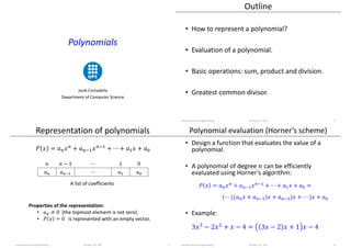
Product of polynomials
Example:
Introduction to Programming © Dept. CS, UPC 7
def poly_mul(P, Q):
"""Returns P*Q"""
𝑃 𝑥 = 2𝑥3 + 𝑥2 − 4
𝑄 𝑥 = 𝑥2
− 2𝑥 + 3
𝑃 ⋅ 𝑄 𝑥 = 2𝑥5 + −4 + 1 𝑥4 + 6 − 2 𝑥3 + −4 + 3 𝑥2 + 8𝑥 − 12
𝑃 ⋅ 𝑄 𝑥 = 2𝑥5
− 3𝑥4
+ 4𝑥3
− 𝑥2
+ 8𝑥 − 12
Product of polynomials
• Key point:
Given 𝑃 𝑥 = 𝑎𝑛𝑥𝑛 + 𝑎𝑛−1𝑥𝑛−1 + ⋯ + 𝑎1𝑥 + 𝑎0
and 𝑄 𝑥 = 𝑏𝑚𝑥𝑚 + 𝑏𝑚−1𝑥𝑚−1 + ⋯ + 𝑏1𝑥 + 𝑏0,
what is the coefficient 𝑐𝑖 of 𝑥𝑖
in (𝑃 ⋅ 𝑄)(𝑥)?
• The product 𝑎𝑖𝑥𝑖
⋅ 𝑏𝑗𝑥𝑗
must be added to the term
with 𝑥𝑖+𝑗
.
• Idea: for every 𝑖 and 𝑗, add 𝑎𝑖 ⋅ 𝑏𝑗 to the (𝑖 + 𝑗)-th
coefficient of the product.
Introduction to Programming © Dept. CS, UPC 8

3. Product of polynomials
Introduction to Programming © Dept. CS, UPC 9
2 -1 9 -5 10 -3
𝑥5
𝑥4
𝑥3
𝑥2
𝑥1
𝑥0
𝑥3 𝑥2 𝑥1 𝑥0
2 -1 3
1 0 3 -1
×
2 6
-1
0 -2
0 -3 1
3 0 9 -3
+
Product of polynomials
def poly_mul(P, Q):
"""Returns P*Q"""
# Special case for a polynomial of size 0
if len(P) == 0 or len(Q) == 0:
return []
R = [0]*(len(P)+len(Q)-1) # list of zeros
for i in range(len(P)):
for j in range(len(Q)):
R[i+j] += P[i]*Q[j]
return R
Introduction to Programming © Dept. CS, UPC 10
Sum of polynomials
• Note that over the real numbers,
degree 𝑃 ⋅ 𝑄 = degree 𝑃 + degree(𝑄)
(except if 𝑃 = 0 or 𝑄 = 0).
So we know the size of the result vector a priori.
• This is not true for the polynomial sum, e.g.,
degree 𝑥 + 5 + −𝑥 − 1 = 0
Introduction to Programming © Dept. CS, UPC 11
Sum of polynomials
A function to normalize a polynomial might be useful in
some algorithms, i.e., remove the leading zeros to
guarantee the most significant coefficient is not zero.
Introduction to Programming © Dept. CS, UPC 12
def poly_normalize(P):
"""Resizes the polynomial to guarantee that the
leading coefficient is not zero."""
while len(P) > 0 and P[-1] == 0:
P.pop(-1)

4. Sum of polynomials
def poly_add(P, Q):
"""Returns P+Q"""
if len(Q) > len(P): # guarantees len(P) >= len(Q)
P, Q = Q, P
# Adds the coefficients up to len(Q)
R = []
for i in range(len(Q)):
R.append(P[i]+Q[i])
R += P[i+1:] # appends the remaining coefficients of P
poly_normalize(R)
return R
Introduction to Programming © Dept. CS, UPC 13
P
Q
Euclidean division of polynomials
• For every pair of polynomials 𝐴 and 𝐵, such that
𝐵 ≠ 0, find 𝑄 and 𝑅 such that
𝐴 = 𝐵 ∙ 𝑄 + 𝑅
and degree 𝑅 < degree(𝐵).
𝑄 and 𝑅 are the only polynomials satisfying this
property.
• Classical algorithm: Polynomial long division.
Introduction to Programming © Dept. CS, UPC 14
Polynomial long division
def poly_div(A, B):
"""Returns the quotient (Q) and the remainder (R)
of the Euclidean division A/B. They are returned
as a tuple (Q, R)"""
Introduction to Programming © Dept. CS, UPC 15
A B R
Q A B R
Q
Polynomial long division
Introduction to Programming © Dept. CS, UPC 16
def poly_div(A, B):
"""Returns the quotient (Q) and the remainder (R)
of the Euclidean division A/B. They are returned
as a tuple (Q, R)"""

5. A B R
Q
Polynomial long division
Introduction to Programming © Dept. CS, UPC 17
def poly_div(A, B):
"""Returns the quotient (Q) and the remainder (R)
of the Euclidean division A/B. They are returned
as a tuple (Q, R)"""
A B R
Q
Polynomial long division
Introduction to Programming © Dept. CS, UPC 18
def poly_div(A, B):
"""Returns the quotient (Q) and the remainder (R)
of the Euclidean division A/B. They are returned
as a tuple (Q, R)"""
A B R
Q
Polynomial long division
Introduction to Programming © Dept. CS, UPC 19
def poly_div(A, B):
"""Returns the quotient (Q) and the remainder (R)
of the Euclidean division A/B. They are returned
as a tuple (Q, R)"""
A B R
Q
Polynomial long division
Introduction to Programming © Dept. CS, UPC 20
def poly_div(A, B):
"""Returns the quotient (Q) and the remainder (R)
of the Euclidean division A/B. They are returned
as a tuple (Q, R)"""

6. A B R
Q
Polynomial long division
Introduction to Programming © Dept. CS, UPC 21
def poly_div(A, B):
"""Returns the quotient (Q) and the remainder (R)
of the Euclidean division A/B. They are returned
as a tuple (Q, R)"""
Polynomial long division
Introduction to Programming © Dept. CS, UPC 22
A B R
Q
def poly_div(A, B):
"""Returns the quotient (Q) and the remainder (R)
of the Euclidean division A/B. They are returned
as a tuple (Q, R)"""
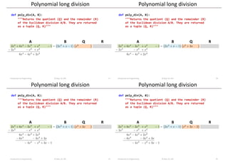
Polynomial long division
Introduction to Programming © Dept. CS, UPC 23
2 6 -3 1 0 -1 2 0 1 -1
1 3 -2
5 4 3 2 1 0 3 2 1 0
2 1 0
R: B:
Q:
6 -4 2 0 -1
-4 -1 3 -1
-1 5 -3
A
Invariant: A = BQ+R
Polynomial long division
def poly_div(A, B):
"""Returns the quotient (Q) and the remainder (R) of the
Euclidean division A/B. They are returned as a tuple (Q, R)"""
R = A[:] # copy of A
if len(A) < len(B):
return [], R
Q = [0]*(len(A)-len(B)+1)
# For each digit of Q
for iQ in range(len(Q)-1, -1, -1):
Q[iQ] = R[-1]/B[-1]
R.pop(-1)
for k in range(len(B)-1):
R[k+iQ] -= Q[iQ]*B[k]
poly_normalize(R)
return Q, R
Introduction to Programming © Dept. CS, UPC 24
iQ
k
k+iQ

7. GCD of two polynomials
Introduction to Programming © Dept. CS, UPC 25
Example:
Re-visiting Euclidean algorithm for gcd
# gcd(a, 0) = a
# gcd(a, b) = gcd(b, a%b)
def gcd(a, b):
"""Returns gcd(a, b)"""
while b > 0:
a, b = b, a%b
return a
For polynomials:
• a and b are polynomials.
• a%b is the remainder of
the Euclidean division.
Introduction to Programming © Dept. CS, UPC 26
Euclidean algorithm for gcd
def poly_gcd(A, B):
"""Returns gcd(A, B)"""
while len(B) > 0:
Q, R = poly_div(A, B)
A, B = B, R
# Converts to monic polynomial (e.g., 3x-6  x-2)
c = A[–1]
for i in range(len(A)):
A[i] /= c
return A
Introduction to Programming © Dept. CS, UPC 27
Euclidean algorithm for gcd
monic polynomial
Introduction to Programming © Dept. CS, UPC 28

8. Conclusions
• Polynomials are used very often in numerical
analysis.
• Polynomial functions have nice properties:
continuous and simple derivatives and
antiderivatives.
• There are simple root-finding algorithms to
find approximations of the roots.
Introduction to Programming © Dept. CS, UPC 29