Download to read offline


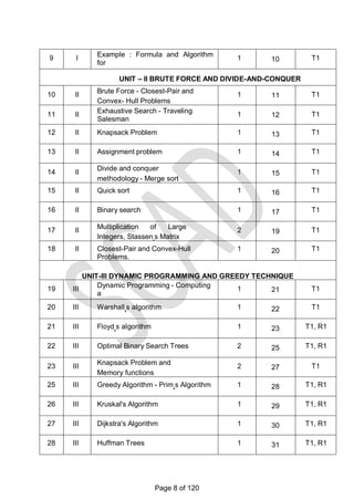

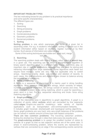
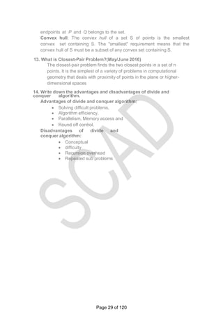
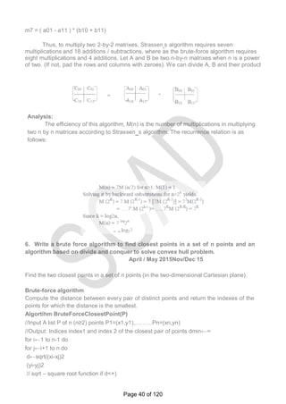
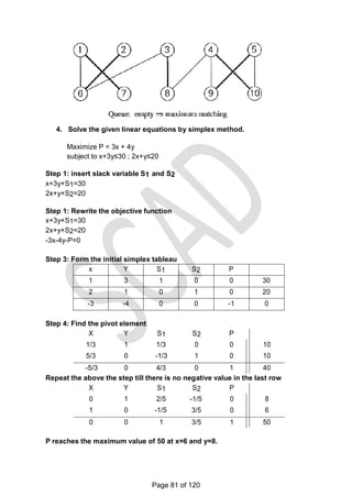
![5. With an algorithm explain in detail about the linear search. Give its
efficiency.
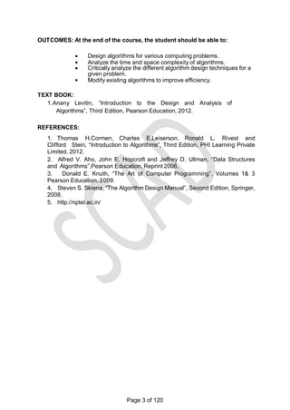
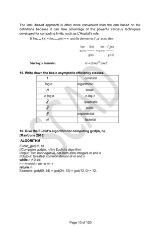
SEQUENTIAL SEARCH
Sequential Search searches for the key value in the given set of items
sequentially and returns the position of the key value else returns -1.
Algorithm sequentialsearch(A[0….n-1],K)
//Searches for a given array by sequential search
//Input: An array A[0….n-1} and a search key K
// the index of the first element of A that matches K or -1 if there are no matching
elements i←0
while i<n and A[i]≠K do
i←i+1 if i<n return i else return -1
Analysis:
For sequential search, best-case inputs are lists of size n with their first
elements equal to a search key; accordingly, Cbw(n) = 1.
Average Case Analysis:
The standard assumptions are that :
a. the probability of a successful search is equal top (0 <=p<-=1) and
b. the probability of the first match occurring in the ith position of the list is
the same for every i. Under these assumptions- the average number of key
comparisons Cavg(n) is found as
follows.
In the case of a successful search, the probability of the first
match occurring in the i th position of the list is p / n for every i,
and the number of comparisons made by the algorithm in such a
situation is obviously i.
6. Explain in detail about mathematical analysis of recursive algorithm
MATHEMATICAL ANALYSIS FOR RECURSIVE ALGORITHMS
General Plan for Analysing the Time Efficiency of Recursive Algorithms:
1. Decide on a parameter (or parameters) indicating an input’s size.
2. Identify the algorithm‘s basic operation.
Page 23 of 120](https://image.slidesharecdn.com/cs6402-scad-msm-191208081445/85/Cs6402-scad-msm-23-320.jpg)
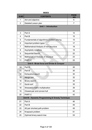
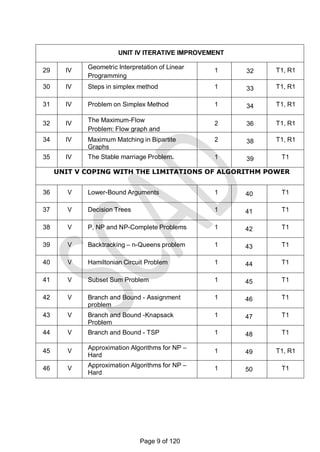
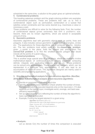
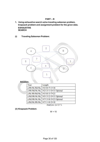
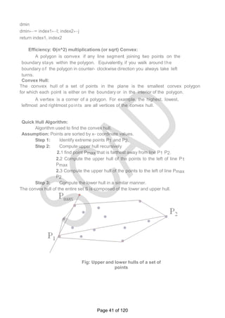
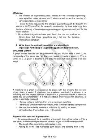
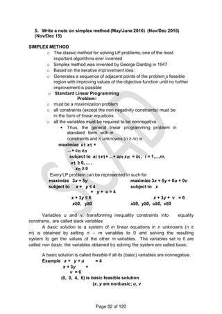
![PART-C
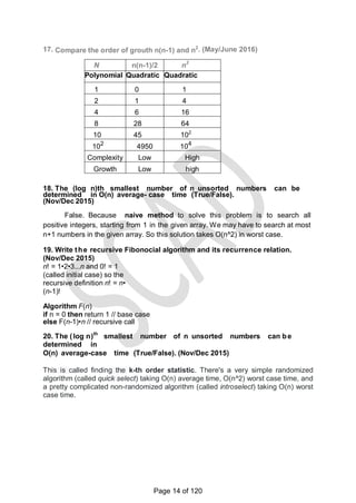
1. Give an algorithm to check whether all the Elements in a given array
of n elements are distinct. Find the worst case complexity of the same.
Element uniqueness problem: check whether all the Elements in a given
array of n elements are distinct.
ALGORITHM UniqueElements(A[0..n − 1])
//Determines whether all the elements in a given
array are distinct
//Input: An array A[0..n − 1]
//Output: Returns ―true‖ if all the elements in A are distinct and ―false‖
otherwise
for i ←0 to n − 2 do
for j ←i + 1 to n − 1 do
if A[i]= A[j ] return false
return true
Worst case Algorithm analysis
The natural measure of the input‗s size here is again n (the number
of elements in the array).
Since the innermost loop contains a single operation (the comparison
of two elements),
we
should consider it as the algorithm‗s basic operation.
The number of element comparisons depends not only on n but also
on whether there are equal elements in the array and, if there are,
which array positions they occupy. We will limit our investigation to
the worst case only.
One comparison is made for each repetition of the innermost loop,
i.e., for each value of the loop variable j between its limits i + 1 and n − 1;
this is repeated for each value of the outer loop, i.e., for each value of the
loop variable i between its limits 0 and n − 2.
2. Give the recursive algorithm which finds the number of binary
digits in the binary representation of a positive decimal integer. Find
the recurrence relation and complexity. (May/June 2016)
Page 25 of 120](https://image.slidesharecdn.com/cs6402-scad-msm-191208081445/85/Cs6402-scad-msm-25-320.jpg)

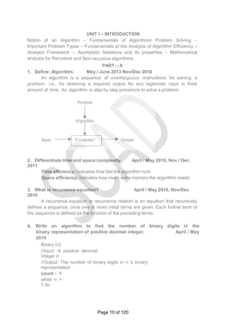
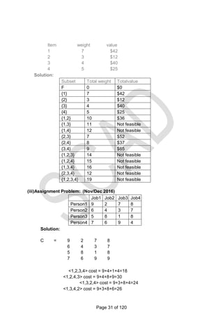
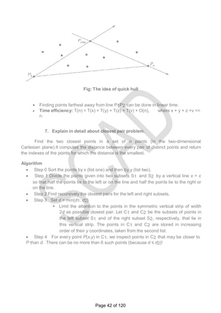
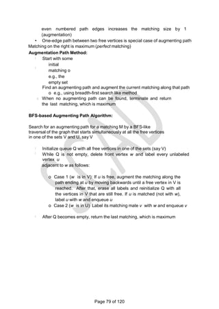
![• Weights: w1 w2 … wn
• Values: v1 v2 … vn
• A knapsack of capacity W
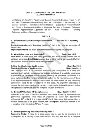
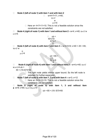
7. Give the control abstraction of divide and conquer techniques. Nov
/Dec 2012,13
Control abstraction for recursive divide and conquer, with
problem instance P
divide_and_conquer ( P )
{
divide_and_conquer ( P2 ),
...
divide_and_conquer ( Pk ) ) );
}
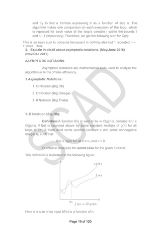
8. Differentiate linear search and binary search. Nov / Dec 2014
Linear search: Linear Search or Sequential Search searches for
the key value in the given set of items sequentially and returns the position
of the key value else returns -1. Binary search: Binary search is a
remarkably efficient algorithm for searching in a sorted array. It works by
comparing a search key K with the arrays middle element A[m]. If they
match the algorithm stops; otherwise the same operation is repeated
recursively for the first half of the array if K < A[m] and the second half if K >
A[m].
9. Derive the complexity for binary search algorithm. April / May 2012,15
Nov/Dec 2016
10.. Distinguish between quick sort and merge sort. Nov/ Dec 2011
Merge
Sort
Quick
SortFor merge sort the arrays are
partitioned
according to their position
In quick sort the arrays are
partitioned
according to the element values.
11. Give the time complexity of merge sort.
Cworst(n) = 2Cworst(n/2) + n- 1 for n> 1, Worst(1)=0
Cworst(n) € Θ(n log n) (as per master‗s theorem)
12. Define: Convex and Convex hull.
Convex: A set of points (finite or infinite) in the plane is called convex if
for any two points P and Q in the set, the entire line segment with the
Page 28 of 120](https://image.slidesharecdn.com/cs6402-scad-msm-191208081445/85/Cs6402-scad-msm-28-320.jpg)
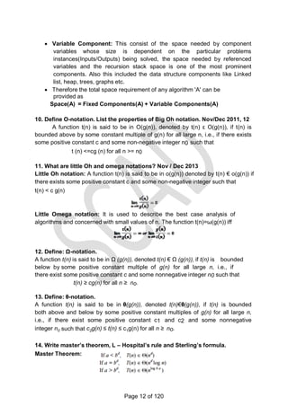
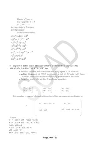
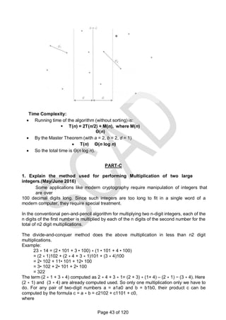
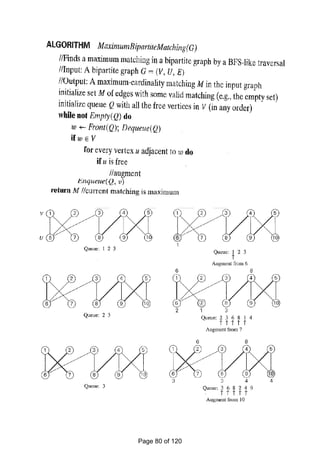
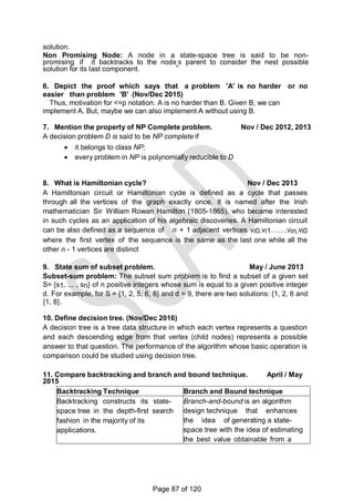
![<1,4,2,3> cost = 9+7+8+9=33
<1,4,3,2> cost = 9+7+1+6=23
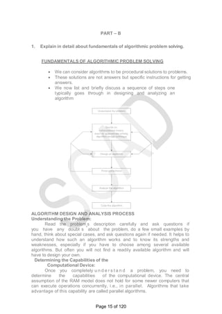
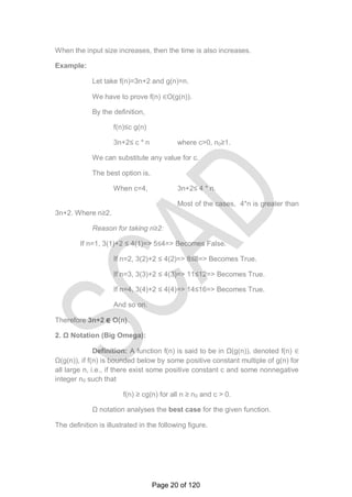
2. Explain the merge sort using divide and conquer technique give an
example. April / May 2010,May/June 2016
Devise an algorithm to perform merge sort.
Trace the steps of merge sort algorithm for the elements 8, 3, 2, 9,
7, 1, 5, 4 and also compute its time complexity.
MERGE SORT
o It is a perfect example of divide-and-conquer.
o It sorts a given array A [0..n-1] by dividing it into two halves
A[0…(n/2-1)] and A[n/2…n-1], sorting each of them recursively
and then merging the two smaller sorted arrays into a single sorted
one.
Algorithm for merge sort:
//Input: An array A [0…n-1] of
orderable elements //Output:
Array A [0..n-1] sorted in
increasing order
if n>1
Copy A[0…(n/2-1)] to
B[0…(n/2-1)] Copy
A[n/2…n-1] to
C[0…(n/2-1)] Merge
sort (B[0..(n/2-1)]
Merge sort (C[0..(n/2-
1)] Merge (B,C,A)
Merging process:
The merging of two sorted arrays can be done as follows:
o Two pointers are initialized to point to first elements of the arrays
being merged.
o Then the elements pointed to are compared and the smaller of them
is added to a new array being constructed;
o After that, that index of that smaller element is incremented to
point to its immediate successor in the array it was copied from.
This operation is continued until one of the two given arrays are
exhausted then the remaining elements of the other array are
copied to the end of the new array.
Algorithm for merging:
Algorithm Merge (B[0…P-1], C[0…q-1], A[0…p + q-1])
//Merge two sorted arrays into one sorted array.
//Input: Arrays B[0..p-1] and C[0…q-1] both sorted
//Output: Sorted Array A [0…p+q-1] of the elements of B & C
i = 0; j = 0; k = 0
Page 32 of 120](https://image.slidesharecdn.com/cs6402-scad-msm-191208081445/85/Cs6402-scad-msm-32-320.jpg)
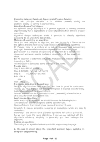
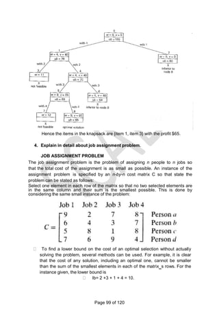
![while i < p and j < q do if B[i] ≤ C[j]
A[k] = B[i]; i = i+1
if i=p
else
k =k+1
A[k] = B[j]; j = j+1
copy C[j..q-1] to A[k..p+q-1]
else
copy B[i..p-1] to A[k..p+q-1]
Example:
Page 33 of 120](https://image.slidesharecdn.com/cs6402-scad-msm-191208081445/85/Cs6402-scad-msm-33-320.jpg)
![3. Explain the binary search with suitable example. Nov/ Dec 2011 (Nov/Dec
15) Write an algorithm to perform binary search on a sorted list of elements
and analyze the algorithm. April / May 2011
BINARY SEARCH
It is an efficient algorithm for searching in a sorted array. It is an example for
divide and conquer technique.
Working of binary search:
It works by comparing a search key k with the array‘s middle element A [m].
If they match, the algorithm stops; otherwise the same operation is
repeated recursively for the first half of the array if K < A (m) and for the
second half if K > A (m).
K
A [0] … A [m – 1] A [m] A [m+1] …. A [n-1]
Search here if K < A (m) Search here if K > A
(m)
Example:
Given set of elements
3 14 27 31 42 55 70 81 98
Search key: K=55
The iterations of the algorithm are given as:
A [m] = K, so the algorithm stops
Binary search can also implemented as a nonrecursive
algorithm. Algorithm Binarysearch(A[0..n-1], k)
// Implements nonrecursive binarysearch
// Input: An array A[0..n-1] sorted in ascending order and a search key k
// Output: An index of the array‗s element that is equal to k or -1 if there is no such element
l←0;
r←n-1
while l ≤ r do
m←[(l+r)/2]
if k = A[m] return m
else if k < A[m] r←m-1
else l←m+1
Page 34 of 120](https://image.slidesharecdn.com/cs6402-scad-msm-191208081445/85/Cs6402-scad-msm-34-320.jpg)
![return -1
Analysis:
The efficiency of binary search is to count the number of times the search key is
compared with an element of the array.
For simplicity, three-way comparisons are considered. This assumes that
after one comparison of K with A [M], the algorithm can determine whether K is smaller,
equal to, or larger than A [M]. The comparisons not only depend on ‗n‗ but also the
particular instance of the problem.
The worst case comparison Cw (n) includes all arrays that do not contain a search
key, after one comparison the algorithm considers the half size of the array.Cw (n) = Cw
(n/2) + 1 for n > 1, Cw (1) = 1 --------------------- eqn(1)
To solve such recurrence equations, assume that n = 2k to obtain the solution.
Cw ( k) = k +1 = log2n+1
For any positive even number n, n = 2i, where I > 0. now the LHS of eqn (1) is:
Cw (n) = [ log2n]+1 = [ log22i]+1 = [ log 22 + log2i] + 1 = ( 1 + [log2i]) + 1
= [ log2i] +2
The R.H.S. of equation (1) for n = 2 i is
Cw [n/2] + 1 = Cw [2i / 2] + 1
= Cw (i) + 1
= ([log2 i] + 1) + 1
= ([log2 i] + 2
Since both expressions are the same, the assertion is proved.
The worst – case efficiency is in θ (log n) since the algorithm reduces the size of the
array remained as about half the size, the numbers of iterations needed to reduce the initial
size n to the final size 1 has to be about log2n. Also the logarithmic functions grow so
slowly that its values remain small even for very large values of n.
The average-case efficiency is the number of key comparisons made which is
slightly smaller than the worst case.
More accurately, . e.Cavg (n) ≈ log2n
for successful search iCavg (n) ≈ log2n –1
for unsuccessful search Cavg (n) ≈ log2n + 1
3. Explain in detail about quick sort. (Nov/Dec 2016)
QUICK SORT
Quick sort is an algorithm of choice in many situations because it is not
difficult to implement, it is a good "general purpose" sort and it consumes relatively
fewer resources during execution.
Quick Sort and divide and conquer
Page 35 of 120](https://image.slidesharecdn.com/cs6402-scad-msm-191208081445/85/Cs6402-scad-msm-35-320.jpg)
![Divide: Partition array A[l..r] into 2 sub-arrays, A[l..s-1] and A[s+1..r] such that
each element of the first array is ≤A[s] and each element of the second array is ≥
A[s]. (Computing the index of s is part of partition.)
Implication: A[s] will be in its final position in the sorted array.
Conquer: Sort the t wo s ub -a rra y s A [l...s-1] and A [s+1...r] by r e c u r s i v e
calls to quicksort Combine: No work is needed, because A[s] is already in its
correct place after the partition is done, and the two sub arrays have been sorted.
Steps in Quicksort
Select a pivot with respect to whose value we are going to divide the
sublist. (e.g., p = A[l])
Rearrange the list so that it starts with the pivot followed by a ≤ sublist
(a sublist whose elements are all smaller than or equal to the pivot)
and a ≥ sublist (a sublist whose elements are all greater than or equal
to the pivot ) Exchange the pivot with the last element in the first
sublist(i.e., ≤ sublist) – the pivot is now in its final position.
The Quicksort Algorithm
ALGORITHM Quicksort(A[l..r])
//Sorts a subarray by quicksort
//Input: A subarray A[l..r] of A[0..n-1],defined by its left and right indices l and r
//Output: The subarray A[l..r] sorted in nondecreasing
order if l < r s Partition (A[l..r]) // s is a split
position
Quicksort(A[l..s-])
Quicksort(A[s+1..r
ALGORITHM Partition (A[l ..r])
//Partitions a subarray by using its first element as a pivot
//Input: A subarray A[l..r] of A[0..n-1], defined by its left and right indices l and r
(l < r)
//Output: A partition of A[l..r], with the split position returned as this function‗s
value
P <-A[l]
i <-l; j <- r + 1;
Repeat
repeat i <- i + 1 until A[i]>=p //left-right
scan repeat j <-j – 1 until A[j] <=
p//right-left scan
if (i < j) //need to continue with the scan swap(A[i],
a[j])
Page 36 of 120](https://image.slidesharecdn.com/cs6402-scad-msm-191208081445/85/Cs6402-scad-msm-36-320.jpg)
![until i >= j //no need
to scan swap(A[l], A[j])
return j
Advantages in Quick Sort
It is in-place since it uses only a small auxiliary stack.
It requires only n log(n) time to sort n items.
It has an extremely short inner loop
This algorithm has been subjected to a thorough mathematical analysis, a
very precise statement can be made about performance issues.
.
Disadvantages in Quick Sort
It is recursive. Especially if recursion is not available, the
i mpl ementati on is extremely complicated.
It requires quadratic (i.e., n2) time in the worst-case.
It is fragile i.e., a simple mistake in the implementation can go unnoticed and
cause it to perform badly.
Efficiency of Quicksort
Based on whether the partitioning is balanced.
Best case: split in the middle — Θ (n log n)
C (n) = 2C (n/2) + Θ (n) //2 subproblems of size n/2 each
Worst case: sorted array! — Θ (n2
)
C (n) = C (n-1) + n+1 //2 subproblems of size 0 and n-1 respectively
Average case: random arrays — Θ (n log n)
Conditions:
If i< j, swap A[i] and A[j]
If I > j, partition the array after exchanging pivot and A[j] If
i=j, the value pointed is p and thus partition the array
Example:
50 30 10 90 80 20 40 70
Step 1: P = A[l]
50 30 10 90 80 20 40 70
P I j
Step2: Inrement I; A[i] < Pivot
50 30 10 90 80 20 40 70
P I j
Step 3: Decrement j; A[j]>Pivot
Page 37 of 120](https://image.slidesharecdn.com/cs6402-scad-msm-191208081445/85/Cs6402-scad-msm-37-320.jpg)
![20 30 10 40 50 80 90 70
Left sublist I Right sublist
p
10 20
The final
40 50
s
80 90
j i
50 30 10 90 80 20 40 70
P I j
Step 4: i<j; swap A[i] & A[j]
50 30 10 40 80 20 90 70
P I j
Step 5: Increment i
50 30 10 40 80 20 90 70
P I j
Step 6: Decrement j
50 30 10 40 80 20 90 70
P I j
Step 7: i<j, swap A[i] & A[j]
50 30 10 40 20 80 90 70
P I j
Step 8: Increment I, Decrement j
50 30 10 40 20 80 90 70
P j i
Step 9: i>j, swap P & A[j]
Step 10: Increment I & Decrement j for the left sublist
20 30 10 40 50 80 90 70
P i j
Step 11: i<j, swap A[i] & A[j]
20 10 30 40 50 80 90 70
P I j
Step 12: inc I, Dec j for left sublist
20 10 30 40 50 80 90 70
P j i
Step 13: i>j, swap P & A[j]
10 20 30 40 50 80
90 70 j
Step 14: inc I, Dec j for right sublist
10 20 30 40 50 80 90 70
P I j
Step 15: i<j, swap A[i] & A[j]
10 20 30 40 50 80 70 90
P I j
Step 16: inc I, Dec j for right sublist
10 20 30 40 50 80 70 90
P p j i
Step 17: i>j, Exchange P & A[j]
Page 38 of 120](https://image.slidesharecdn.com/cs6402-scad-msm-191208081445/85/Cs6402-scad-msm-38-320.jpg)
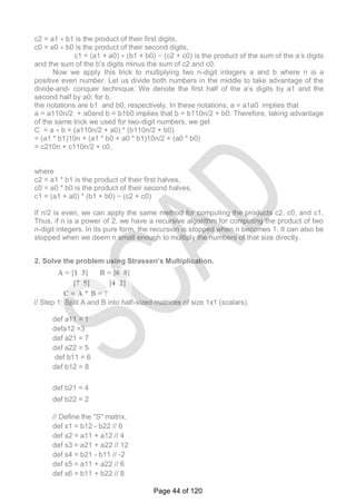
![def s7 = a12 - a22 // -2
def s8 = b21 + b22 // 6
def s9 = a11 - a21 // -6
def s10 = b11 + b12 // 14
// Define the "P" matrix.
def p1 = a11 * s1 // 6
def p2 = s2 * b22 // 8
def p3 = s3 * b11 // 72
def p4 = a22 * s4 // -10
def p5 = s5 * s6 // 48
def p6 = s7 * s8 // -12
def p7 = s9 * s10 // -84
// Fill in the resultant "C" matrix.
def c11 = p5 + p4 - p2 + p6 // 18
def c12 = p1 + p2 // 14
def c21 = p3 + p4 // 62
def c22 = p5 + p1 - p3 - p7 // 66
RESULT:
C = [ 18 14]
[ 62 66]
Page 45 of 120](https://image.slidesharecdn.com/cs6402-scad-msm-191208081445/85/Cs6402-scad-msm-45-320.jpg)
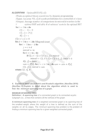
![UNIT III - DYNAMIC PROGRAMMING AND GREEDY TECHNIQUE
Computing a Binomial Coefficient – Warshall‗s and Floyd‗s algorithm – Optimal
Binary Search Trees – Knapsack Problem and Memory functions. Greedy
Technique– Prim‟s algorithm- Kruskal's Algorithm- Dijkstra's Algorithm-Huffman
Trees.
PART – A
1. What do you mean by dynamic programming? April / May 2015
Dynamic programming is an algorithm design method that can be
used when a solution to the problem is viewed as the result of sequence
of decisions. Dynamic programming is a technique for solving problems with
overlapping sub problems. These sub problems arise from a recurrence relating
a solution to a given problem with solutions to its smaller sub problems only
once and recording the results in a table from which the solution to the
original problem is obtained. It was invented by a prominent U.S
Mathematician, Richard Bellman in the 1950s.
2. List out the memory functions used under dynamic programming. April / May
2015
Let V[i,j] be optimal value of such an instance. Then
V[i,j]= max {V[i-1,j], vi + V[i-1,j- wi]} if j- wi 0
V[i-1,j] if j- wi < 0
Initial conditions: V[0,j] = 0 for j>=0 and V[i,0] = 0 for i>=0
3. Define optimal binary search tree. April / May 2010
An optimal binary search tree (BST), is a binary search tree which
provides the smallest possible search time (or expected search time) for
a given sequence of accesses (or access probabilities).
4. List out the advantages of dynamic programming. May / June 2014
Optimal solutions to sub problems are retained so as to avoid re
computing their values.
Decision sequences containing subsequences that are sub optimal are not
considered.
It definitely gives the optimal solution always.
5. State the general principle of greedy algorithm. Nov / Dec 2010
Greedy technique suggests a greedy grab of the best alternative available in the
hope that a sequence of locally optimal choices will yield a globally optimal
solution to the entire problem. The choice must be made as follows
Page 46 of 120](https://image.slidesharecdn.com/cs6402-scad-msm-191208081445/85/Cs6402-scad-msm-46-320.jpg)
![guarantees a solution with value no worst than 1/2 the optimal solution.
11. Write an algorithm to compute the binomial coefficient.
Algorithm Binomial(n,k)
//Computes C(n,k) by the dynamic programming algorithm
//Input: A pair of nonnegative integers n>=k>=0
//Output: The value of C(n,k)
for i ← 0 to n do
for j ←0 to min(i,k) do if j=0 or j=i
C[i,j] ←1
else C[i,j] ← C[i-1,j-1]+C[i-1,j]
return C[n,k]
12. Devise an algorithm to make a change using the greedy strategy.
Algorithm Change(n, D[1..m])
//Implements the greedy algorithm for the change-making problem
//Input: A nonnegative integer amount n and
// a decreasing array of coin denominations D
//Output: Array C[1..m] of the number of coins of each denomination
// in the change or the ‖no solution‖ message for i ← 1 to m do
C[i] ← n/D[i]
n ← n mod D[i]
if n = 0 return C
else return ‖no solution‖
13. What is the best algorithm suited to identify the topography for
a graph. Mention its efficiency factors. (Nov/Dec 2015)
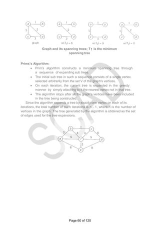
Prim and Kruskal‘s are the best algorithm suited to identify the topography of graph
14. What is spanning tree and minimum spanning tree?
Spanning tree of a connected graph G: a connected acyclic sub graph of
G that includes all of G‗s vertices
Minimum spanning tree of a weighted, connected graph G: a spanning tree
of G of the minimum total weight
15. Define the single source shortest path problem. (May/June 2016)
(Nov/Dec 2016)
Dijkstra‗s algorithm solves the single source shortest path problem of finding
shortest paths from a given vertex( the source), to all the other vertices of a
weighted graph or digraph. Dijkstra‗s algorithm provides a correct solution for a
graph with non-negative weights.
PART-B
1. Write down and explain the algorithm to solve all pair shortest path
algorithm. April / May 2010
Page 48 of 120](https://image.slidesharecdn.com/cs6402-scad-msm-191208081445/85/Cs6402-scad-msm-48-320.jpg)
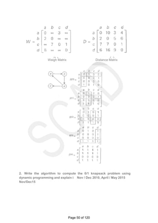
![Write and explain the algorithm to compute all pair source shortest
path using dynamic programming. Nov / Dec 2010
Explain in detail about Floyd’s algorithm. (Nov/Dec 2016)
ALL PAIR SHORTEST PATH
It is to find the distances (the length of the shortest paths) from each
vertex to all other vertices.
It‗s convenient to record the lengths of shortest paths in an n x n
matrix D called distance matrix.
It computes the distance matrix of a weighted graph with n vertices thru
a series of n x n matrices.
D0, D (1), …… D (k-1) , D (k),…… D(n)
Algorithm
//Implemnt Floyd‗s algorithm for the all-pairs shortest-paths problem
// Input: The weight matrix W of a graph
// Output: The distance matrix of the shortest paths lengths
D← w
for k ← 1 to n do
for i ← 1 to n do for j← 1 to n do
D[i,j] min {D[i,j], D[i,k] + D[k,j]}
Return D.
Example:
Page 49 of 120](https://image.slidesharecdn.com/cs6402-scad-msm-191208081445/85/Cs6402-scad-msm-49-320.jpg)
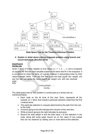
![KNAPSACK PROBLEM
Given n items of integer weights: w1 w2 … wn , values: v1 v2 … vn
and a knapsack of integer capacity W find most valuable subset of the items that
fit into the knapsack.
Consider instance defined by first i items and capacity j (j W).
Let V[i,j] be optimal value of such an instance. Then max
The Recurrence:
To design a dynamic programming algorithm, we need to derive a
recurrence relation that expresses a solution to an instance of the
knapsack problem in terms of solutions to its smaller sub instances.
Let us consider an instance defined by the first i items, 1≤i≤n, with
weights w1, ... , wi, values v1, ... , vi, and knapsack capacity j, 1 ≤j ≤
W. Let V[i, j] be the value of an optimal solution to this instance, i.e.,
the value of the most valuable subset of the first i items that fit into the
knapsack of capacity j.
Divide all the subsets of the first i items that fit the knapsack of
capacity j into two categories: those that do not include the ith item
and those that do.
Two possibilities for the most valuable subset for the sub problem P(i, j)
i. It does not include the ith item: V[i, j] = V[i-1, j]
ii. It includes the ith item: V[i, j] = vi+ V[i-1, j – wi] V[i, j] = max{V[i-1, j], vi+
V[i-1, j – wi] }, if j – wi 0
Page 51 of 120](https://image.slidesharecdn.com/cs6402-scad-msm-191208081445/85/Cs6402-scad-msm-51-320.jpg)
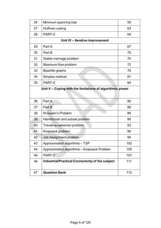
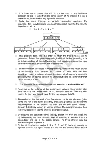
![Example: Knapsack of capacity W = 5
item weight value
1 2 $12
2 1 $10
3 3 $20
4 2 $15
0 1 2 3 4 5
0 0 0 0
w1 = 2, v1=
12
1 0 0 12
w2 = 1, v2=
10
2 0 10 12 22 22 2
2w3 = 3, v3=
20
3 0 10 12 22 30 3
2w4 = 2, v4=
15
4 15 25 30 0 10 3
7
Thus, the maximal value is V[4, 5] = $37.
Composition of an optimal subset:
The composition of an optimal subset can be found by tracing back the
computations of this entry in the table.
Since V[4, 5] ≠ V[3, 5], item 4 was included in an optimal solution along
with an optimal subset for filling 5 - 2 = 3 remaining units of the knapsack
capacity.
The latter is represented by element V[3, 3]. Since V[3, 3] = V[2, 3], item
3 is not a part of an optimal subset.
Since V[2, 3] ≠ V[l, 3], item 2 is a part of an optimal selection, which leaves
element
o V[l, 3 -1] to specify its remaining composition.
Similarly, since V[1, 2] ≠ V[O, 2], item 1 is the final part of the optimal solution
{item
o 1, item 2, item 4}.
Efficiency:
The time efficiency and space efficiency of this algorithm are both in
Θ(n W).
The time needed to find the composition of an optimal solution is in O(n
+ W).
Page 52 of 120](https://image.slidesharecdn.com/cs6402-scad-msm-191208081445/85/Cs6402-scad-msm-52-320.jpg)
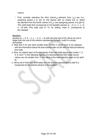
![3. Write an algorithm to construct an optimal binary search tree with
suitable example.
OPTIMAL BINARY SEARCH TREE Problem:
Given n keys a1 < …< an and probabilities p1,
…, pn searching for them, find a BST with a minimum average
number of comparisons in successful search.Since total number of BSTs with n
nodes is given by C(2n,n)/(n+1), which grows exponentially, brute force is
hopeless.
Let C[i,j] be minimum average number of comparisons made in T[i,j],
optimal BST for keys ai < …< aj , where 1 ≤ i ≤ j ≤ n. Consider optimal BST
among all BSTs with some ak (i ≤ k ≤ j ) as their root; T[i,j] is the best among them.
The recurrence for C[i,j]:
C[i,j] = min {C[i,k-1] + C[k+1,j]} + ∑ ps for 1 ≤ i ≤ j ≤ n
C[i,i] = pi for 1 ≤ i ≤ j ≤ n
C[i, i- 1] = 0 for 1≤ i ≤ n+1 which can be interpreted as the number of
comparisons in the empty tree.
0 1 j n
1 0 p 1 goal
0
p2
i C[i,j]
EXAMPLE
Page 53 of 120](https://image.slidesharecdn.com/cs6402-scad-msm-191208081445/85/Cs6402-scad-msm-53-320.jpg)
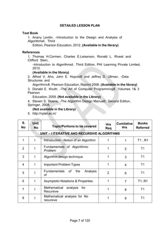
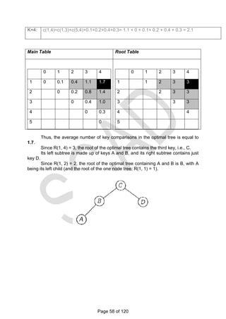
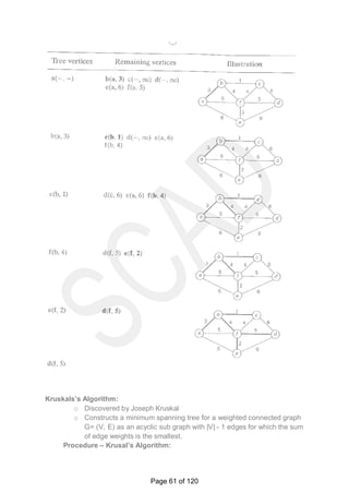
![Let us illustrate the algorithm by applying it to the four key set we used at the beginning of
this section:
KEY A B C D
PROBABILITY 0.1 0.2 0.4 0.3
Initial Tables:
Main Table Root Table
0 1 2 3 4
1 0 0.1
2 0 0.2
3 0 0.4
4 0 0.3
5 0
0 1 2 3 4
1 1
2 2
3 3
4 4
5
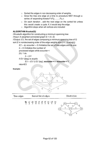
C(1,2): [i=1, j=2]
Possible key values k=1 and k=2.
K=1: c(1,2) = c(1,0) + c(2,2) + 0.1 + 0.2 = 0 + 0.2 + 0.1 + 0.2 = 0.5
K=2: c(1,2) = c(1,1) + c(3,2) + 0.1 + 0.2 = 0.1 + 0 + 0.1 + 0.2 = 0.4
Main Table Root Table
0 1 2 3 4
1 0 0.1 0.4
0 1 2 3 4
1 1 2
Page 54 of 120](https://image.slidesharecdn.com/cs6402-scad-msm-191208081445/85/Cs6402-scad-msm-54-320.jpg)
![2 0 0.2
3 0 0.4
4 0 0.3
5 0
2 2
3 3
4 4
5
C(2,3): [i=2, j=3]
Possible key values k=2 and k=3.
K=2: c(2,3) = c(2,1) + c(3,3) + 0.2 + 0.4 = 0 + 0.4 + 0.2 + 0.4 = 1.0
K=3: c(2,3) = c(2,2) + c(4,3) + 0.2 + 0.4 = 0.2 + 0 + 0.2 + 0.4 = 0.8
Main Table Root Table
0 1 2 3 4
1 0 0.1 0.4
2 0 0.2 0.8
3 0 0.4
4 0 0.3
5 0
0 1 2 3 4
1 1 2
2 2 3
3 3
4 4
5
C(3,4): [i=3, j=4]
Possible key values k=3 and k=4.
Page 55 of 120](https://image.slidesharecdn.com/cs6402-scad-msm-191208081445/85/Cs6402-scad-msm-55-320.jpg)
![K=3: c(3,4) = c(3,2) + c(4,4) + 0.4 + 0.3 = 0 + 0.3 + 0.4 + 0.3 = 1.0
K=4: c(3,4) = c(3,3) + c(5,4) + 0.4 + 0.3 = 0.4 + 0 + 0.4 + 0.3 = 1.1
Main Table Root Table
0 1 2 3 4
1 0 0.1 0.4
2 0 0.2 0.8
3 0 0.4 1.0
4 0 0.3
5 0
0 1 2 3 4
1 1 2
2 2 3
3 3 3
4 4
5
C(1,3): [i=1, j=3]
Possible key values k=1, k=2 and k=3.
K=1: c(1,3) = c(1,0) + c(2,3) + 0.1 + 0.2 + 0.4 = 0 + 0.8 + 0.1 + 0.2 + 0.4 = 1.5
K=2: c(1,3) = c(1,1) + c(3,3) + 0.1 + 0.2 + 0.4 = 0.1 + 0.4 + 0.1 + 0.2 + 0.4 = 1.2
K=3: c(1,3) = c(1,2) + c(4,3) + 0.1 + 0.2 + 0.4 = 0.4 + 0 + 0.1 + 0.2 + 0.4 = 1.1
Main Table Root Table
0 1 2 3 4
1 0 0.1 0.4 1.1
2 0 0.2 0.8
3 0 0.4 1.0
0 1 2 3 4
1 1 2 3
2 2 3
3 3 3
Page 56 of 120](https://image.slidesharecdn.com/cs6402-scad-msm-191208081445/85/Cs6402-scad-msm-56-320.jpg)
![4 0 0.3
5 0
4 4
5
C(2,4): [i=2, j=4]
Possible key values k=2, k=3 and k=4.
K=2: c(2,4) = c(2,1) + c(3,4) + 0.2 + 0.4 + 0.3 = 0 + 1.0 + 0.2 + 0.4 + 0.3 = 1.9
K=3: c(2,4) = c(2,2) + c(4,4) + 0.2 + 0.4 + 0.3 = 0.2 + 0.3 + 0.2 + 0.4 + 0.3 = 1.4
K=4: c(2,4) = c(2,3) + c(5,4) + 0.2 + 0.4 + 0.3 = 0.8 + 0 + 0.2 + 0.4 + 0.3 = 1.7
Main Table Root Table
0 1 2 3 4
1 0 0.1 0.4 1.1
2 0 0.2 0.8 1.4
3 0 0.4 1.0
4 0 0.3
5 0
0 1 2 3 4
1 1 2 3
2 2 3 3
3 3 3
4 4
5
C(1,4): [i=1, j=4]
Possible key values k=1, k=2, k=3 and k=4.
K=1: c(1,4)=c(1,0)+c(2,4)+0.1+0.2+0.4+0.3= 0 + 1.4 + 0.1+ 0.2 + 0.4 + 0.3 = 2.4
K=2: c(1,4)=c(1,1)+c(3,4)+0.1+0.2+0.4+0.3= 0.1 + 1.0 + 0.1+ 0.2 + 0.4 + 0.3 = 2.1
K=3: c(1,4)=c(1,2)+c(4,4)+0.1+0.2+0.4+0.3= 0.4 + 0.3 + 0.1+ 0.2 + 0.4 + 0.3 = 1.7
Page 57 of 120](https://image.slidesharecdn.com/cs6402-scad-msm-191208081445/85/Cs6402-scad-msm-57-320.jpg)


![There is a 1-1 correspondence between extreme points of LP‗s feasible
region and its basic feasible solutions.
Outline of Simplex Method:
Step 0 [Initialization] Present a given LP problem in standard
form and set up initial tableau.
Step 1 [Optimality test] If all entries in the objective row are nonnegative -
stop: the tableau
represents an optimal solution.
Step 2 [Find entering variable] Select (the most) negative
entry in the objective row. Mark its column to indicate the entering
variable and the pivot column.
Step 3 [Find departing variable] For each positive entry in the
pivot column, calculate the θ-ratio by dividing that row's entry in the
rightmost column by its entry in the pivot column. (If there are no positive
entries in the pivot column — stop: the problem is unbounded.) Find the
row with the smallest θ-ratio, mark this row to indicate the departing
variable and the pivot row.
Step 4 [Form the next tableau] Divide all the entries in the pivot row by its
entry in the pivot column. Subtract from each of the other rows, including
the objective row, the new pivot row multiplied by the entry in the pivot
column of the row in question. Replace the label of the pivot row by the
variable's name of the pivot column and go back to Step 1.
Page 83 of 120](https://image.slidesharecdn.com/cs6402-scad-msm-191208081445/85/Cs6402-scad-msm-83-320.jpg)


![for j := 1 to k-1 do
if(x[j]=I) or(abs(x[j]-I)=abs(j-k))) then return false;
return true;
}
Algorithm Nqueens(k,n)
{
for I:= 1 to n do
{
if( place(k,I) then
{
x[k]:= I;
if(k=n) then write(x[1:n]);
else
Nqueens(k
+1,n)
}
}
}
Example
N=4
2. Discuss in detail about Hamiltonian circuit problem and sum of subset
problem. (May/June
2016) (Nov/Dec 15)
Page 89 of 120](https://image.slidesharecdn.com/cs6402-scad-msm-191208081445/85/Cs6402-scad-msm-89-320.jpg)
![HAMILTONIAN CIRCUIT PROBLEM AND SUM OF SUBSET PROBLEM
A Hamiltonian circuit or Hamiltonian cycle is defined as a cycle that
passes through all the vertices of the graph exactly once. It is named after
the Irish mathematician Sir William Rowan Hamilton (1805-1865), who
became interested in such cycles as an application of his algebraic
discoveries. A Hamiltonian circuit can be also defined as a sequence of n
+ 1 adjacent vertices vi0,vi1…….vin,vi0 where the first vertex of the
sequence is the same as the last one while all the other n - 1 vertices are
distinct
Algorithm:(Finding all Hamiltonian cycle)
void Nextvalue(int k)
{
do
{
x[k]=(x[k]+1)%(n+1);
if(!x[k]) return; if(G[x[k-
1]][x[k]])
{
for(int j=1;j<=k-1;j++)
if(x[j]==x[k])
break;
}
}while(1);
}
if(j==k)
if(k<n)
return;void Hamiltonian(int k)
{
do
{
NextValue(k);
if(!x[k]) return;
if(k==n)
{
for(int i=1;i<=n;i++)
{
Print x[i];
}
}
else Hamiltonian(k+1);
}while(1);
}
Page 90 of 120](https://image.slidesharecdn.com/cs6402-scad-msm-191208081445/85/Cs6402-scad-msm-90-320.jpg)
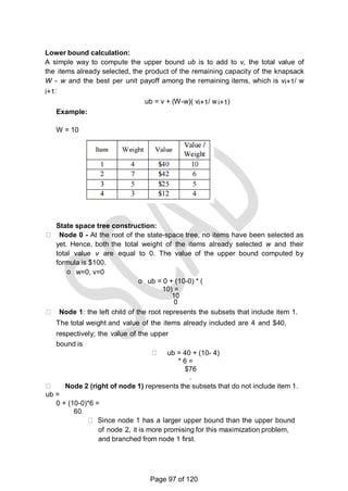
![//generate the left child. note s+w(k)<=M since
Bk-1 is true. X{k]=1;
if (S+W[k]=m) then write(X[1:k]); // there is no recursive call
here as
W[j]>0,1<=j<=n.
else if (S+W[k]+W[k+1]<=m) then sum of sub (S+W[k], k+1,r- W[k]);
//generate right child and evaluate Bk.
if ((S+ r- W[k]>=m)and(S+ W[k+1]<=m)) then
{
X{k]=0;
sum of sub (S, k+1, r- W[k]);
}
}
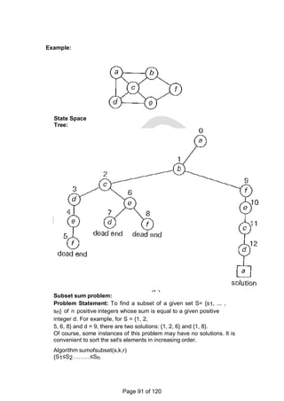
Construction of state space tree for subset sum:
The state-space tree can be constructed
as a binary tree.
The root of the tree represents the starting point, with no
decisions about the given elements made as yet.
Its left and right children represent, respectively, inclusion and
exclusion of s1 in a set being sought.
Similarly, going to the left from a node of the first level corresponds
to inclusion of s2, while going to the right corresponds to its
exclusion, and so on. Thus, a path from the root to a node on the ith
level of the tree indicates which of the first I numbers have been
included in the subsets represented by that node.
Record the value of s', the sum of these numbers, in the node. If s'
is equal to d, then there is a solution for this problem.
The result can be both reported and stopped or, if all the
solutions need to be found, continue by backtracking to the node's
parent. If s' is not equal to d, then terminate the node as non
promising if either of the following two inequalities holds:
s' + si+1 > d (the sums' is too large)
< (the sum is too small)
Page 92 of 120](https://image.slidesharecdn.com/cs6402-scad-msm-191208081445/85/Cs6402-scad-msm-92-320.jpg)
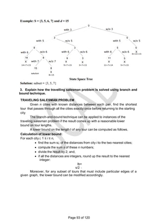
![graph.
For example, for the instance above the lower bound is:
lb = [(1+ 3) + (3 + 6) + (1 + 2) + (3 + 4) + (2 + 3)]/2 = 14.
The bounding function can be used, to find the shortest Hamiltonian circuit for
the given
Construction of state space tree:
Root:
First, without loss of generality, consider only tours that start at a.
First level
Second because the graph is undirected, tours can be generated in which b
is visited before c. In addition, after visiting n - 1 = 4 cities, a tour has no choice
but to visit the remaining unvisited city and return to the starting one.
Lower bound if edge (a,b) is chosen: lb =
ceil([(3+1)+(3+6)+(1+2)+(4+3)+(2+3)]/2)=14 Edge (a,c) is not include since b is
visited before c. Lower bound if edge (a,d) is chosen: lb =
ceil([5+1)+(3+6)+(1+2)+(5+3)+(2+3)]/2)=16. Lower bound if edge (a,e) is chosen: lb
= ceil([(8+1)+(3+6)+(1+2)+(4+3)+(2+8)]/2)=19 Since the lower bound of edge
(a,b) is smaller among all the edges, it is included in the solution. The state
space tree is expanded from this node.
Second level
The choice of edges should be made between three vertices: c, d and e.
Lower bound if edge (b,c) is chosen. The path taken will be (a ->b->c):
lb = ceil([(3+1)+(3+6)+(1+6)+(4+3)+(2+3)]/2)=16. Lower bound if edge (b,d) is
chosen. The path taken will be (a ->b->d):
lb = ceil([(3+1)+(3+7)+(7+3)+(1+2)+(2+3)]/2)=16
Page 94 of 120](https://image.slidesharecdn.com/cs6402-scad-msm-191208081445/85/Cs6402-scad-msm-94-320.jpg)
![Lower bound if edge (b,e) is chosen. The path taken will be (a ->b->e):
lb = ceil([(3+1)+(3+9)+(2+9)+(1+2)+(4+3)]/2)=19. (Since this lb is larger than other
values, so further expansion is stopped)
The path a->b->c and a->b->d are more promising. Hence the state space tree is
expanded from those nodes.
Next level
There are four possible routes:
a ->b->c->d->e->a a
->b->c->e->d->a a-
>b->d->c->e->a a-
>b->d->e->c->a
Lower bound for the route a ->b->c->d->e->a: (a,b,c,d)(e,a) lb =
ceil([(3+8)+(3+6)+(6+4)+(4+3)+(3+8)])
Lower bound for the route a ->b->c->e->d->a: (a,b,c,e)(d,a) lb =
ceil([(3+5)+(3+6)+(6+2)+(2+3)+(3+5)]/2)=19
Lower bound for the route a->b->d->c->e->a: (a,b,d,c)(e,a)
lb =
ceil([(3+8)+(3+7)+(7+4)+(4+2)+(2+8)]/2)
=24
Lower bound for the route a->b->d->e->c->a: (a,b,d,e)(c,a)
lb =
ceil([(3+1)+(3+7)+(7+3)+(3+2)+(2+1)]/2)
=16
Therefore from the above lower bound the solution is
The optimal tour is a ->b->c->e->d->a
The better tour is a ->b->c->e->d->a
The inferior tour is a->b->d->c->e->a
The first tour is a ->b->c->d->e->a
Page 95 of 120](https://image.slidesharecdn.com/cs6402-scad-msm-191208081445/85/Cs6402-scad-msm-95-320.jpg)
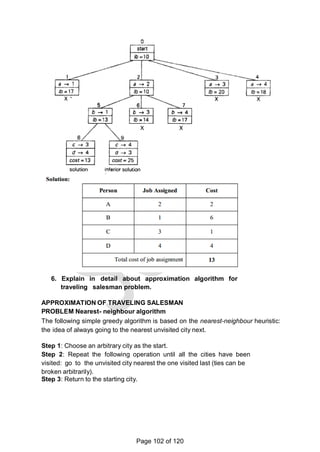
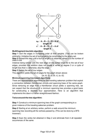
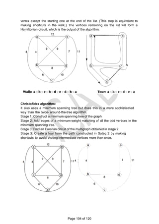
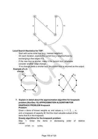
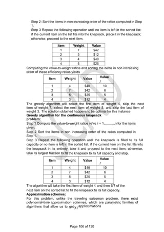


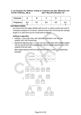
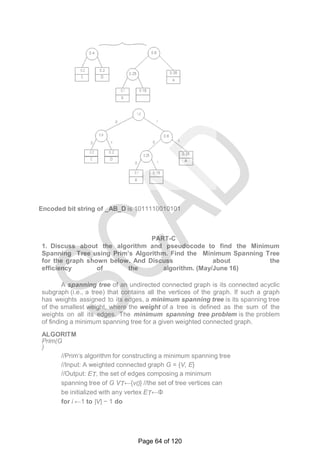
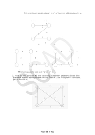
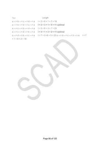
This document contains a syllabus for the subject "Design and Analysis of Algorithms". It discusses the following key points: - The objectives of the course are to learn algorithm analysis techniques, become familiar with different algorithm design techniques, and understand the limitations of algorithm power. - The syllabus is divided into 5 units which cover topics like introduction to algorithms, brute force and divide-and-conquer techniques, dynamic programming and greedy algorithms, iterative improvement methods, and coping with limitations of algorithmic power. - Examples of algorithms discussed include merge sort, quicksort, binary search, matrix multiplication, knapsack problem, shortest paths, minimum spanning trees, and NP-complete problems. - References