Operations Research

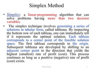
1. • Simplex: a linear-programming algorithm that can
solve problems having more than two decision
variables.
• The simplex technique involves generating a series of
solutions in tabular form, called tableaus. By inspecting
the bottom row of each tableau, one can immediately tell
if it represents the optimal solution. Each tableau
corresponds to a corner point of the feasible solution
space. The first tableau corresponds to the origin.
Subsequent tableaus are developed by shifting to an
adjacent corner point in the direction that yields the
highest (smallest) rate of profit (cost). This process
continues as long as a positive (negative) rate of profit
(cost) exists.
Simplex Method
Shiwani Gupta 1

2. Simplex algorithm
Initialization: setup to start iterations, including
finding an initial CPF solution
Optimality test: is the current CPF solution
optimal?
if no if yes stop
Iteration: Perform an iteration to find a
better CPF solutionShiwani Gupta 2

3. The simplex method in tabular form
Steps:
1. Initialization:
a. transform all the constraints to equality by
introducing slack, surplus, and artificial variables as
follows:
Constraint type Variable to be added
≤ + slack (s)
≥ - Surplus (s) + artificial (A)
= + Artificial (A)

4. Simplex method in tabular form
b. Construct the initial simplex tableau
Basic
variable
X1 … Xn S1 …Sn A1…. An RHS
S
Coefficient of the constraints
b1
A bm
Z Objective function coefficient
in different signs
Z value

5. 2. Test for optimality:
Case 1: Maximization problem
the current BF solution is optimal if every
coefficient in the objective function row is
nonnegative
Case 2: Minimization problem
the current BF solution is optimal if every
coefficient in the objective function row is
nonpositive
Simplex method in tabular form
Shiwani Gupta 5

6. Simplex method in tabular form
3. Iteration
Step 1: determine the entering basic variable by selecting
the variable (automatically a nonbasic variable) with
the most negative value (in case of maximization) or
with the most positive (in case of minimization) in the
last row (Z-row). Put a box around the column below
this variable, and call it the “pivot column”
Shiwani Gupta 6

7. Simplex method in tabular form
Step 2: Determine the leaving basic variable by applying
the minimum ratio test as following:
1. Pick out each coefficient in the pivot column that is
strictly positive (>0)
2. Divide each of these coefficients into the right hand side
entry for the same row
3. Identify the row that has the smallest of these ratios
4. The basic variable for that row is the leaving variable, so
replace that variable by the entering variable in the basic
variable column of the next simplex tableau. Put a box
around this row and call it the “pivot row”
Shiwani Gupta 7

8. Simplex method in tabular form
Step 3: Solve for the new BF solution by using elementary
row operations (multiply or divide a row by a nonzero
constant; add or subtract a multiple of one row to another
row) to construct a new simplex tableau, and then return
to the optimality test. The specific elementary row
operations are:
1. Divide the pivot row by the “pivot number” (the number
in the intersection of the pivot row and pivot column)
2. For each other row that has a negative coefficient in the
pivot column, add to this row the product of the absolute
value of this coefficient and the new pivot row.
3. For each other row that has a positive coefficient in the
pivot column, subtract from this row the product of the
absolute value of this coefficient and the new pivot row.
Shiwani Gupta 8

9. Simplex method
• Example (All constraints are )
Solve the following problem using the simplex method
• Maximize
Z = 3X1+ 5X2
Subject to
X1  4
2 X2  12
3X1 +2X2  18
X1 , X2  0
Shiwani Gupta 9

10. Simplex method
• Solution
• Initialization
1. Standard form
Maximize Z,
Subject to
Z - 3X1- 5X2 = 0
X1 + S1 = 4
2 X2 + S2 = 12
3X1 +2X2 + S3 = 18
X1 , X2, S1, S2, S3  0
Sometimes it is called the
augmented form of the
problem because the
original form has been
augmented by some
supplementary variables
needed to apply the
simplex method
Shiwani Gupta 10

11. Definitions
A basic solution is an augmented corner point solution.
A basic solution has the following properties:
1. Each variable is designated as either a nonbasic variable or a
basic variable.
2. The number of basic variables equals the number of
functional constraints. Therefore, the number of nonbasic
variables equals the total number of variables minus the
number of functional constraints.
3. The nonbasic variables are set equal to zero.
4. The values of the basic variables are obtained as
simultaneous solution of the system of equations (functional
constraints in augmented form). The set of basic variables
are called “basis”
5. If the basic variables satisfy the nonnegativity constraints,
the basic solution is a Basic Feasible (BF) solution.
Shiwani Gupta 11

12. Initial tableau
2. Initial tableau
Basic
variable
X1 X2 S1 S2 S3 RHS
S1 1 0 1 0 0 4
S2 0 2 0 1 0 12
S3 3 2 0 0 1 18
Z -3 -5 0 0 0 0
Pivot column
Pivot row
Pivot
number
Entering
variable
Leaving
variable

13. Simplex tableau
Notes:
The basic feasible solution at the initial tableau is
(0, 0, 4, 12, 18) where:
X1 = 0, X2 = 0, S1 = 4, S2 = 12, S3 = 18, and Z = 0
Where S1, S2, and S3 are basic variables
X1 and X2 are nonbasic variables
The solution at the initial tableau is associated to
the origin point at which all the decision
variables are zero.
Shiwani Gupta 13

14. Optimality test
By investigating the last row of the initial
tableau, we find that there are some negative
numbers. Therefore, the current solution is not
optimal.
Shiwani Gupta 14

15. Iteration
Step 1: Determine the entering variable by
selecting the variable with the most negative in
the last row.
• From the initial tableau, in the last row (Z row),
the coefficient of X1 is -3 and the coefficient of X2
is -5; therefore, the most negative is -5.
consequently, X2 is the entering variable.
• X2 is surrounded by a box and it is called the
pivot column
Shiwani Gupta 15

16. Iteration
Step 2: Determining the leaving variable by using the
minimum ratio test as following:
Basic
variable
Entering
variable X2
(1)
RHS
(2)
Ratio
(2)(1)
S1 0 4 None
S2
Leaving
2 12 6
Smallest ratio
S3 2 18 9

17. Iteration
Step 3: solving for the new BF solution by using the
eliminatory row operations as following:
1. New pivot row = old pivot row  pivot number
Basic
variable
X1 X2 S1 S2 S3 RHS
S1
X2 0 1 0 1/2 0 6
S3
Z
Note that X2 becomes in the basic
variables list instead of S2

18. iteration2. For the other row apply this rule:
New row = old row – the coefficient of this row in the pivot column (new pivot row).
For S1
1 0 1 0 0 4
-
0 (0 1 0 1/2 0 6)
1 0 1 0 0 4
For S3
3 2 0 0 1 18
-
2 (0 1 0 1/2 0 6)
3 0 0 -1 1 6
For Z
-3 -5 0 0 0 0
-
-5(0 1 0 1/2 0 6)
-3 0 0 5/2 0 30
Substitute this
values in the table
Shiwani Gupta 18

19. Iteration
Basic
variable
X1 X2 S1 S2 S3 RHS
S1 1 0 1 0 0 4
X2 0 1 0 1/2 0 6
S3 3 0 0 -1 1 6
Z -3 0 0 5/2 0 30
The most negative
value; therefore, X1
is the entering
variable
The smallest ratio is
6/3 =2; therefore, S3 is
the leaving variable
This solution is not optimal, since there is a negative numbers in the last row

20. Iteration
• Apply the same rules we will obtain this solution:
Basic
variable
X1 X2 S1 S2 S3 RHS
S1 0 0 1 1/3 -1/3 2
X2 0 1 0 1/2 0 6
X1 1 0 0 -1/3 1/3 2
Z 0 0 0 3/2 1 36
This solution is optimal; since there is no negative solution in the last row: basic
variables are X1 = 2, X2 = 6 and S1 = 2; the nonbasic variables are S2 = S3 = 0
Z = 36

21. Special cases of linear programming
• Infeasible solution
• Multiple solution (infinitely many solution)
• Unbounded solution
• Degenerated solution
Shiwani Gupta 21

22. Notes on the Simplex tableau1. In any Simplex tableau, the intersection of any basic variable with itself is always
one and the rest of the column is zeroes.
2. In any simplex tableau, the objective function row (Z row) is always in terms of
the nonbasic variables. This means that under any basic variable (in any tableau)
there is a zero in the Z row. For the non basic there is no condition ( it can take
any value in this row).
3. If there is a zero under one or more nonbasic variables in the last tableau (optimal
solution tableau), then there is a multiple optimal solution.
4. When determining the leaving variable of any tableau, if there is no positive ratio
(all the entries in the pivot column are negative and zeroes), then the solution is
unbounded.
5. If there is a tie (more than one variables have the same most negative or positive)
in determining the entering variable, choose any variable to be the entering one.
6. If there is a tie in determining the leaving variable, choose any one to be the
leaving variable. In this case a zero will appear in RHS column; therefore, a
“cycle” will occur, this means that the value of the objective function will be the
same for several iterations.
7. A Solution that has a basic variable with zero value is called a “degenerate
solution”.
8. If there is no Artificial variables in the problem, there is no room for “infeasible
solution”. Shiwani Gupta 22