1. 1
15. Poisson Processes
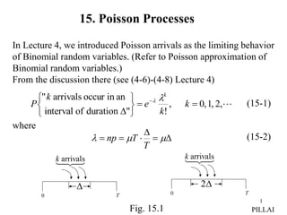
In Lecture 4, we introduced Poisson arrivals as the limiting behavior
of Binomial random variables. (Refer to Poisson approximation of
Binomial random variables.)
From the discussion there (see (4-6)-(4-8) Lecture 4)
where
,
2
,
1
,
0
,
!
"
duration
of
interval
an
in
occur
arrivals
"
k
k
e
k
P
k
(15-1)
T
T
np (15-2)
Fig. 15.1 PILLAI
0 T
arrivals
k
2
0 T
arrivals
k
2. 2
PILLAI
It follows that (refer to Fig. 15.1)
since in that case
From (15-1)-(15-4), Poisson arrivals over an interval form a Poisson
random variable whose parameter depends on the duration
of that interval. Moreover because of the Bernoulli nature of the
underlying basic random arrivals, events over nonoverlapping
intervals are independent. We shall use these two key observations
to define a Poisson process formally. (Refer to Example 9-5, Text)
Definition: X(t) = n(0, t) represents a Poisson process if
(i) the number of arrivals n(t1, t2) in an interval (t1, t2) of length
t = t2 – t1 is a Poisson random variable with parameter
Thus
(15-3)
.
2
2
2
1
T
T
np (15-4)
.
t
2
" arrivals occur in an (2 )
, 0, 1, 2, ,
interval of duration 2 " !
k
k
P e k
k
3. 3
PILLAI
and
(ii) If the intervals (t1, t2) and (t3, t4) are nonoverlapping, then the
random variables n(t1, t2) and n(t3, t4) are independent.
Since n(0, t) ~ we have
and
To determine the autocorrelation function let t2 > t1 ,
then from (ii) above n(0, t1) and n(t1, t2) are independent Poisson
random variables with parameters and respectively.
Thus
1
2
2
1 ,
,
2
,
1
,
0
,
!
)
(
}
)
,
(
{ t
t
t
k
k
t
e
k
t
t
n
P
k
t
(15-5)
),
,
( 2
1 t
t
RXX
),
( t
P
t
t
n
E
t
X
E
)]
,
0
(
[
)]
(
[ (15-6)
.
)]
,
0
(
[
)]
(
[ 2
2
2
2
t
t
t
n
E
t
X
E
(15-7)
1
t
)
( 1
2 t
t
).
(
)]
,
(
[
)]
,
0
(
[
)]
,
(
)
,
0
(
[ 1
2
1
2
2
1
1
2
1
1 t
t
t
t
t
n
E
t
n
E
t
t
n
t
n
E
(15-8)
4. 4
PILLAI
But
and hence the left side if (15-8) can be rewritten as
Using (15-7) in (15-9) together with (15-8), we obtain
Similarly
Thus
)
(
)
(
)
,
0
(
)
,
0
(
)
,
( 1
2
1
2
2
1 t
X
t
X
t
n
t
n
t
t
n
)].
(
[
)
,
(
)}]
(
)
(
){
(
[ 1
2
2
1
1
2
1 t
X
E
t
t
R
t
X
t
X
t
X
E XX
(15-9)
.
,
)]
(
[
)
(
)
,
(
1
2
2
1
2
1
1
2
1
2
1
2
2
1
t
t
t
t
t
t
X
E
t
t
t
t
t
RXX
(15-10)
(15-12)
(15-11)
.
,
)
,
( 1
2
2
1
2
2
2
1 t
t
t
t
t
t
t
RXX
).
,
min(
)
,
( 2
1
2
1
2
2
1 t
t
t
t
t
t
RXX
5. 5
PILLAI
From (15-12), notice that
the Poisson process X(t)
does not represent a wide
sense stationary process.
Define a binary level process
that represents a telegraph signal (Fig. 15.2). Notice that the
transition instants {ti} are random. (see Example 9-6, Text for
the mean and autocorrelation function of a telegraph signal).
Although X(t) does not represent a wide sense stationary process,
)
(
)
1
(
)
( t
X
t
Y
(15-13)
Fig. 15.2
0 1
t i
t
t
)
(t
X
t
)
(t
Y
t
1
Poisson
arrivals
1
1
t
6. 6
PILLAI
its derivative does represent a wide sense stationary process.
To see this, we can make use of Fig. 14.7 and (14-34)-(14-37).
From there
and
and
)
(t
X
)
(t
X )
(t
X
dt
d )
(
Fig. 15.3 (Derivative as a LTI system)
2
1 1 2
1 2
1 2 2
2 1 1 2
2
1 1 2
( , )
( )
( )
XX
XX
t t t
R t t
R t ,t
t t t t
t U t t
constant
a
dt
t
d
dt
t
d
t X
X
,
)
(
)
(
(15-14)
(15-15)
(15-16)
).
(
)
,
(
)
( 2
1
2
1
2
1
2
1 t
t
t
t
t
R
, t
t
R X
X
X
X
7. 7
PILLAI
From (15-14) and (15-16) it follows that is a wide sense
stationary process. Thus nonstationary inputs to linear systems can
lead to wide sense stationary outputs, an interesting observation.
• Sum of Poisson Processes:
If X1(t) and X2(t) represent two independent Poisson processes,
then their sum X1(t) + X2(t) is also a Poisson process with
parameter (Follows from (6-86), Text and the definition
of the Poisson process in (i) and (ii)).
• Random selection of Poisson Points:
Let represent random arrival points associated
with a Poisson process X(t) with parameter
and associated with
each arrival point,
define an independent
Bernoulli random
variable Ni, where
)
(t
X
.
)
( 2
1 t
,
,
,
, 2
1 i
t
t
t
,
t
.
1
)
0
(
,
)
1
( p
q
N
P
p
N
P i
i
(15-17)
1
t i
t
t
2
t
Fig. 15.4
8. 8
PILLAI
Define the processes
we claim that both Y(t) and Z(t) are independent Poisson processes
with parameters and respectively.
Proof:
But given X(t) = n, we have so that
and
Substituting (15-20)-(15-21) into (15-19) we get
pt
qt
k
n
n
t
X
P
n
t
X
k
t
Y
P
t
Y )}.
)
(
{
}
)
(
|
)
(
{
)
( (15-19)
)
(
)
(
)
1
(
)
(
;
)
(
)
(
1
)
(
1
t
Y
t
X
N
t
Z
N
t
Y
t
X
i
i
t
X
i
i
(15-18)
)
,
(
~
)
(
1
p
n
B
N
t
Y
n
i
i
{ ( ) | ( ) } , 0 ,
k n k
n
k
P Y t k X t n p q k n
(15-20)
( )
{ ( ) } .
!
n
t t
P X t n e
n
(15-21)
9. 9
PILLAI
More generally,
( ) ( )
!
( )! ! ! ( )!
(1 )
{ ( ) } ( )
!
( )
( ) , 0, 1, 2,
! !
~ ( ).
n n k
q t
k t
t q t
t k n k k
n
n k k n n k
n k n k
e
q t k
k pt
p e
P Y t k e p q t
k
e pt
pt e k
k k
P pt
(15-22)
( ( ) ) ( (
{ ( ) , ( ) } { ( ) , ( ) ( ) }
{ ( ) , ( ) }
{ ( ) | ( ) } { ( ) }
( ) ( ) ( )
( )! ! !
k m n n
k m t pt qt
k m
k
P Y t k P Z
P Y t k Z t m P Y t k X t Y t m
P Y t k X t k m
P Y t k X t k m P X t k m
t pt qt
p q e e e
k m k m
) )
{ ( ) } { ( ) },
t m
P Y t k P Z t m
(15-23)
10. 10
PILLAI
which completes the proof.
Notice that Y(t) and Z(t) are generated as a result of random Bernoulli
selections from the original Poisson process X(t) (Fig. 15.5),
where each arrival gets tossed
over to either Y(t) with
probability p or to Z(t) with
probability q. Each such
sub-arrival stream is also
a Poisson process. Thus
random selection of Poisson
points preserve the Poisson
nature of the resulting
processes. However, as we
shall see deterministic
selection from a Poisson
process destroys the Poisson
property for the resulting processes.
Fig. 15.5
t
t
q
p p p
)
(
~
)
( t
P
t
X
)
(
~
)
( qt
P
t
Z
t
q
p
)
(
~
)
( pt
P
t
Y
11. 11
PILLAI
Inter-arrival Distribution for Poisson Processes
Let denote the time interval (delay)
to the first arrival from any fixed point
t0. To determine the probability
distribution of the random variable
we argue as follows: Observe that
the event is the same as “n(t0, t0+t) = 0”, or the complement
event is the same as the event “n(t0, t0+t) > 0” .
Hence the distribution function of is given by
(use (15-5)), and hence its derivative gives the probability density
function for to be
i.e., is an exponential random variable with parameter
so that
1
,
1
"
" 1 t
1
1
( )
( ) , 0
t
dF t
f t e t
dt
(15-24)
(15-25)
1
.
/
1
)
( 1
E
Fig. 15.6
1
"
" 1 t
1
1
t n
t
t
2
t
1
Ist
2nd
arrival
nth
arrival
0
t
1 1 0 0
0 0
( ) { } { ( ) 0} { ( , ) 0}
1 { ( , ) 0} 1 t
F t P t P X t P n t t t
P n t t t e
12. 12
PILLAI
Similarly, let tn represent the nth random arrival point for a Poisson
process. Then
and hence
which represents a gamma density function. i.e., the waiting time to
the nth Poisson arrival instant has a gamma distribution.
Moreover
(15-26)
1
1 1
1 0
1
( ) ( ) ( )
( )
( 1)! !
, 0
( 1)!
n
n
k k
n n
t x x
t
k k
n n
x
dF x x x
f x e e
dx k k
x
e x
n
(15-27)
n
i
i
n
t
1
1
0
( ) { } { ( ) }
( )
1 { ( ) } 1
!
n
t n
k
n
t
k
F t P t t P X t n
t
P X t n e
k
13. 13
PILLAI
where is the random inter-arrival duration between the (i – 1)th
and ith events. Notice that are independent, identically distributed
random variables. Hence using their characteristic functions,
it follows that all inter-arrival durations of a Poisson process are
independent exponential random variables with common parameter
i.e.,
Alternatively, from (15-24)-(15-25), we have is an exponential
random variable. By repeating that argument after shifting t0 to the
new point t1 in Fig. 15.6, we conclude that is an exponential
random variable. Thus the sequence are independent
exponential random variables with common p.d.f as in (15-25).
Thus if we systematically tag every mth outcome of a Poisson process
X(t) with parameter to generate a new process e(t), then the
inter-arrival time between any two events of e(t) is a gamma
random variable.
i
.
( ) , 0.
i
t
f t e t
(15-28)
s
i
1
2
,
,
,
, 2
1 n
t
14. 14
Notice that
The inter-arrival time of e(t) in that case represents an Erlang-m
random variable, and e(t) an Erlang-m process (see (10-90), Text).
In summary, if Poisson arrivals are randomly redirected to form new
queues, then each such queue generates a new Poisson process
(Fig. 15.5). However if the arrivals are systematically redirected
(Ist arrival to Ist counter, 2nd arrival to 2nd counter, mth to mth ,
(m +1)st arrival to Ist counter, then the new subqueues form
Erlang-m processes.
Interestingly, we can also derive the key Poisson properties (15-5)
and (15-25) by starting from a simple axiomatic approach as shown
below:
),
,
.
/
1
)]
(
[
then
,
if
and
,
/
)]
(
[
t
e
E
m
m
t
e
E
PILLAI
15. 15
PILLAI
Axiomatic Development of Poisson Processes:
The defining properties of a Poisson process are that in any “small”
interval one event can occur with probability that is proportional
to Further, the probability that two or more events occur in that
interval is proportional to and events
over nonoverlapping intervals are independent of each other. This
gives rise to the following axioms.
Axioms:
(i)
(ii)
(iii)
and
(iv)
Notice that axiom (iii) specifies that the events occur singly, and axiom
(iv) specifies the randomness of the entire series. Axiom(ii) follows
from (i) and (iii) together with the axiom of total probability.
,
t
.
t
),
of
powers
(higher
),
( t
t
)
(
}
1
)
,
(
{ t
t
t
t
t
n
P
)
(
1
}
0
)
,
(
{ t
t
t
t
t
n
P
)
(
}
2
)
,
(
{ t
t
t
t
n
P
)
,
0
(
of
t
independen
is
)
,
( t
n
t
t
t
n
(15-29)
16. 16
PILLAI
We shall use these axiom to rederive (15-25) first:
Let t0 be any fixed point (see Fig. 15.6) and let represent the
time of the first arrival after t0 . Notice that the random variable
is independent of the occurrences prior to the instant t0 (Axiom (iv)).
With representing the distribution function of
as in (15-24) define Then for
From axiom (iv), the conditional probability in the above expression
is not affected by the event which refers to {n(t0, t0 + t) = 0},
i.e., to events before t0 + t, and hence the unconditional probability
in axiom (ii) can be used there. Thus
or
1
0
t
1
}
{
)
( 1
1
t
P
t
F
,
1
0
t
}
{ 1 t
1
1 0 0
1 0 0
0 0 1 1
( ) { }
{ , and no event occurs in ( , )}
{ , ( , ) 0}
{ ( , ) 0 | } { }.
Q t t P t t
P t t t t t t
P t n t t t t t
P n t t t t t t P t
)
(
)]
(
1
[
)
( t
Q
t
t
t
t
Q
0
( ) ( )
lim ( ) ( ) ( ) .
t
t
Q t t Q t
t Q t Q t Q t ce
1 1
( ) 1 ( ) { }.
Q t F t P t
17. 17
PILLAI
But so that
which gives
to be the p.d.f of as in (15-25).
Similarly (15-5) can be derived from axioms (i)-(iv) in (15-29) as well.
To see this, let
represent the probability that the total number of arrivals in the
interval (0, t) equals k. Then
1
}
0
{
)
0
( 1
P
Q
c
1
( ) 1 ( ) t
Q t F t e
1
( ) 1 , 0
t
F t e t
1
1
( )
( ) , 0
t
dF t
f t e t
dt
}
{
)}
)
,
0
(
{
)
( 3
2
1 X
X
X
P
k
t
t
n
P
t
t
pk
1
(15-30)
or
( ) { (0, ) )}, 0, 1, 2,
k
p t P n t k k
18. 18
PILLAI
where the events
are mutually exclusive. Thus
But as before
and
).
(
)
(
)
(
)
( 3
2
1 X
P
X
P
X
P
t
t
pk
t
p
t
k
t
n
P
k
t
n
t
t
t
n
P
X
P
t
p
t
k
t
n
P
t
t
t
n
P
k
t
n
P
k
t
n
t
t
t
n
P
X
P
k
k
1
2
1
}
1
)
,
0
(
{
}
1
)
,
0
(
|
1
)
,
(
{
)
(
)
(
)
1
(
}
)
,
0
(
{
}
0
)
,
(
{
}
)
,
0
(
{
}
)
,
0
(
|
0
)
,
(
{
)
(
0
)
( 3
X
P
1
2
3
= " (0, ) , and ( , ) 0"
= " (0, ) 1, and ( , ) 1"
= " (0, ) , and ( , ) 2"
X n t k n t t t
X n t k n t t t
X n t k i n t t t i
19. 19
where once again we have made use of axioms (i)-(iv) in (15-29).
This gives
or with
we get the differential equation
whose solution gives (15-5). Here [Solution to the above
differential equation is worked out in (16-36)-(16-41), Text].
This is completes the axiomatic development for Poisson processes.
PILLAI
.
0
)
(
1
t
p
)
(
)
(
)
1
(
)
( 1 t
tp
t
p
t
t
t
p k
k
k
)
(
)
(
)
(
lim
0
t
p
t
t
p
t
t
p
k
k
k
t
,
2
,
1
,
0
),
(
)
(
)
( 1
k
t
p
t
p
t
p k
k
k
20. 20
PILLAI
Poisson Departures between Exponential Inter-arrivals
Let and represent two independent
Poisson processes called arrival and departure processes.
)
(
~
)
( t
P
t
X )
(
~
)
( t
P
t
Y
Let Z represent the random interval between any two successive
arrivals of X(t). From (15-28), Z has an exponential distribution with
parameter Let N represent the number of “departures” of Y(t)
between any two successive arrivals of X(t). Then from the Poisson
nature of the departures we have
Thus
.
( )
{ | } .
!
k
t t
P N k Z t e
k
Fig. 15.7
1
t i
t
t
2
t 1
i
t
i
k
1
2
3
Z
)
(t
X
)
(t
Y
21. 21
PILLAI
i.e., the random variable N has a geometric distribution. Thus if
customers come in and get out according to two independent
Poisson processes at a counter, then the number of arrivals between
any two departures has a geometric distribution. Similarly the
number of departures between any two arrivals also represents
another geometric distribution.
(15-31)
0
( )
!
0
( )
0
0
!
!
1
!
{ } { | } ( )
( )
Z
k
t
t t
k
k t
k
k x
k
k
k
P N k P N k Z t f t dt
e e dt
t e dt
x e dx
, 0, 1, 2,
k
k
22. 22
PILLAI
Stopping Times, Coupon Collecting, and Birthday Problems
Suppose a cereal manufacturer inserts a sample of one type
of coupon randomly into each cereal box. Suppose there are n such
distinct types of coupons. One interesting question is that how many
boxes of cereal should one buy on the average in order to collect
at least one coupon of each kind?
We shall reformulate the above problem in terms of Poisson
processes. Let represent n independent
identically distributed Poisson processes with common parameter
Let represent the first, second, random arrival instants
of the process They will correspond to the first,
second, appearance of the ith type coupon in the above problem.
Let
so that the sum X(t) is also a Poisson process with parameter
)
(
,
),
(
),
( 2
1 t
X
t
X
t
X n
.
t
.
,
2,
1,
),
( n
i
t
Xi
,
, 2
1 i
i t
t
(15-32)
.
n
(15-33)
where
,
t
1
( ) ( ),
n
i
i
X t X t
23. 23
PILLAI
From Fig. 15.8, represents
The average inter-arrival duration
between any two arrivals of
whereas
represents the average inter-arrival
time for the combined sum process
X(t) in (15-32).
,
,
2,
1,
),
( n
i
t
Xi
/
1
/
1
Fig. 15.8
1
k
t 11
t
t
21
t 1
i
t
k
Y
1
Y 2
Y 3
Y
1
12
t 31
t
1
n
t
Nth
arrival
Ist
stopping
time T
Define the stopping time T to be that random time instant by which
at least one arrival of has occurred.
Clearly, we have
But from (15-25), are independent exponential
random variables with common parameter This gives
)
(
,
),
(
),
( 2
1 t
X
t
X
t
X n
n
i
ti ,
2,
1,
,
1
.
).
,
,
,
,
,
(
max 1
1
21
11 n
i t
t
t
t
T
(15-34)
.
)]
(
[
}
{
}
{
}
{
}
,
,
,
{
}
)
,
,
,
(
{max
}
{
)
(
1
21
11
1
21
11
1
21
11
n
ti
n
n
n
t
F
t
t
P
t
t
P
t
t
P
t
t
t
t
t
t
P
t
t
t
t
P
t
T
P
t
FT
24. 24
PILLAI
Thus
represents the probability distribution function of the stopping time
random variable T in (15-34). To compute its mean, we can make
use of Eqs. (5-52)-(5-53) Text, that is valid for nonnegative random
variables. From (15-35) we get
so that
Let so that
and
( ) (1 ) , 0
T
t n
F t e t
(15-35)
( ) 1 ( ) 1 (1 ) , 0
t n
T
P T t F t e t
(15-36)
0 0
{ } ( ) {1 (1 ) } .
t n
E T P T t dt e dt
1 ,
t
e x
,
(1 )
, or
t dx
x
e dt dx dt
n
k
k
n
n
k
x
dx
x
x
x
dx
x
dx
x
T
E
x
xn
1
1
0
1
0
1
2
1
0
1
0
1
1
1
1
1
1
)
1
(
1
)
1
(
}
{
25. 25
PILLAI
where is the Euler’s constant1.
Let the random variable N denote the total number of all arrivals
up to the stopping time T, and the inter-arrival
random variables associated with the sum process X(t) (see Fig 15.8).
1 Euler’s constant: The series converges, since
and so that Thus the series {un} converges
to some number From (1) we obtain also so that
1 1 1 1 1 1 1
{ } 1 1
2 3 2 3
1
(ln )
n
E T
n n
n n
0.5772157
(15-37)
N
k
Yk ,
2,
1,
,
3
1 1 1
{1 ln }
2 n n
2 2 2
1 1
1
0 0
1
x
n n n
dx dx
n
u
2
2
1
1 1
.
6
n
n
n n
u
0.
1
1
1
3
1 1 1
lim{1 ln } lim ln 0.5772157 .
2
n n
k k
n k
k
n n
u u
n n
(1)
1
1 1
( 1)
ln
n n
k k
k k
u n
1 1
1 1
( )
0 0
1
( )
1
ln 0
x
n n x n n x
n
dx dx n
n
u n
26. 26
Then we obtain the key relation
so that
since {Yi} and N are independent random variables, and hence
But so that and substituting this
into (15-37), we obtain
Thus on the average a customer should buy about or slightly
more, boxes to guarantee that at least one coupon of each
}
{
}
{
}]
|
{
[
}
{ i
Y
E
N
E
n
N
T
E
E
T
E
(15-40)
),
l(
Exponentia
~
i
Y
/
1
}
{
i
Y
E
{ } (ln ).
E N n n
(15-41)
,
lnn
n
N
i
i
Y
T
1
(15-38)
}
{
}
{
}
|
{
}
|
{
1
1
i
n
i
i
n
i
i Y
nE
Y
E
n
N
Y
E
n
N
T
E
(15-39)
27. 27
PILLAI
type has been collected.
Next, consider a slight generalization to the above problem: What if
two kinds of coupons (each of n type) are mixed up, and the objective
is to collect one complete set of coupons of either kind?
Let Xi(t) and Yi(t), represent the two kinds of
coupons (independent Poisson processes) that have been mixed up to
form a single Poisson process Z(t) with normalized parameter unity.
i.e.,
As before let represent the first, second, arrivals of
the process Xi(t), and represent the first, second,
arrivals of the process
n
i ,
2,
,
1
.
)
(
~
)]
(
)
(
[
)
(
1
n
i
i
i t
P
t
Y
t
X
t
Z (15-42)
,
, 2
1 i
i t
t
,
, 2
1 i
i
.
,
2,
1,
),
( n
i
t
Yi
28. 28
PILLAI
The stopping time T1 in this case represents that random instant at
which either all X – type or all Y – type have occurred at least
once. Thus
where
and
Notice that the random variables X and Y have the same distribution
as in (15-35) with replaced by 1/2n (since and there are 2n
independent and identical processes in (15-42)), and hence
Using (15-43), we get
}
,
min{
1 Y
X
T (15-43)
(15-44)
(15-45)
1
/2
( ) ( ) (1 ) , 0.
X Y
t n n
F t F t e t
(15-46)
11 21 1
max ( , , , )
n
X t t t
11 21 1
max ( , , , ).
n
Y
29. 29
PILLAI
to be the probability distribution function of the new stopping time T1.
Also as in (15-36)
1 1
/ 2 2
( ) ( ) (min{ , } )
1 (min{ , } ) 1 ( , )
1 ( ) ( )
1 (1 ( ))(1 ( ))
1 {1 (1 ) } , 0
T
X Y
t n n
F t P T t P X Y t
P X Y t P X t Y t
P X t P Y t
F t F t
e t
(15-47)
1
1 1
0 0
/ 2 2
0
{ } ( ) {1 ( )}
{1 (1 ) } .
T
t n n
E T P T t dt F t dt
e dt
/ 2 / 2 2
1 .
2 1
Let 1 , or ,
t n t n ndx
n x
e x e dt dx dt
1
0
1
2
1
0
1
0
2
1
)
1
)(
1
(
2
)
1
(
2
1
)
1
(
2
}
{
1
1
dx
x
x
x
x
n
dx
x
n
x
dx
x
n
T
E
n
n
n
n
n
x
x
30. 30
PILLAI
Once again the total number of random arrivals N up to T1 is related
as in (15-38) where Yi ~ Exponential (1), and hence using (15-40) we
get the average number of total arrivals up to the stopping time to be
We can generalize the stopping times in yet another way:
Poisson Quotas
Let
where Xi(t) are independent, identically distributed Poisson
1 1
1
1 0
0 0
1 1 1 1 1 1
1
2 3 1 2 2
{ } 2 ( )
2
2 (ln( / 2) ).
n n
k n k
k k
n n n n
E T n x x dx
n
n n
(15-48)
(15-49)
1
{ } { } 2 (ln( /2) ).
E N E T n n
)
(
~
)
(
)
(
1
t
P
t
X
t
X
n
i
i
(15-50)
31. 31
PILLAI
processes with common parameter so that
Suppose integers represent the preassigned number of
arrivals (quotas) required for processes in
the sense that when mi arrivals of the process Xi(t) have occurred,
the process Xi(t) satisfies its “quota” requirement.
The stopping time T in this case is that random time
instant at which any r processes have met their quota requirement
where is given. The problem is to determine the probability
density function of the stopping time random variable T, and
determine the mean and variance of the total number of random
arrivals N up to the stopping time T.
Solution: As before let represent the first, second,
arrivals of the ith process Xi(t), and define
Notice that the inter-arrival times Yij and independent, exponential
random variables with parameter and hence
t
i
.
2
1 n
n
m
m
m ,
,
, 2
1
)
(
,
),
(
),
( 2
1 t
X
t
X
t
X n
,
, 2
1 i
i t
t
1
,
j
i
ij
ij t
t
Y (15-51)
,
i
i
i
m
j
i
i
ij
m
i m
Y
t
1
, )
,
Gamma(
~
n
r
32. 32
PILLAI
Define Ti to the stopping time for the ith process; i.e., the occurrence
of the mi
th arrival equals Ti . Thus
or
Since the n processes in (15-49) are independent, the associated
stopping times defined in (15-53) are also
independent random variables, a key observation.
Given independent gamma random variables
in (15-52)-(15-53) we form their order statistics: This gives
Note that the two extremes in (15-54) represent
and
n
i
m
t
T i
i
m
i
i i
,
2,
1,
),
,
Gamma(
~
,
(15-52)
.
0
,
)!
1
(
)
(
1
t
m
t
t
f t
m
i
i
m
i
i
i
i
T
e
(15-53)
n
i
Ti ,
,
2
,
1
,
,
,
,
, 2
1 n
T
T
T
.
)
(
)
(
)
2
(
)
1
( n
r T
T
T
T
(15-54)
(15-55)
).
,
,
,
(
max
)
,
,
,
(
min
2
1
)
(
2
1
)
1
(
n
n
n
T
T
T
T
T
T
T
T
(15-56)
33. 33
PILLAI
The desired stopping time T when r processes have satisfied their
quota requirement is given by the rth order statistics T(r). Thus
where T(r) is as in (15-54). We can use (7-14), Text to compute the
probability density function of T. From there, the probability density
function of the stopping time random variable T in (15-57) is given by
where is the distribution of the i.i.d random variables Ti and
their density function given in (15-53). Integrating (15-53) by
parts as in (4-37)-(4-38), Text, we obtain
Together with (15-53) and (15-59), Eq. (15-58) completely specifies
the density function of the stopping time random variable T,
)
(t
F i
T
)
(t
f i
T
)
(r
T
T (15-57)
)
(
)]
(
1
)[
(
)!
(
)!
1
(
!
)
( 1
t
f
t
F
t
F
r
n
r
n
t
f i
T
i
T
i
T
T
k
n
k
(15-58)
.
0
,
!
)
(
1
)
(
1
0
t
e
k
t
t
F t
m
k
k
i i
i
i
T
(15-59)
34. 34
PILLAI
where r types of arrival quota requirements have been satisfied.
If N represents the total number of all random arrivals up to T,
then arguing as in (15-38)-(15-40) we get
where Yi are the inter-arrival intervals for the process X(t), and hence
with normalized mean value for the sum process X(t), we get
To relate the higher order moments of N and T we can use their
characteristic functions. From (15-60)
N
i
i
Y
T
1
(15-60)
}
{
}
{
}
{
}
{ 1 N
E
Y
E
N
E
T
E i
(15-61)
(15-62)
)
1
(
}.
{
}
{ T
E
N
E
1 1
[ { }]
{ } { } { [ | ]}
[{ { }| } ].
N n
i i
i i
j Y n
i
i
j Y j Y
j T
E e
j Y n
E e E e E E e N n
E E e N n
(15-63)
35. 35
PILLAI
But Yi ~ Exponential (1) and independent of N so that
and hence from (15-63)
which gives (expanding both sides)
or
a key identity. From (15-62) and (15-64), we get
1
{ | } { }
1
i i
j Y j Y
E e N n E e
j
0
1
1
{ } [ { }] ( ) {(1 ) }
i
N
j Y
j T n N
n
j
E e E e P N n E E j
0
0
)}
1
(
)
1
(
{
}
{ !
)
(
!
)
(
k
k
k
k
k
k
N
N
N
E
T
E k
j
k
j
)},
1
(
)
1
(
{
}
{
k
N
N
N
E
T
E k
}.
{
}
{
var
}
{
var T
E
T
N
(15-64)
(15-65)
36. 36
PILLAI
As an application of the Poisson quota problem, we can reexamine
the birthday pairing problem discussed in Example 2-20, Text.
“Birthday Pairing” as Poisson Processes:
In the birthday pairing case (refer to Example 2-20, Text), we
may assume that n = 365 possible birthdays in an year correspond to
n independent identically distributed Poisson processes each with
parameter 1/n, and in that context each individual is an “arrival”
corresponding to his/her particular “birth-day process”. It follows that
the birthday pairing problem (i.e., two people have the same birth date)
corresponds to the first occurrence of the 2nd return for any one of
the 365 processes. Hence
so that from (15-52), for each process
Since and from (15-57) and (15-66) the stopping time
in this case satisfies
1
,
2
2
1
r
m
m
m n
(15-66)
).
1/
(2,
Gamma
~ n
Ti
,
/
1
/ n
n
i
(15-67)
).
,
,
,
(
min 2
1 n
T
T
T
T
(15-68)
37. 37
PILLAI
Thus the distribution function for the “birthday pairing” stopping
time turns out to be
where we have made use of (15-59) with
As before let N represent the number of random arrivals up to the
stopping time T. Notice that in this case N represents the number of
people required in a crowd for at least two people to have the same
birth date. Since T and N are related as in (15-60), using (15-62) we get
To obtain an approximate value for the above integral, we can expand
in Taylor series. This gives
.
/
1
and
2 n
m i
i
1 2
( ) { } 1 { }
1 {min ( , , , ) }
1 [ { }] 1 [1 ( )]
1 (1 )
T
Ti
n
n n
i
n t
t
n
F t P T t P T t
P T T T t
P T t F t
e
(15-69)
)
1
ln(
)
1
ln( n
t
n
t n
n
0
0 0
{ } { } ( )
{1 ( )} (1 ) .
T
n t
t
n
E N E T P T t dt
F t dt e dt
(15-70)
38. 38
PILLAI
and hence
so that
and substituting (15-71) into (15-70) we get the mean number of
people in a crowd for a two-person birthday coincidence to be
On comparing (15-72) with the mean value obtained in Lecture 6
(Eq. (6-60)) using entirely different arguments
2 3
2 3
1
ln
2 3
t
n
t t t
n n n
2 3
2 2
3
( )
1
t t
n n
t
n
t
n
e
3
2 2
2
2 3 2
3
2
1 1
3
t
t t
n n n
t
n t
t
n n
e e e e
(15-71)
2 2
2
2
2
/ 2 3 / 2
0 0
0
1
3
2
1
2
2 3
{ }
2
2
3
24.612.
t n t n
x
n
n n
n
E N e dt t e dt
n xe dx
(15-72)
( { } 24.44),
E X
39. 39
we observe that the two results are essentially equal. Notice that the
probability that there will be a coincidence among 24-25 people is
about 0.55. To compute the variance of T and N we can make use of
the expression (see (15-64))
which gives (use (15-65))
The high value for the standard deviations indicate that in reality the
crowd size could vary considerably around the mean value.
Unlike Example 2-20 in Text, the method developed here
can be used to derive the distribution and average value for
2 2
2
0
/ 2 4 / 2
2
0 0 0
2
2
0
2
1
3
3
2
8
3
{ ( 1)} { } 2 ( )
2 2
2 (2 ) 2 2 2
t t n t n
x
n
t
n n
n
E N N E T tP T t dt
t e dt t e dt t e dt
n e dx n n n n
(15-73)
.
146
.
12
,
12
.
13
N
T
(15-74)
PILLAI
40. 40
a variety of “birthday coincidence” problems.
Three person birthday-coincidence:
For example, if we are interested in the average crowd size where
three people have the same birthday, then arguing as above, we
obtain
so that
and T is as in (15-68), which gives
to be the distribution of the
stopping time in this case. As before, the average crowd size for three-
person birthday coincidence equals
,
1
,
3
2
1
r
m
m
m n
(15-75)
)
/
1
,
3
(
Gamma
~ n
Ti (15-76)
2
2
( ) 1 [1 ( )] 1 1 , 0
2
i
n
n t
T T
t t
F t F t e t
n n
2
2
0 0
{ } { } ( ) 1 .
2
n
t
t t
E N E T P T t dt e dt
n n
(15-77)
PILLAI
)
/
1
,
3
with
59)
-
(15
(use n
m i
i
41. 41
By Taylor series expansion
so that
Thus for a three people birthday coincidence the average crowd size
should be around 82 (which corresponds to 0.44 probability).
Notice that other generalizations such as “two distinct birthdays
to have a pair of coincidence in each case” (mi =2, r = 2) can be easily
worked in the same manner.
We conclude this discussion with the other extreme case,
where the crowd size needs to be determined so that “all days
in the year are birthdays” among the persons in a crowd.
3
3
3
2
2
2
2
2
2
2
2
2
6
2
3
1
2
2
1
2
2
1
ln
n
t
n
t
n
t
n
t
n
t
n
t
n
t
n
t
n
t
n
t
3 2 1/3 2/3
/6
0 0
1/3 2/3
1 1
3
6
3
{ }
6 (4/3) 82.85.
t n x
n
E N e dt x e dx
n
(15-78)
PILLAI
42. 42
All days are birthdays:
Once again from the above analysis in this case we have
so that the stopping time statistics T satisfies
where Ti are independent exponential random variables with common
parameter This situation is similar to the coupon collecting
problem discussed in (15-32)-(15-34) and from (15-35), the
distribution function of T in (15-80) is given by
and the mean value for T and N are given by (see (15-37)-(15-41))
Thus for “everyday to be a birthday” for someone in a crowd,
365
,
1
2
1
n
r
m
m
m n
(15-79)
),
,
,
,
(
max 2
1 n
T
T
T
T
(15-80)
.
1
n
/
( ) (1 ) , 0
T
t n n
F t e t
(15-81)
{ } { } (ln ) 2,364.14.
E N E T n n
(15-82)
PILLAI
43. 43
the average crowd size should be 2,364, in which case there is 0.57
probability that the event actually happens.
For a more detailed analysis of this problem using Markov chains,
refer to Examples 15-12 and 15-18, in chapter 15, Text. From there
(see Eq. (15-80), Text) to be quite certain (with 0.98 probability) that
all 365 days are birthdays, the crowd size should be around 3,500.
PILLAI
44. 44
Bulk Arrivals and Compound Poisson Processes
In an ordinary Poisson process X(t), only one event occurs at
any arrival instant (Fig 15.9a). Instead suppose a random number
of events Ci occur simultaneously as a cluster at every arrival instant
of a Poisson process (Fig 15.9b). If X(t) represents the total number of
all occurrences in the interval (0, t), then X(t) represents a compound
Poisson process, or a bulk arrival process. Inventory orders, arrivals
at an airport queue, tickets purchased for a show, etc. follow this
process (when things happen, they happen in a bulk, or a bunch of
items are involved.)
t
1
t 2
t n
t
t
1
t 2
t n
t
3
1
C
2
2
C
4
i
C
(a) Poisson Process (b) Compound Poisson Process
Let
,
2
,
1
,
0
},
{
k
k
C
P
p i
k
Fig. 15.9
(15-83)
PILLAI
45. 45
PILLAI
represent the common probability mass function for the occurrence
in any cluster Ci. Then the compound process X(t) satisfies
where N(t) represents an ordinary Poisson process with parameter Let
represent the moment generating function associated with the cluster
statistics in (15-83). Then the moment generating function of the
compound Poisson process X(t) in (15-84) is given by
( )
1
( ) ,
N t
i
i
X t C
(15-84)
0
}
{
)
(
k
k
k
C
z
p
z
E
z
P i
(15-85)
1
( )
0
( )
0
(1 ( ))
0
( )
!
( ) { ( ) } { }
{ [ | ( ) ]} [ { | ( ) }]
( { }) { ( ) }
( )
X
k
i
i
k
C
i
n X t
n
X t
C k
k
k t t P z
k
t
k
z z P X t n E z
E E z N t k E E z N t k
E z P N t k
P z e e
(15-86)
.
46. 46
PILLAI
If we let
where represents the k fold convolution of the sequence {pn}
with itself, we obtain
that follows by substituting (15-87) into (15-86). Eq. (15-88)
represents the probability that there are n arrivals in the interval (0, t)
for a compound Poisson process X(t).
Substituting (15-85) into (15-86) we can rewrite also as
where which shows that the compound Poisson process
can be expressed as the sum of integer-secaled independent
Poisson processes Thus
}
{ )
(k
n
p
( )
0
( )
!
{ ( ) }
k
t k
n
k
t
k
P X t n e p
(15-88)
(15-87)
)
(z
X
2
1 2 (1 )
(1 ) (1 )
( )
k
k
X
t z
t z t z
z e e e
(15-89)
,
k
k p
.
),
(
),
( 2
1
t
m
t
m
( )
0 0
( )
k
k k k n
n n
n n
P z p z p z
47. 47
PILLAI
More generally, every linear combination of independent Poisson
processes represents a compound Poisson process. (see Eqs. (10-120)-
(10-124), Text).
Here is an interesting problem involving compound Poisson processes
and coupon collecting: Suppose a cereal manufacturer inserts either
one or two coupons randomly – from a set consisting of n types of
coupons – into every cereal box. How many boxes should one buy
on the average to collect at least one coupon of each type? We leave
it to the reader to work out the details.
.
)
(
)
(
1
k
k t
m
k
t
X (15-90)