Based on the knowledge of dynamic systems, the shorter the transient response, or the faster a system reaches the steady-state after the introduction of the change, the smaller will be the output variability. In lean manufacturing, the principle of reducing set-up times has the same purpose: reduce the transient time and improve production flow. Analogously, the analysis of the transient response of project-driven systems may provide crucial information about how fast these systems react to a change and how that change affects their production output. Although some studies have investigated flow variability in projects, few have looked at variability from the perspective that the transient state represents the changeovers on project-driven production systems and how the transient state affects the process’ flow variability. The purpose of this study is to investigate the effect of changes in project-driven production systems from a conceptual point of view, furthermore, measuring and correlating the transient response of five cases to their flow variability. Results showed a proportional relationship between the percentile transient time and flow variability of a process. That means that the quicker the production system reacts to change; the less the distress in the production output, consequently, lower levels of flow variability. As practical implications, lean practices focusing on reducing set-up times (transient time) can have their effects measured on project-driven production flow.

1. Antunes, R., Gonzalez, V., and Walsh, K. 2016. “Quicker reaction, lower variability: The effect of transient
time in flow variability of project-driven production” Proc. 24rd
Ann. Conf. of the Int’l. Group for Lean
Construction, 21-23 July, Boston, MA, sect.1 pp. 73-82, available at www.iglc.net
73
Section 1: Theory
QUICKER REACTION, LOWER
VARIABILITY: THE EFFECT OF TRANSIENT
TIME IN FLOW VARIABILITY OF PROJECT-
DRIVEN PRODUCTION
Ricardo Antunes1, Vicente González2, and Kenneth Walsh3
ABSTRACT
Based on the knowledge of dynamic systems, the shorter the transient response, or the
faster a system reaches the steady-state after the introduction of the change, the smaller
will be the output variability. In lean manufacturing, the principle of reducing set-up
times has the same purpose: reduce the transient time and improve production flow.
Analogously, the analysis of the transient response of project-driven systems may provide
crucial information about how fast these systems react to a change and how that change
affects their production output. Although some studies have investigated flow variability
in projects, few have looked at variability from the perspective that the transient state
represents the changeovers on project-driven production systems and how the transient
state affects the process’ flow variability. The purpose of this study is to investigate the
effect of changes in project-driven production systems from a conceptual point of view,
furthermore, measuring and correlating the transient response of five cases to their flow
variability. Results showed a proportional relationship between the percentile transient
time and flow variability of a process. That means that the quicker the production system
reacts to change; the less the distress in the production output, consequently, lower levels
of flow variability. As practical implications, lean practices focusing on reducing set-up
times (transient time) can have their effects measured on project-driven production flow.
KEYWORDS
Flow, variability, production, Single Minute Exchange of Dies (SMED), productivity
function
1
Ph.D. candidate, Department of Civil and Environmental Engineering - University of
Auckland, New Zealand, rsan640@aucklanduni.ac.nz
2
Senior Lecturer, Department of Civil and Environmental Engineering - University of
Auckland, New Zealand, v.gonzalez@auckland.ac.nz
3
Dean, SDSU-Georgia, San Diego State University, Tbilisi, Georgia, kwalsh@mail.sdsu.edu

2. Ricardo Antunes, Vicente González, and Kenneth Walsh
74 Proceedings IGLC-24, July 2016 | Boston, USA
INTRODUCTION
The importance of the time spent in production changeovers has been well-known for a
long time (Taylor, 1911), as much as structured approaches to reduce such time (Gilbreth,
1911). However, it was later with the development of ‘Just-In-Time’ that progress was
made to lessen the changeover time. Observations of how to reduce the time spent on the
exchange of dies on automotive pressing machines resulted in a structured methodology
capable of bringing down the time spent in changeovers from hours to minutes (Shingō,
1985). Widely applied in the manufacturing till this day, the Single Minute Exchange of
Dies (SMED) consists of seven basic steps. The steps are:
(I) observe and measure the current methodology;
(II) separate external of internal activities;
(III) transform internal activities into external ones;
(IV) simplify remaining internal activities;
(V) make the external activities more efficient;
(VI) standardize the new procedure; and
(VII) repeat the method for further improvement
THE 3 UPS OF CHANGEOVER
A process changeover (Figure 1) consists of three ‘ups’:
Cleanup
Cleanup is the removal of previous product, materials, components, and/or residuals from
the production line or site. It may range from minor tasks such as cleaning after a
painting job has finished to major work such as a tower crane disassembling. ‘5S’
practices perform a significant role in the cleanup stage, simply because if there is less to
clean, it can be done faster (Womack, Jones, and Roos, 1991). Hence, keep a clean and
organized site supports a quicker cleaning. Ideally, the cleanup finishes with the
production output. It means that once a production output reaches zero, the site is clean.
Accordingly, the cleanup stage can be measurable. It starts when the input of the
production system ceases. In the best case scenario, the cleanup finishes when the process
output reaches zero, i.e., there is nothing else to be produced or cleaned. Otherwise, the
cleanup finishes when everything needed in the process is removed.
Setup
Setup is the group of activities of converting the site to run a new process. The
conversion requires adjusting or parametrizing equipment to match the requirements of
the next production process or by replacing non-adjustable equipment. Usually, it
involves a combination of both. For that reason, the resources are applied for preparing
the site for the process while the production process stands still waiting to start. This
situation is the muda of waiting (Ohno, 1988), or simply waste. The setup stage is utterly
unproductive; it adds no value. Therefore, lean practices aim to ‘zero setups’ or
‘eliminate setup’. The setup is also measurable. It begins when cleanup finishes and ends

3. Quicker Reaction, Lower Variability: The Effect of Transient Time in Flow Variability of Project-Driven
Production
Section 1: Theory 75
at the production kick-off.
Startup
Startup (transient) is the time immediately after a process kick-off until the full process
operation (steady-state). The initial moments involve ‘learning’ and fine-tuning the
equipment and the pace of work. In this stage, jams and stoppages are frequent causing
defective products and variations in the production output (Shingō, 1985). The
production system often underperforms at the setup stage in comparison to the production
at steady-state.
Figure 1 - Process changeover
SMED AND CONSTRUCTION
The main focus of SMED is the transformation of internal activities of the setup stage to
external activities. In manufacturing, an internal activity is any operation that can only be
performed if the machine is shut down (for instance, attaching or removing the dies). An
external activity can be executed when the machine is running (Cakmakci, 2008). In
project management terms, internal activities are in the critical path, while external
activities are parallel to the critical path. Hence, in a project-driven process, the
application of SMED means removing activities that are not hardwired to the critical path
and executing them in parallel, furthermore, resulting in a compressed critical path. In the
end, SMED practices in project management can be seen as a method for fast tracking the
project schedule.
The concept and benefits of SMED are well known in the construction industry,
especially within the lean construction community. An example of the use of SMED
Process changeovery(t)
t
Steady-state
● The system reaches an equilibrium
condition
● Minimal (natural) variations are
allowed
Startup (Transient)
● The system changes fast
● Different outputs levels
observed for a fixed input
(high flow variability)
ts (settling time)
threshold (natural variabilty)
Production
Loss
Setup
● No input into the system
● There is no production output
● External activities
Cleanup
● No input into
the system
● Output is due
work-in-progress
steady-state
t0 (kick off time)

4. Ricardo Antunes, Vicente González, and Kenneth Walsh
76 Proceedings IGLC-24, July 2016 | Boston, USA
practices in construction is the offsite fabrication (Gibb, 1999). On offsite fabrication
building tasks are performed externally to the site and what is left is a reduced number of
assembling activities to be performed onsite. Automation is another example of the use of
SMED, in particular, the application of techniques to eliminate adjustments and improve
mechanization. Construction processes are flexible, constituted by a workforce,
machinery and equipment with relatively general purpose (Hayes and Wheelwright,
1979, p. 134). Such flexibility favors the adaptation of existing resources to new
processes over resources replacement in the setup stage. However, there is still the
‘adjusting or parametrizing equipment’ to do. Automatic parametric machinery may
reduce the time of setup times by performing the conversion faster and improve startup
because it may reduce the possibility of human error while adjusting the machinery.
Although the use of offsite fabrication and automation in construction are strongly related
to SMED and widely present in the construction industry, little is the discussion about the
structured application of SMED as performed in manufacturing. Even though, the
implementation of SMED in construction is likely to be easier than in manufacturing
based on general purpose equipment and workforce in the construction industry.
As all continuous improvement techniques, SMED requires measurement, control,
comparison and benchmarking. As measurements, SMED usually utilizes the estimator of
Process Performance Index (assuming that the process output is approximately normally
distributed), Cpk, and Process Performance, Pp, values for judging a process, whether it is
capable of improvement or not (Cakmakci, 2008). Cpk is the result of the upper
specification limit minus the mean of the output divided by three times the output sample
standard deviation; or, the mean of the output minus the lower specification limit divided
by three times the output sample standard deviation. Whatever shows the minimum value
(Montgomery, 2009, p. 355). The Pp is given by the difference of upper specification
limit and lower specification limit (here plus and minus two percent around the mean,
matching the threshold limits) divided by six times the standard deviation of output
sample (Montgomery, 2009, p. 363).
Those formulas provide unique values of Cpk and Pp that can be used in the judgment,
what works fine for manufacturing. Construction is a different story. The difficulty in
judging a construction process is due to the short run (batch size) of its production
(Antunes and Gonzalez, 2015). In other words, there is not a long enough—sometimes
any—steady-state to produce useful data (normal distribution around the steady-state
value) to use Cpk and Pp. The highly variable and long transient state of project-driven
processes disrupt the accuracy of the values given by Cpk and Pp. Because they end up
accounting for variations in transient—and consequently setup—stages rather than the
variations at steady-state. Another difficulty is in defining what are the upper and lower
limits of variation once project management problems may have several suitable
solutions.
FLOW VARIABILITY
In a process chain (Figure 2), the output of a process is the input of another,
consequently, establishing a flow. When variations of the output of the process i affects
the input, and/or behavior of the following process, i+1, this is called flow variability.

5. Quicker Reaction, Lower Variability: The Effect of Transient Time in Flow Variability of Project-Driven
Production
Section 1: Theory 77
How much the output variation of the process i affects the process i+1, depends on two
factors. One is the coefficient of variation of the arrival rate of the process i+i, ca. In a
process chain, without yield less or rework, the arrival rate of the process i+1 is equal to
of the departure rate of the process i, as well as the coefficient of variations, cd(i) = ca(i+1).
That is known as the conservation of material (Hopp and Spearman, 2001, p. 253).
Figure 2: Propagation of variability between processes. Adapted from Factory Physics:
Foundations of Manufacturing Management, 2nd ed. (p. 262), by Hopp, W. J., and
Spearman, M. L., 2001, Irwin McGraw-Hill.
The second factor is the utilization, u, of the process i+1. u values close to one indicate a
process almost always busy, on the other hand, values close to zero points out a process
nearly always idle. Since u is likely to assume values between zero and one the output
variation of the process, cd(i+1), is given by Equation 1. Accordingly, if the output of the
upstream process i is highly variable, the output of the downstream process i+1 is also
highly variable (Hopp and Spearman, 2001, p. 261).
Equation 1: Coefficient of the departure of the downstream process
MEASURING PROCESS’ TRANSIENT
The direct method of measuring a process’ transient is to compute the amount of output
at regular intervals of time, e.g., ‘Time and Motion’ (Taylor, 1911). Nevertheless, to
calculate the transient time, ts, the process must reach the steady-state. Hence, the data
collection must proceed until the steady-state is reached and is undisputed that the
process is in this state. Such procedure seems impractical as a non-automated task.
Because, that means to utilize a workforce to monitor, measure and count the production
output regularly in short periods of time. Even, after all, it may be impossible obtaining
the process’ transient time because construction processes often do not reach the steady-
state.
PRODUCTIVITY FUNCTION METHOD
A productivity function, P(t), represents the relation between the output function, Y(t),
and the input function, U(t), of a project-driven production process, Y(t) = P(t)*U(t),
* symbolizes the convolution operator. Approaching the production process as a dynamic
system the productivity function accounts for the transient and steady/unsteady-state
(Antunes, González, and Walsh, 2015). The transient time is given by the transient
analysis (Figure 2) of a processes’ productivity function. The transient time, ts, is the time
ca(i) Process
i+1
Process
i
cd(i) = ca(i+1) cd(i+1)
ce(i) ce(i+1)
cd(i+1)
2
= u2
ce(i+1)
2
+(1 u2
)ca(1+i)
2

6. Ricardo Antunes, Vicente González, and Kenneth Walsh
78 Proceedings IGLC-24, July 2016 | Boston, USA
the output takes to reach the steady-state value, or a threshold around the steady-state
value (usually, –+2%) from the moment a unitary step input is applied, t0. The step input
acts as an off-on switch, e.g., a light switch, which the input changes instantaneously
from zero to one. The change in the input provokes the reaction of the system that tries to
adapt as fast as possible (the bulb light filament warms once there is an electric current).
Later on, the output tends to a constant value when t → ∞ (the filament reached a
temperature in which it produces a steady amount of light). The percentile reaction time
is obtained by dividing the process transient time, ts, by the total process time, tt.
Figure 2 - Transient analysis
Some studies have investigated flow variability in projects. However, few have
investigated the relation and effects of the transient state on flow variability of project-
driven production systems. This study aims to examine, from a conceptual standpoint, the
effect that changes in project-driven production systems have on their flow variability.
Furthermore, measure and correlate the transient response of five cases to their flow
variability.
METHOD
This research analyzed five cases with different sample sizes, and the processes compile
various activities in construction. The cases are:
Case 1: drilling an offshore oil well (Antunes et al., 2015),
Case 2: wall assembling (Abdel-Razek, Elshakour, and Abdel-Hamid, 2007),
Case 3: setting formwork for slabs,
Case 4: group of activities (foundation excavation and backfill) from a housing
project, and
Case 5: wall plastering (González, Alarcón, Maturana, Mundaca, and Bustamante,
2010).
The commonality among the cases is that they configure a system, i.e., they are
constituted by input, transformation process, and output.
First, the process output variation is measured. Process Performance Index, Cpk, and
Process Performance, Pp, are obtained for the cases and shown in Table 1. A third
measurement of output variation is given by the coefficient of variation (Hopp and
Spearman, 2001, p. 252) of the departure times the process i, cd(i). That is the result of the
ratio of standard deviation of the time between departures (standard deviation of the
Productivity
Function
model
Input Output
Step inputu(t)
tt0
1
Step responsey(t)
ttr tp
yssv
yp
yssv /2
tdt0 ts

7. Quicker Reaction, Lower Variability: The Effect of Transient Time in Flow Variability of Project-Driven
Production
Section 1: Theory 79
output) and the mean departure rate (output mean). The results are also shown in Table 1.
Before a productivity function can be obtained, an accuracy benchmark must be set.
Thus, a first-degree polynomial model (FDP), y(t) = αu(t), is estimated using the
regression analysis and the goodness of fit sets the benchmark. The productivity
functions are then estimated by trial and error approach (Antunes et al., 2015). Later, the
transient time, ts, is obtained in the transient analysis (Figure 2) and the percentile
reaction time can be determined.
RESULTS
Table 1 displays the transient analysis results given by the production function and the
flow variability obtained by statistical means. Rather than sorted by case number, Table 1
was sorted by ascending ‘percentile reaction time’ to ease visualization and correlation
between the two methods. Table 1 shows that as the percentile reaction time values
increase the values of Cpk and Pp decrease, indicating a lower estimated probability of a
process’ output being within the limits. Additionally, Table 1 shows as the percentile
reaction time values increase the coefficient of variation of the processes also increase
meaning that the output variation increases. Consequently, the flow variability (Equation
1) also increases.
It is important to mention that the result of Case 2 has the highest percentile reaction
time of the cases. The percentile reaction time is over 100% indicating that even if the
processes input was kept constant during the process life spam the output would not reach
the steady-state, or that process production run is too short for reaching the steady-state.
Hence, it can be said that the process described in Case 2 is unsteady. The second point
on Case 2 is that it is the only one with ‘moderate variability’ (0.75 < cd < 1.33). Actual
process times are usually ‘low variability’, cd < 0.75. For a system with workload evenly
distributed among the resources, it means that the process operates around the practical
worst case (Hopp and Spearman, 2001, p. 232) with characteristics of processes with
short adjustments (Hopp and Spearman, 2001, p. 254).
Table 1 - Flow variability and percentile reaction time
Case Transient
(settling)
time
ts
Total
process
time
tt
Percentile
reaction
time
ts / tt
Process capability
index
Cpk
Process
performance
Pp
Std. dev.
departures
σd
Departure
rate
rd
Coefficient of
variation
cd = σd / rd
1 4.67 184 2.54% 0.2438 0.5354 95.22 3481.40 0.0273
4 13.11 210 6.24% 0.0144 0.0344 14.89 32.12 0.4634
5 1.23 18 6.86% 0.0110 0.0260 278.44 458.68 0.6070
3 1.82 8 22.71% 0.0108 0.0258 315.13 510.27 0.6176
2 55.85 20 279.26% 0.0085 0.0204 27.81 35.55 0.7824
ts – transient (settling) time
tp – total process time
rd – departure rate (output mean the output, i.e., ȳ)
σd – standard deviation of the time between departures (standard deviation of the output, i.e., σy)
cd – coefficient of variation of the departure times (cd, = σd / rd, i.e., CV = σy / ȳ)
Cpk – process capability index
Pp – process performance

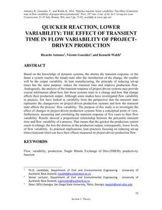
8. Ricardo Antunes, Vicente González, and Kenneth Walsh
80 Proceedings IGLC-24, July 2016 | Boston, USA
Figure 3 shows the step response of production functions shown in Table 2, Cases 1, 4, 5,
3, and 2.
Figure 3 - Transient analysis of Case 1, Case 4, Case 5, Case 3, and Case 2
Table 2 shows the production functions, in the time domain, obtained in for the cases and
used in the transient analysis, sorted in the same order as Table 1.
0 2 4 6 8 10
t [Time (hours)]
0
0.2
0.4
0.6
0.8
1
1.2
y[Actualdepth(meters)]
Case 1: Step response
Steady-state: 1.01 meters
Settling time: 4.67 hours
0 5 10 15 20 25 30
t [Time (days)]
0
0.1
0.2
0.3
0.4
0.5
0.6
0.7
0.8
0.9
1
y[Activityprogress(%)]
Case 4: Step response
Steady-state: 0.99 %
Settling time: 13.11 days
0 0.2 0.4 0.6 0.8 1 1.2 1.4 1.6
t [Time (weeks)]
0
2
4
6
8
10
12
14
16
18
20
y[Productivity(sqrmeters)]
Case 5: Step response
Steady-state: 20.20 sqr meters
Settling time: 1.23 weeks
0 0.5 1 1.5 2 2.5 3 3.5 4
t [Time (weeks)]
0
0.5
1
1.5
2
y[Productivity(sqrmeters)]
Case 3: Step response
Steady-state: 2.21 sqr meters
Settling time: 1.82 weeks
0 20 40 60 80 100 120
t [Time (days)]
0
0.2
0.4
0.6
0.8
1
1.2
1.4
1.6
y[Productivity(sqrmeters)]
Case 2: Step response
Steady-state: 1.00 sqr meters
Settling time: 55.85 days

9. Quicker Reaction, Lower Variability: The Effect of Transient Time in Flow Variability of Project-Driven
Production
Section 1: Theory 81
Table 2 - Productivity Functions
Case Productivity Function
1
4
5
3
2
CONCLUSION
Results show a proportional relationship between the percentile transient time and flow
variability of a process, confirmed by the coefficient of variation and process capability
index calculations. These findings thus lend support that the quicker the production
system reacts to change; the less is the distress in the production output, consequently,
lower levels of flow variability. The findings align with what is known about dynamic
systems and operations management. In manufacturing, the larger the batch, the more
efficient the production process becomes. A larger batch requires a longer run time,
hence the more irrelevant the setup time becomes when compared to the total run time.
The same behavior was observed in construction when calculated the processes’
Percentile reaction time using productivity functions. However, in project-driven
processes increase the batch size and run times are not desired. Increased batch sizes
imply producing more than what is needed: scope creep. That is the muda of over-
production. Prolonged run times translates into extended activities duration. If the scope
is constant the work should be done at a slower peace: decrease of productivity. Hence,
the likely option is to reduce the time spent on the startup (transient time). In this fashion,
productivity functions may provide a way to measure, visualize and compare the transient
state of project-driven processes. Reliance on this method must be tempered, however,
because the number of cases analyzed was small. Therefore, it would be beneficial to
replicate this method in additional cases of project-driven systems in construction. As
practical implications, the understanding of the effects of the transient state on the
process variability may induce practitioners to re-evaluate the application of some Lean
practices in construction. For instance, SMED practices that focus on reducing set-up
times (transient time) can have their effects measured on project-driven production flow
supporting a quantitative and structured application of this method.
P1(t) = 0.8417e 0.8369t
P4 (t) = 0.2955e 0.2984t
P5 (t) = 7.142275814e 3.444656802t
+19.74 t( ) 54.39107581e 33.6753432t
P3(t) =1.455 t( )+1.635385e 2.153t
P2 (t) =1.699 t( ) 0.04910796e 0.07004t

10. Ricardo Antunes, Vicente González, and Kenneth Walsh
82 Proceedings IGLC-24, July 2016 | Boston, USA
REFERENCES
Abdel-Razek, R. H., Elshakour, H. A., and Abdel-Hamid, M. (2007). Labor
productivity: Benchmarking and variability in Egyptian projects. International Journal of
Project Management, 25(2), 189-197. doi:10.1016/j.ijproman.2006.06.001
Antunes, R., and Gonzalez, V. (2015). A production model for construction: A
theoretical framework. Buildings, 5(1), 209-228. doi:10.3390/buildings5010209
Antunes, R., González, V. A., and Walsh, K. (2015, 28-31 July). Identification of
repetitive processes at steady- and unsteady-state: Transfer function. Paper presented at
the 23rd Annual Conference of the International Group for Lean Construction, Perth,
Australia. doi:10.13140/RG.2.1.4193.7364.
Cakmakci, M. (2008). Process improvement: performance analysis of the setup
time reduction-SMED in the automobile industry. The International Journal of Advanced
Manufacturing Technology, 41(1), 168-179. doi:10.1007/s00170-008-1434-4
Gibb, A. G. F. (1999). Off-site Fabrication: Prefabrication, Pre-assembly and
Modularisation: John Wiley and Sons.
Gilbreth, F. B. (1911). Motion study; a method for increasing the efficiency of the
workman. New York: Van Nostrand.
González, V., Alarcón, L. F., Maturana, S., Mundaca, F., and Bustamante, J.
(2010). Improving planning reliability and project performance using the Reliable
Commitment Model. Journal of Construction Engineering and Management, 136(10),
1129-1139. doi:10.1061/(ASCE)CO.1943-7862.0000215
Hayes, R. H., and Wheelwright, S. C. (1979). Link manufacturing process and
product life cycles. Harvard Business Review, 57(1), 133-140
Hopp, W. J., and Spearman, M. L. (2001). Factory physics: Foundations of
manufacturing management (2nd ed.). Boston, MA: Irwin McGraw-Hill.
Montgomery, D. C. (2009). Introduction to statistical quality control (6th ed.).
Hoboken, N.J.: Wiley.
Ohno, T. (1988). O sistema toyota de produção além da produção em larga escala
[Toyota production system: Beyond large-scale production]. Sao Paolo, Brazil:
Bookman.
Shingō, S. (1985). A revolution in manufacturing: the SMED system. Stamford,
CT: Productivity Press.
Taylor, F. W. (1911). The principles of scientific management. New York,
London,: Harper and Brothers.
Womack, J. P., Jones, D. T., and Roos, D. (1991). The machine that changed the
world. New York, NY: Harper Perennial.