SlideShare a Scribd company logo
1 of 13
Unit-2
Probability:-
Probability is “How likely something is to happen” or “chance of occurring of an
event”.
Many events can't be predicted with total certainty. The bestwe can say is how
likely they are to happen, using the idea of probability.
Tossing a Coin when a coin is tossed, there are two possible
outcomes: heads (H) or tails (T).
We say that the probability of the coin landing H is ½.
And the probability of the coin landing T is ½.
Throwing Dice
When a single die is thrown, there are six possible
outcomes: 1, 2, 3, 4, 5, 6.
The probability of any one of them is 1/6.
Probability In general:
𝑃𝑟𝑜𝑏𝑎𝑏𝑖𝑙𝑖𝑡𝑦 𝑜𝑓 𝑎𝑛 𝑒𝑣𝑒𝑛𝑡 ℎ𝑎𝑝𝑝𝑒𝑛𝑖𝑛𝑔 =
𝑁𝑢𝑚𝑏𝑒𝑟 𝑜𝑓 𝑤𝑎𝑦𝑠 𝑖𝑡 𝑐𝑎𝑛 ℎ𝑎𝑝𝑝𝑒𝑛
𝑇𝑜𝑡𝑎𝑙 𝑛𝑢𝑚𝑏𝑒𝑟 𝑜𝑓 𝑜𝑢𝑡𝑐𝑜𝑚𝑒𝑠
Example:The chances of rolling a "4" with a die.
Number of ways it can happen: 1 (there is only 1 face with a "4" on it)
Total number of outcomes: 6 (there are 6 faces altogether)
So the probability =
1
6
Example:There are 5 marbles in a bag: 4 are blue, and 1 is red. Whatis the
probability that a blue marble gets picked?
Number of ways it can happen: 4 (there are 4 blues)
Total number of outcomes: 5 (there are 5 marbles in total)
So the probability =
4
5
= 0.8
Note:-
 Probability is always between 0 and 1
 Probability is Just a Guide
(Probability does not tell us exactly whatwill happen, it is justa guide)
Example:Toss a coin 100 times, how many Heads will come up?
Probability says that heads have a ½ chance, so we can expect 50 Heads.
But when we actually try it we might get 48 heads, or 55 heads ... or anything
really, but in most cases it will be a number near 50.
Some words havespecial meaning in Probability:
Experiment or Trial: an action where the result is uncertain.
Tossing a coin, throwing dice, seeing whatpizza people chooseare all examples of
experiments.
Sample Space: all the possibleoutcomes of an experiment
Example:choosing a card froma deck
There are 52 cards in a deck (not including Jokers)
So the Sample Space is all 52 possiblecards: {Ace of Hearts, 2 of Hearts, etc... }
The Sample Space is made up of Sample Points:
Sample Point: justone of the possible outcomes
Example:Deck of Cards, the 5 of Clubs is a sample point the King of Hearts is a
sample point "King" is not a sample point.
As there are 4 Kings, that is 4 different sample points.
Event:a single result of an experiment
Example Events: Getting a Tail when tossing a coin is an event Rolling a "5" is an
event.
An event can include one or more possibleoutcomes:
Choosing a "King" froma deck of cards (any of the 4 Kings) is an event
Rolling an "even number" (2, 4 or 6) is also an event
The Sample Space is all possibleoutcomes.
A Sample Point is justone possibleoutcome.
And an Event can be one or more of the
possibleoutcomes.
Hey, let's usethose words, so we get used to them:
Example:Alex wants to see how many times a "double" comes up when throwing
2 dice.
Each time Alex throws the 2 dice is an Experiment.
Itis an Experiment becausethe resultis uncertain.
The Event Alex is looking for is a "double", whereboth dice havethe same
number. Itis made up of these 6 Sample Points:
{1,1} {2,2} {3,3} {4,4} {5,5} and {6,6}
The Sample Space is all possibleoutcomes (36 Sample Points):
{1,1} {1,2} {1,3} {1,4} ... {6,3} {6,4} {6,5} {6,6}
These are Alex's Results:
Experiment
Is it a
Double?
{3,4} No
{5,1} No
{2,2} Yes
{6,3} No
... ...
After 100 Experiments, Alex has 19 "double" Events ... is that close to what you
would expect?
Dependent Events:-
Event A and B in the sample spaceS are said to be independent if occurrenceof
one of them does not influence the occurrenceof the other.
i.e. B is dependent of A if P(B/A)=P(B)
Now, P(A∩B)=P(A).P(B|A)=P(A)P(B)
Thus events A and B are independent, if P(A∩B)=P(A).P(B)
Conditional Probabiliry:-
Given an event B such that P(B)>0 and any other event A, we define a conditional
probability of A is given by
𝑃( 𝐴| 𝐵) =
𝑃(𝐴 ∩ 𝐵)
𝑃(𝐵)
Example: Let a balanced die is tossed once. Use the definition to find the
probability of getting 1, given that an odd number was obtained.
Solution:-
Probability of A given that the event B has occurred,
𝑃( 𝐴| 𝐵) =
𝑃(𝐴∩𝐵)
𝑃(𝐵)
But 𝑃( 𝐵) =
1
2
,
𝑃( 𝐴| 𝐵) =
𝑃(𝐴∩𝐵)
𝑃(𝐵)
=
1
6
1
2
=
1
3
.
Law of Total Probability
Let 𝐵1, 𝐵2, …𝐵𝑛 be mutually exclusive and let an event A occur only if anyoneof
𝐵𝑖 occurs, Then 𝑃( 𝐴) = ∑ 𝑃(𝐴|𝐵𝑖)𝑃(𝐵𝑖)𝑛
𝑖=1
Baye’s Theorem
Let 𝐸1, 𝐸2, …𝐸 𝑛 be mutually exclusive event such that 𝑃( 𝐸𝑖) > 0 for each i.
Then for any event 𝐴 ⊆ ⋃ 𝐸𝑖
𝑛
1 such that 𝑃( 𝐴) > 0, we have
𝑃( 𝐸𝑖|𝐴) =
𝑃(𝐴|𝐸𝑖)𝑃(𝐸𝑖)
∑ 𝑃(𝐴|𝐸𝑖)𝑃(𝐸𝑖)𝑛
𝑖=1
𝑖 = 1,2,… 𝑛
Example:- Three urns A, B, C have 1 white , 2 black, 3 red balls, 2 white 1 black, 1
red balls and 4 white
Example:- Let P be the probability that a man aged y years will meet with an
accident in a year. What is the probability that a man among n men all aged y
years will meet with an accident ?
Solution:-
Probability that a man aged y years will not meet with an accident =1-p
P (none meet with an accident) =(1 − 𝑝)(1 − 𝑝)… 𝑛 𝑡𝑖𝑚𝑒𝑠 = (1 − 𝑝) 𝑛
∴ p (atleast one man meets with an accident) = 1 − (1 − 𝑝) 𝑛
So p( atleast one man meets with an accident, a person is chosen)
=
1
𝑛
[1 − (1 − 𝑝) 𝑛]
Example:-
A box contains 4 white, 3 blue and 5 green balls. Four balls are chosen. What is
the probability that all three colors are represented ?
Solution:- The total number of balls in the box is 12.
Hence the total number of ways in which 4 balls can be chosen
= 12
𝐶4 =
12× 11 × 10 × 9
4 × 3 × 2 × 1
= 495
Each color will be represented in the following mutually exclusive ways:
White Blue Green
(i) 2 1 1
(ii) 1 2 1
(iii) 1 1 2
Hence the number of ways of drawing four balls in the abovefashion
= 4
𝐶2 × 3
𝐶1 × 5
𝐶1 + 4
𝐶1 × 3
𝐶2 × 5
𝐶1 + 4
𝐶1 × 3
𝐶1 × 5
𝐶2
= 90 + 60 + 120 = 270
So Required Probability =
270
495
.
Random variable:- A variable whosevalueis determined by the outcome of
randomexperiment is called randomvariable.
The value of the randomvariable will vary fromtrial to trial as the experiment is
repeated. Random variable is also called chance variableor stochastic variable.
There are two types of random variable - discrete and continuous.
A random variable has either an associated probability distribution (discrete random
variable) or probability density function (continuous random variable).
Discrete randomvariable:-
If the random variable takes on the integer values such as 0,1,2, … then it is called
discrete random variable.
Example:-
1. The number in printing mistake in a book, the number of telephone calls
received by the phone operator on a farm areexample of discrete random
variable
2. A coin is tossed ten times. The randomvariable X is the number of tails that
are noted. X can only take the values 0, 1, ..., 10, so X is a discrete random
variable.
Continuous random variable:-
If the randomvariable takes all values, with in a certain interval, then the random
is called continuous randomvariable.
Example:-
1. The amount of rainfall on a rainy day or in a rainy season, the height and
weight of individuals are example of continuous randomvariable.
2. A light bulb is burned until it burns out. The randomvariable Y is its lifetime
in hours. Y can take any positive real value, so Y is a continuous random
variable.
Probability Distribution
The probability distribution of a discrete randomvariable is a list of probabilities
associated with each of its possiblevalues. Itis also sometimes called the
probability function or the probability mass function.
More formally,
In terms of symbols if a variableX can assumediscrete set of values 𝑥1, 𝑥2, … 𝑥 𝑘
with respective probabilities 𝑃1, 𝑃2, … 𝑃𝑘 where 𝑃1 + 𝑃2 + …+ 𝑃𝑘 = 1,
we say that a discrete probability distribution for 𝑋 has been defined.
The function 𝑃(𝑋) which has the respectivevalues 𝑃1 , 𝑃2 , … 𝑃𝑘 for
𝑋 = 𝑥1, 𝑥2,… 𝑥 𝑘 is called the probability function or frequency function of 𝑋.
Note:-
a. 0 ≤ 𝑃(𝑥𝑖) ≤ 1
b. ∑𝑃( 𝑥𝑖) = 1
ExpectedValue:-
The expected value (or population mean) of a randomvariable indicates its
averageor central value. Itis a useful summary value (a number) of the variable's
distribution.
Stating the expected value gives a general impression of the behavior of some
randomvariable without giving full details of its probability distribution (if it is
discrete) or its probability density function (if it is continuous).
Two randomvariables with the same expected value can havevery different
distributions. There are other usefuldescriptivemeasures which affect the shape
of the distribution, for example variance.
The expected value of a randomvariable X is symbolized by E(X) or µ.
If 𝑋 is a discrete randomvariable with possible values 𝑎1, 𝑎2,… 𝑎 𝑘 with respective
probabilities 𝑃1 , 𝑃2 ,… 𝑃𝑘 where 𝑃1 + 𝑃2 + …+ 𝑃𝑘 =1the mathematical
expectation of 𝑋 is defined as:
𝜇 = 𝐸( 𝑋) = ∑ 𝑋(𝑎𝑖)𝑃(𝑎𝑖)
Where the elements are summed over all values of the randomvariable X.
If X is a continuous randomvariablewith probability density function f(x), then
the expected value of X is defined by:
𝜇 = 𝐸( 𝑋) = ∫ 𝑥𝑓( 𝑥) 𝑑𝑥
Example
Discrete case: When a die is thrown, each of the possiblefaces 1, 2, 3, 4, 5, 6 (the
𝑥𝑖's) has a probability of 1/6 (the 𝑃(𝑥𝑖)'s) of showing. Theexpected value of the
face showing is therefore:
µ = 𝐸( 𝑋) = (1 ×
1
6
) + (2 ×
1
6
) + (3 ×
1
6
) + (4 ×
1
6
)
+ (5 ×
1
6
) + (6 ×
1
6
) = 3.5
Notice that, in this case, 𝐸(𝑋) is 3.5, which is not a possiblevalue of 𝑋.
Variance of 𝑋 = 𝑉𝑎𝑟( 𝑋) = 𝜎2
= 𝐸( 𝑋2) − [ 𝐸(𝑋)]2
Standard Deviationof 𝑿 = 𝝈
Example:-
Find expectation of the number of points when a fair die is rolled.
Solution:-
Let 𝑋 be the randomvariable showing number of points. Then 𝑋 = 1,2,3,4,5,6
𝑎𝑖 𝑃(𝑋 = 𝑎𝑖) = 𝑃(𝑎𝑖) Product
1
1
6
1
6
2
1
6
2
6
3
1
6
3
6
4
1
6
4
6
5
1
6
5
6
6
1
6
6
6
________________
𝐸( 𝑋) =
21
6
=
7
2
Expectation =
7
2
.
Normal Distribution
In probability theory, the normal (or Gaussian) distribution is a very commonly
occurring continuous probability distribution .
Strictly, a Normalrandomvariable should be capable of assuming any valueon
the real line, though this requirement is often waived in practice. For example,
height at a given age for a given gender in a given racial group is adequately
described by a Normal randomvariableeven though heights mustbe positive.
A continuous randomvariable X is said to follow a Normal distribution with
parameters µ and 𝜎 if it has probability density function
𝑓( 𝑥) = 𝑓(𝑥, 𝜇, 𝜎 ) =
1
𝜎√2𝜋
𝑒
( 𝑥−𝜇)2
2𝜎2
−∞ ≤ 𝑥 ≤ ∞, 𝜎 > 0,−∞ < 𝜇 < ∞
In such situation we write 𝑋~𝑁( 𝜇, 𝜎2)
The distribution involves two parameters 𝜇 and 𝜎2 .
Properties:-
a) Distribution is symmetrical.
b) 𝑀𝑒𝑎𝑛 = 𝜇, 𝑉𝑎𝑟𝑖𝑎𝑛𝑐𝑒 = 𝜎2 .
c) Mean , median and mode coincide.
d) 𝑓(𝑥) ≥ 0 for all 𝑥.
e) ∫ 𝑥𝑓( 𝑥) 𝑑𝑥
∞
−∞
= 1 i.e. Total area under the curve 𝑦 = 𝑓(𝑥) bounded by the
axix of 𝑥 is 1.
𝑁𝑜𝑡𝑒: −
a) Curvey-f(x), called normal curveis a bell shaped curve.
b) Itis symmetric about 𝑥 = 𝜇.
c) The two tails on the left and right sides of the mean extend to infinity.
d) Put 𝑧 =
𝑥−𝜇
𝜎
. Then 𝑍 is called a standard normalvariable and its
probability density function is given by 𝑃( 𝑧) =
1
√2𝜋
𝑒
−𝑧2
2 ,−∞ ≤ 𝑧 ≤ ∞.
e) Mean of the standard Normaldistributions is 0 and varianceis 1. Write
𝑍~𝑁(0,1)
The simplest case of a normaldistribution is known as the “standard
normaldistribution”.
Areaunder the standard normal curve:-
a) 𝐵𝑒𝑡𝑤𝑒𝑒𝑛 𝑧 = −1 𝑎𝑛𝑑 𝑧 = 1 𝑖𝑠 0.6827(Since total area under the standard
normal curveis 1)
𝑖. 𝑒. 𝑃(−1 < 𝑧 < 1) = 0.6827
b) 𝐵𝑒𝑡𝑤𝑒𝑒𝑛 𝑧 = −2 𝑎𝑛𝑑 𝑧 = 2 𝑖𝑠 0.9595
𝑖. 𝑒. 𝑃(−2 < 𝑧 < 2) = 0.9595
c) 𝐵𝑒𝑡𝑤𝑒𝑒𝑛 𝑧 = −3 𝑎𝑛𝑑 𝑧 = 3 𝑖𝑠 0.9973
𝑖. 𝑒. 𝑃(−3 < 𝑧 > 3) = 0.9973
In other words,
EXAMPLE: If a randomvariable has the normaldistribution with μ = 82.0 and σ=
4.8, Find the probabilities that it will take on a value
(a) less than 89.2
(b) greater than 78.4
(c) between 83.2 and 88.0
(d) between 73.6 and 90.4
Solution:
(a) We have
z =
89.2− 82
4.8
= 1.5
therefore the probability is 0.4332 + 0.5 = 0.9332.
(b) We have
𝑧 =
78.4− 82
4.8
= −0.75
therefore the probability is 0.2734 + 0.5 = 0.7734 .
(c) We have
𝑧1 =
83.2−82
4.8
= 0.25and 𝑧2 =
88−82
4.8
= 1.25
therefore the probability is 0.3944− 0.0987 = 0.2957.
(d) We have 𝑧1 =
73.6−82
4.8
= −1.75and 𝑧2 =
90.4−82
4.8
= 1.75
𝑡hereforethe probability is 0.4599 + 0.4599 = 0.9198.
Applications of the Normal Distribution
EXAMPLE: Intelligence quotients (IQs) measured on the Stanford Revision of the
Binet-Simon Intelligence Scale are normally distributed with a mean of 100 and a
standard deviation of 16.
Determine the percentage of people who haveIQs between 115 and 140.
Solution: We have 𝑧1 =
115−100
16
= 0.9375 and 𝑧2 =
140−100
16
= 2.5
therefore the probability is 0.4938− 0.3264 = 0.1674.
Itfollows that 16.74% of allpeople have IQs between 115 and 140. Equivalently,
the probability is 0.1674 thata randomly selected person will havean IQ between
115 and 140.
Many distribution tend to a normaldistribution in the limit.
When a variable is not normal, it can be made normal using using suitable
transformation.
When the sample size is large distrubution of simple mean, simple variance etc.
approach normality. Thus distribution forms a basis for test of significance.
Normal distribution is also called distribution of errors.
Unit 2 Probability

More Related Content

What's hot

Graphs(Biostatistics and Research Methodology) B.pharmacy(8th sem.)
Graphs(Biostatistics and Research Methodology) B.pharmacy(8th sem.)Graphs(Biostatistics and Research Methodology) B.pharmacy(8th sem.)
Graphs(Biostatistics and Research Methodology) B.pharmacy(8th sem.)Pranjal Saxena
 
Introduction to Research - Biostatistics and Research methodology 8th Sem Uni...
Introduction to Research - Biostatistics and Research methodology 8th Sem Uni...Introduction to Research - Biostatistics and Research methodology 8th Sem Uni...
Introduction to Research - Biostatistics and Research methodology 8th Sem Uni...Himanshu Sharma
 
Probability ,Binomial distribution, Normal distribution, Poisson’s distributi...
Probability ,Binomial distribution, Normal distribution, Poisson’s distributi...Probability ,Binomial distribution, Normal distribution, Poisson’s distributi...
Probability ,Binomial distribution, Normal distribution, Poisson’s distributi...AZCPh
 
Basic stat analysis using excel
Basic stat analysis using excelBasic stat analysis using excel
Basic stat analysis using excelParag Shah
 
Regulatory terminologies used in PV (Pharmacovigilance)
Regulatory terminologies used in PV (Pharmacovigilance)Regulatory terminologies used in PV (Pharmacovigilance)
Regulatory terminologies used in PV (Pharmacovigilance)MubasheeraMg
 
Biostatistics and research methodology
Biostatistics and research methodologyBiostatistics and research methodology
Biostatistics and research methodologysahini kondaviti
 
WHO International Drug Monitoring Program
WHO International Drug Monitoring ProgramWHO International Drug Monitoring Program
WHO International Drug Monitoring ProgramSnehaKhandale1
 
INTERNATIONAL NON PROPRIETARY NAMES FOR DRUGS1.pptx
INTERNATIONAL NON PROPRIETARY NAMES FOR DRUGS1.pptxINTERNATIONAL NON PROPRIETARY NAMES FOR DRUGS1.pptx
INTERNATIONAL NON PROPRIETARY NAMES FOR DRUGS1.pptxE Poovarasan
 
NON-PARAMETRIC TESTS by Prajakta Sawant
NON-PARAMETRIC TESTS by Prajakta SawantNON-PARAMETRIC TESTS by Prajakta Sawant
NON-PARAMETRIC TESTS by Prajakta SawantPRAJAKTASAWANT33
 
Standardized and MedDRA Queries
Standardized and MedDRA QueriesStandardized and MedDRA Queries
Standardized and MedDRA QueriesRajat Garg
 
statistics in pharmaceutical sciences
statistics in pharmaceutical sciencesstatistics in pharmaceutical sciences
statistics in pharmaceutical sciencesTechmasi
 
Introduction to experimental pharmacology
Introduction to experimental pharmacologyIntroduction to experimental pharmacology
Introduction to experimental pharmacologyShaikh Abusufyan
 
Wilcoxon Rank-Sum Test
Wilcoxon Rank-Sum TestWilcoxon Rank-Sum Test
Wilcoxon Rank-Sum TestSahil Jain
 
Biostatics and Research Methodology
Biostatics and Research MethodologyBiostatics and Research Methodology
Biostatics and Research MethodologyShagufta Farooqui
 

What's hot (20)

Graphs(Biostatistics and Research Methodology) B.pharmacy(8th sem.)
Graphs(Biostatistics and Research Methodology) B.pharmacy(8th sem.)Graphs(Biostatistics and Research Methodology) B.pharmacy(8th sem.)
Graphs(Biostatistics and Research Methodology) B.pharmacy(8th sem.)
 
Introduction to Research - Biostatistics and Research methodology 8th Sem Uni...
Introduction to Research - Biostatistics and Research methodology 8th Sem Uni...Introduction to Research - Biostatistics and Research methodology 8th Sem Uni...
Introduction to Research - Biostatistics and Research methodology 8th Sem Uni...
 
Non parametric test
Non parametric testNon parametric test
Non parametric test
 
Probability ,Binomial distribution, Normal distribution, Poisson’s distributi...
Probability ,Binomial distribution, Normal distribution, Poisson’s distributi...Probability ,Binomial distribution, Normal distribution, Poisson’s distributi...
Probability ,Binomial distribution, Normal distribution, Poisson’s distributi...
 
Basic stat analysis using excel
Basic stat analysis using excelBasic stat analysis using excel
Basic stat analysis using excel
 
Regulatory terminologies used in PV (Pharmacovigilance)
Regulatory terminologies used in PV (Pharmacovigilance)Regulatory terminologies used in PV (Pharmacovigilance)
Regulatory terminologies used in PV (Pharmacovigilance)
 
Biostatistics and research methodology
Biostatistics and research methodologyBiostatistics and research methodology
Biostatistics and research methodology
 
Testing of hypothesis
Testing of hypothesisTesting of hypothesis
Testing of hypothesis
 
Biostatistics in Bioequivalence
Biostatistics in BioequivalenceBiostatistics in Bioequivalence
Biostatistics in Bioequivalence
 
WHO International Drug Monitoring Program
WHO International Drug Monitoring ProgramWHO International Drug Monitoring Program
WHO International Drug Monitoring Program
 
INTERNATIONAL NON PROPRIETARY NAMES FOR DRUGS1.pptx
INTERNATIONAL NON PROPRIETARY NAMES FOR DRUGS1.pptxINTERNATIONAL NON PROPRIETARY NAMES FOR DRUGS1.pptx
INTERNATIONAL NON PROPRIETARY NAMES FOR DRUGS1.pptx
 
Pharmacovigilance methods
Pharmacovigilance methodsPharmacovigilance methods
Pharmacovigilance methods
 
Statistical analysis by iswar
Statistical analysis by iswarStatistical analysis by iswar
Statistical analysis by iswar
 
Safety Data Generation
Safety Data GenerationSafety Data Generation
Safety Data Generation
 
NON-PARAMETRIC TESTS by Prajakta Sawant
NON-PARAMETRIC TESTS by Prajakta SawantNON-PARAMETRIC TESTS by Prajakta Sawant
NON-PARAMETRIC TESTS by Prajakta Sawant
 
Standardized and MedDRA Queries
Standardized and MedDRA QueriesStandardized and MedDRA Queries
Standardized and MedDRA Queries
 
statistics in pharmaceutical sciences
statistics in pharmaceutical sciencesstatistics in pharmaceutical sciences
statistics in pharmaceutical sciences
 
Introduction to experimental pharmacology
Introduction to experimental pharmacologyIntroduction to experimental pharmacology
Introduction to experimental pharmacology
 
Wilcoxon Rank-Sum Test
Wilcoxon Rank-Sum TestWilcoxon Rank-Sum Test
Wilcoxon Rank-Sum Test
 
Biostatics and Research Methodology
Biostatics and Research MethodologyBiostatics and Research Methodology
Biostatics and Research Methodology
 

Similar to Unit 2 Probability

Rishabh sehrawat probability
Rishabh sehrawat probabilityRishabh sehrawat probability
Rishabh sehrawat probabilityRishabh Sehrawat
 
Mba i qt unit-4.1_introduction to probability distributions
Mba i qt unit-4.1_introduction to probability distributionsMba i qt unit-4.1_introduction to probability distributions
Mba i qt unit-4.1_introduction to probability distributionsRai University
 
vinayjoshi-131204045346-phpapp02.pdf
vinayjoshi-131204045346-phpapp02.pdfvinayjoshi-131204045346-phpapp02.pdf
vinayjoshi-131204045346-phpapp02.pdfsanjayjha933861
 
Recap_Of_Probability.pptx
Recap_Of_Probability.pptxRecap_Of_Probability.pptx
Recap_Of_Probability.pptxssuseree099d2
 
Discrete Probability Distributions
Discrete Probability DistributionsDiscrete Probability Distributions
Discrete Probability Distributionsmandalina landy
 
Introduction to probability distributions-Statistics and probability analysis
Introduction to probability distributions-Statistics and probability analysis Introduction to probability distributions-Statistics and probability analysis
Introduction to probability distributions-Statistics and probability analysis Vijay Hemmadi
 
SAMPLE SPACES and PROBABILITY (3).pptx
SAMPLE SPACES and PROBABILITY (3).pptxSAMPLE SPACES and PROBABILITY (3).pptx
SAMPLE SPACES and PROBABILITY (3).pptxvictormiralles2
 
PROBABILITY
PROBABILITYPROBABILITY
PROBABILITYVIV13
 
2 Review of Statistics. 2 Review of Statistics.
2 Review of Statistics. 2 Review of Statistics.2 Review of Statistics. 2 Review of Statistics.
2 Review of Statistics. 2 Review of Statistics.WeihanKhor2
 
Probability By Ms Aarti
Probability By Ms AartiProbability By Ms Aarti
Probability By Ms Aartikulachihansraj
 
Indefinite integration class 12
Indefinite integration class 12Indefinite integration class 12
Indefinite integration class 12nysa tutorial
 

Similar to Unit 2 Probability (20)

5. Probability.pdf
5. Probability.pdf5. Probability.pdf
5. Probability.pdf
 
Probability[1]
Probability[1]Probability[1]
Probability[1]
 
Probability
ProbabilityProbability
Probability
 
Probablity ppt maths
Probablity ppt mathsProbablity ppt maths
Probablity ppt maths
 
Probability..
Probability..Probability..
Probability..
 
Rishabh sehrawat probability
Rishabh sehrawat probabilityRishabh sehrawat probability
Rishabh sehrawat probability
 
Mba i qt unit-4.1_introduction to probability distributions
Mba i qt unit-4.1_introduction to probability distributionsMba i qt unit-4.1_introduction to probability distributions
Mba i qt unit-4.1_introduction to probability distributions
 
vinayjoshi-131204045346-phpapp02.pdf
vinayjoshi-131204045346-phpapp02.pdfvinayjoshi-131204045346-phpapp02.pdf
vinayjoshi-131204045346-phpapp02.pdf
 
PROBABILITY.pptx
PROBABILITY.pptxPROBABILITY.pptx
PROBABILITY.pptx
 
Probability.pdf
Probability.pdfProbability.pdf
Probability.pdf
 
Recap_Of_Probability.pptx
Recap_Of_Probability.pptxRecap_Of_Probability.pptx
Recap_Of_Probability.pptx
 
Discrete Probability Distributions
Discrete Probability DistributionsDiscrete Probability Distributions
Discrete Probability Distributions
 
Introduction to probability distributions-Statistics and probability analysis
Introduction to probability distributions-Statistics and probability analysis Introduction to probability distributions-Statistics and probability analysis
Introduction to probability distributions-Statistics and probability analysis
 
lecture4.ppt
lecture4.pptlecture4.ppt
lecture4.ppt
 
SAMPLE SPACES and PROBABILITY (3).pptx
SAMPLE SPACES and PROBABILITY (3).pptxSAMPLE SPACES and PROBABILITY (3).pptx
SAMPLE SPACES and PROBABILITY (3).pptx
 
PROBABILITY
PROBABILITYPROBABILITY
PROBABILITY
 
2 Review of Statistics. 2 Review of Statistics.
2 Review of Statistics. 2 Review of Statistics.2 Review of Statistics. 2 Review of Statistics.
2 Review of Statistics. 2 Review of Statistics.
 
Probability By Ms Aarti
Probability By Ms AartiProbability By Ms Aarti
Probability By Ms Aarti
 
603-probability mj.pptx
603-probability mj.pptx603-probability mj.pptx
603-probability mj.pptx
 
Indefinite integration class 12
Indefinite integration class 12Indefinite integration class 12
Indefinite integration class 12
 

More from Rai University

Brochure Rai University
Brochure Rai University Brochure Rai University
Brochure Rai University Rai University
 
Bdft ii, tmt, unit-iii, dyeing & types of dyeing,
Bdft ii, tmt, unit-iii,  dyeing & types of dyeing,Bdft ii, tmt, unit-iii,  dyeing & types of dyeing,
Bdft ii, tmt, unit-iii, dyeing & types of dyeing,Rai University
 
Bsc agri 2 pae u-4.4 publicrevenue-presentation-130208082149-phpapp02
Bsc agri  2 pae  u-4.4 publicrevenue-presentation-130208082149-phpapp02Bsc agri  2 pae  u-4.4 publicrevenue-presentation-130208082149-phpapp02
Bsc agri 2 pae u-4.4 publicrevenue-presentation-130208082149-phpapp02Rai University
 
Bsc agri 2 pae u-4.3 public expenditure
Bsc agri  2 pae  u-4.3 public expenditureBsc agri  2 pae  u-4.3 public expenditure
Bsc agri 2 pae u-4.3 public expenditureRai University
 
Bsc agri 2 pae u-4.2 public finance
Bsc agri  2 pae  u-4.2 public financeBsc agri  2 pae  u-4.2 public finance
Bsc agri 2 pae u-4.2 public financeRai University
 
Bsc agri 2 pae u-4.1 introduction
Bsc agri  2 pae  u-4.1 introductionBsc agri  2 pae  u-4.1 introduction
Bsc agri 2 pae u-4.1 introductionRai University
 
Bsc agri 2 pae u-3.3 inflation
Bsc agri  2 pae  u-3.3  inflationBsc agri  2 pae  u-3.3  inflation
Bsc agri 2 pae u-3.3 inflationRai University
 
Bsc agri 2 pae u-3.2 introduction to macro economics
Bsc agri  2 pae  u-3.2 introduction to macro economicsBsc agri  2 pae  u-3.2 introduction to macro economics
Bsc agri 2 pae u-3.2 introduction to macro economicsRai University
 
Bsc agri 2 pae u-3.1 marketstructure
Bsc agri  2 pae  u-3.1 marketstructureBsc agri  2 pae  u-3.1 marketstructure
Bsc agri 2 pae u-3.1 marketstructureRai University
 
Bsc agri 2 pae u-3 perfect-competition
Bsc agri  2 pae  u-3 perfect-competitionBsc agri  2 pae  u-3 perfect-competition
Bsc agri 2 pae u-3 perfect-competitionRai University
 

More from Rai University (20)

Brochure Rai University
Brochure Rai University Brochure Rai University
Brochure Rai University
 
Mm unit 4point2
Mm unit 4point2Mm unit 4point2
Mm unit 4point2
 
Mm unit 4point1
Mm unit 4point1Mm unit 4point1
Mm unit 4point1
 
Mm unit 4point3
Mm unit 4point3Mm unit 4point3
Mm unit 4point3
 
Mm unit 3point2
Mm unit 3point2Mm unit 3point2
Mm unit 3point2
 
Mm unit 3point1
Mm unit 3point1Mm unit 3point1
Mm unit 3point1
 
Mm unit 2point2
Mm unit 2point2Mm unit 2point2
Mm unit 2point2
 
Mm unit 2 point 1
Mm unit 2 point 1Mm unit 2 point 1
Mm unit 2 point 1
 
Mm unit 1point3
Mm unit 1point3Mm unit 1point3
Mm unit 1point3
 
Mm unit 1point2
Mm unit 1point2Mm unit 1point2
Mm unit 1point2
 
Mm unit 1point1
Mm unit 1point1Mm unit 1point1
Mm unit 1point1
 
Bdft ii, tmt, unit-iii, dyeing & types of dyeing,
Bdft ii, tmt, unit-iii,  dyeing & types of dyeing,Bdft ii, tmt, unit-iii,  dyeing & types of dyeing,
Bdft ii, tmt, unit-iii, dyeing & types of dyeing,
 
Bsc agri 2 pae u-4.4 publicrevenue-presentation-130208082149-phpapp02
Bsc agri  2 pae  u-4.4 publicrevenue-presentation-130208082149-phpapp02Bsc agri  2 pae  u-4.4 publicrevenue-presentation-130208082149-phpapp02
Bsc agri 2 pae u-4.4 publicrevenue-presentation-130208082149-phpapp02
 
Bsc agri 2 pae u-4.3 public expenditure
Bsc agri  2 pae  u-4.3 public expenditureBsc agri  2 pae  u-4.3 public expenditure
Bsc agri 2 pae u-4.3 public expenditure
 
Bsc agri 2 pae u-4.2 public finance
Bsc agri  2 pae  u-4.2 public financeBsc agri  2 pae  u-4.2 public finance
Bsc agri 2 pae u-4.2 public finance
 
Bsc agri 2 pae u-4.1 introduction
Bsc agri  2 pae  u-4.1 introductionBsc agri  2 pae  u-4.1 introduction
Bsc agri 2 pae u-4.1 introduction
 
Bsc agri 2 pae u-3.3 inflation
Bsc agri  2 pae  u-3.3  inflationBsc agri  2 pae  u-3.3  inflation
Bsc agri 2 pae u-3.3 inflation
 
Bsc agri 2 pae u-3.2 introduction to macro economics
Bsc agri  2 pae  u-3.2 introduction to macro economicsBsc agri  2 pae  u-3.2 introduction to macro economics
Bsc agri 2 pae u-3.2 introduction to macro economics
 
Bsc agri 2 pae u-3.1 marketstructure
Bsc agri  2 pae  u-3.1 marketstructureBsc agri  2 pae  u-3.1 marketstructure
Bsc agri 2 pae u-3.1 marketstructure
 
Bsc agri 2 pae u-3 perfect-competition
Bsc agri  2 pae  u-3 perfect-competitionBsc agri  2 pae  u-3 perfect-competition
Bsc agri 2 pae u-3 perfect-competition
 

Recently uploaded

Industrial Policy - 1948, 1956, 1973, 1977, 1980, 1991
Industrial Policy - 1948, 1956, 1973, 1977, 1980, 1991Industrial Policy - 1948, 1956, 1973, 1977, 1980, 1991
Industrial Policy - 1948, 1956, 1973, 1977, 1980, 1991RKavithamani
 
Sanyam Choudhary Chemistry practical.pdf
Sanyam Choudhary Chemistry practical.pdfSanyam Choudhary Chemistry practical.pdf
Sanyam Choudhary Chemistry practical.pdfsanyamsingh5019
 
Measures of Central Tendency: Mean, Median and Mode
Measures of Central Tendency: Mean, Median and ModeMeasures of Central Tendency: Mean, Median and Mode
Measures of Central Tendency: Mean, Median and ModeThiyagu K
 
Privatization and Disinvestment - Meaning, Objectives, Advantages and Disadva...
Privatization and Disinvestment - Meaning, Objectives, Advantages and Disadva...Privatization and Disinvestment - Meaning, Objectives, Advantages and Disadva...
Privatization and Disinvestment - Meaning, Objectives, Advantages and Disadva...RKavithamani
 
The Most Excellent Way | 1 Corinthians 13
The Most Excellent Way | 1 Corinthians 13The Most Excellent Way | 1 Corinthians 13
The Most Excellent Way | 1 Corinthians 13Steve Thomason
 
Accessible design: Minimum effort, maximum impact
Accessible design: Minimum effort, maximum impactAccessible design: Minimum effort, maximum impact
Accessible design: Minimum effort, maximum impactdawncurless
 
Web & Social Media Analytics Previous Year Question Paper.pdf
Web & Social Media Analytics Previous Year Question Paper.pdfWeb & Social Media Analytics Previous Year Question Paper.pdf
Web & Social Media Analytics Previous Year Question Paper.pdfJayanti Pande
 
The basics of sentences session 2pptx copy.pptx
The basics of sentences session 2pptx copy.pptxThe basics of sentences session 2pptx copy.pptx
The basics of sentences session 2pptx copy.pptxheathfieldcps1
 
Hybridoma Technology ( Production , Purification , and Application )
Hybridoma Technology  ( Production , Purification , and Application  ) Hybridoma Technology  ( Production , Purification , and Application  )
Hybridoma Technology ( Production , Purification , and Application ) Sakshi Ghasle
 
SOCIAL AND HISTORICAL CONTEXT - LFTVD.pptx
SOCIAL AND HISTORICAL CONTEXT - LFTVD.pptxSOCIAL AND HISTORICAL CONTEXT - LFTVD.pptx
SOCIAL AND HISTORICAL CONTEXT - LFTVD.pptxiammrhaywood
 
“Oh GOSH! Reflecting on Hackteria's Collaborative Practices in a Global Do-It...
“Oh GOSH! Reflecting on Hackteria's Collaborative Practices in a Global Do-It...“Oh GOSH! Reflecting on Hackteria's Collaborative Practices in a Global Do-It...
“Oh GOSH! Reflecting on Hackteria's Collaborative Practices in a Global Do-It...Marc Dusseiller Dusjagr
 
Paris 2024 Olympic Geographies - an activity
Paris 2024 Olympic Geographies - an activityParis 2024 Olympic Geographies - an activity
Paris 2024 Olympic Geographies - an activityGeoBlogs
 
Presentation by Andreas Schleicher Tackling the School Absenteeism Crisis 30 ...
Presentation by Andreas Schleicher Tackling the School Absenteeism Crisis 30 ...Presentation by Andreas Schleicher Tackling the School Absenteeism Crisis 30 ...
Presentation by Andreas Schleicher Tackling the School Absenteeism Crisis 30 ...EduSkills OECD
 
POINT- BIOCHEMISTRY SEM 2 ENZYMES UNIT 5.pptx
POINT- BIOCHEMISTRY SEM 2 ENZYMES UNIT 5.pptxPOINT- BIOCHEMISTRY SEM 2 ENZYMES UNIT 5.pptx
POINT- BIOCHEMISTRY SEM 2 ENZYMES UNIT 5.pptxSayali Powar
 
Grant Readiness 101 TechSoup and Remy Consulting
Grant Readiness 101 TechSoup and Remy ConsultingGrant Readiness 101 TechSoup and Remy Consulting
Grant Readiness 101 TechSoup and Remy ConsultingTechSoup
 
Call Girls in Dwarka Mor Delhi Contact Us 9654467111
Call Girls in Dwarka Mor Delhi Contact Us 9654467111Call Girls in Dwarka Mor Delhi Contact Us 9654467111
Call Girls in Dwarka Mor Delhi Contact Us 9654467111Sapana Sha
 
1029-Danh muc Sach Giao Khoa khoi 6.pdf
1029-Danh muc Sach Giao Khoa khoi  6.pdf1029-Danh muc Sach Giao Khoa khoi  6.pdf
1029-Danh muc Sach Giao Khoa khoi 6.pdfQucHHunhnh
 
Kisan Call Centre - To harness potential of ICT in Agriculture by answer farm...
Kisan Call Centre - To harness potential of ICT in Agriculture by answer farm...Kisan Call Centre - To harness potential of ICT in Agriculture by answer farm...
Kisan Call Centre - To harness potential of ICT in Agriculture by answer farm...Krashi Coaching
 

Recently uploaded (20)

INDIA QUIZ 2024 RLAC DELHI UNIVERSITY.pptx
INDIA QUIZ 2024 RLAC DELHI UNIVERSITY.pptxINDIA QUIZ 2024 RLAC DELHI UNIVERSITY.pptx
INDIA QUIZ 2024 RLAC DELHI UNIVERSITY.pptx
 
Industrial Policy - 1948, 1956, 1973, 1977, 1980, 1991
Industrial Policy - 1948, 1956, 1973, 1977, 1980, 1991Industrial Policy - 1948, 1956, 1973, 1977, 1980, 1991
Industrial Policy - 1948, 1956, 1973, 1977, 1980, 1991
 
Sanyam Choudhary Chemistry practical.pdf
Sanyam Choudhary Chemistry practical.pdfSanyam Choudhary Chemistry practical.pdf
Sanyam Choudhary Chemistry practical.pdf
 
Measures of Central Tendency: Mean, Median and Mode
Measures of Central Tendency: Mean, Median and ModeMeasures of Central Tendency: Mean, Median and Mode
Measures of Central Tendency: Mean, Median and Mode
 
Privatization and Disinvestment - Meaning, Objectives, Advantages and Disadva...
Privatization and Disinvestment - Meaning, Objectives, Advantages and Disadva...Privatization and Disinvestment - Meaning, Objectives, Advantages and Disadva...
Privatization and Disinvestment - Meaning, Objectives, Advantages and Disadva...
 
The Most Excellent Way | 1 Corinthians 13
The Most Excellent Way | 1 Corinthians 13The Most Excellent Way | 1 Corinthians 13
The Most Excellent Way | 1 Corinthians 13
 
Accessible design: Minimum effort, maximum impact
Accessible design: Minimum effort, maximum impactAccessible design: Minimum effort, maximum impact
Accessible design: Minimum effort, maximum impact
 
Web & Social Media Analytics Previous Year Question Paper.pdf
Web & Social Media Analytics Previous Year Question Paper.pdfWeb & Social Media Analytics Previous Year Question Paper.pdf
Web & Social Media Analytics Previous Year Question Paper.pdf
 
The basics of sentences session 2pptx copy.pptx
The basics of sentences session 2pptx copy.pptxThe basics of sentences session 2pptx copy.pptx
The basics of sentences session 2pptx copy.pptx
 
Hybridoma Technology ( Production , Purification , and Application )
Hybridoma Technology  ( Production , Purification , and Application  ) Hybridoma Technology  ( Production , Purification , and Application  )
Hybridoma Technology ( Production , Purification , and Application )
 
SOCIAL AND HISTORICAL CONTEXT - LFTVD.pptx
SOCIAL AND HISTORICAL CONTEXT - LFTVD.pptxSOCIAL AND HISTORICAL CONTEXT - LFTVD.pptx
SOCIAL AND HISTORICAL CONTEXT - LFTVD.pptx
 
Código Creativo y Arte de Software | Unidad 1
Código Creativo y Arte de Software | Unidad 1Código Creativo y Arte de Software | Unidad 1
Código Creativo y Arte de Software | Unidad 1
 
“Oh GOSH! Reflecting on Hackteria's Collaborative Practices in a Global Do-It...
“Oh GOSH! Reflecting on Hackteria's Collaborative Practices in a Global Do-It...“Oh GOSH! Reflecting on Hackteria's Collaborative Practices in a Global Do-It...
“Oh GOSH! Reflecting on Hackteria's Collaborative Practices in a Global Do-It...
 
Paris 2024 Olympic Geographies - an activity
Paris 2024 Olympic Geographies - an activityParis 2024 Olympic Geographies - an activity
Paris 2024 Olympic Geographies - an activity
 
Presentation by Andreas Schleicher Tackling the School Absenteeism Crisis 30 ...
Presentation by Andreas Schleicher Tackling the School Absenteeism Crisis 30 ...Presentation by Andreas Schleicher Tackling the School Absenteeism Crisis 30 ...
Presentation by Andreas Schleicher Tackling the School Absenteeism Crisis 30 ...
 
POINT- BIOCHEMISTRY SEM 2 ENZYMES UNIT 5.pptx
POINT- BIOCHEMISTRY SEM 2 ENZYMES UNIT 5.pptxPOINT- BIOCHEMISTRY SEM 2 ENZYMES UNIT 5.pptx
POINT- BIOCHEMISTRY SEM 2 ENZYMES UNIT 5.pptx
 
Grant Readiness 101 TechSoup and Remy Consulting
Grant Readiness 101 TechSoup and Remy ConsultingGrant Readiness 101 TechSoup and Remy Consulting
Grant Readiness 101 TechSoup and Remy Consulting
 
Call Girls in Dwarka Mor Delhi Contact Us 9654467111
Call Girls in Dwarka Mor Delhi Contact Us 9654467111Call Girls in Dwarka Mor Delhi Contact Us 9654467111
Call Girls in Dwarka Mor Delhi Contact Us 9654467111
 
1029-Danh muc Sach Giao Khoa khoi 6.pdf
1029-Danh muc Sach Giao Khoa khoi  6.pdf1029-Danh muc Sach Giao Khoa khoi  6.pdf
1029-Danh muc Sach Giao Khoa khoi 6.pdf
 
Kisan Call Centre - To harness potential of ICT in Agriculture by answer farm...
Kisan Call Centre - To harness potential of ICT in Agriculture by answer farm...Kisan Call Centre - To harness potential of ICT in Agriculture by answer farm...
Kisan Call Centre - To harness potential of ICT in Agriculture by answer farm...
 

Unit 2 Probability

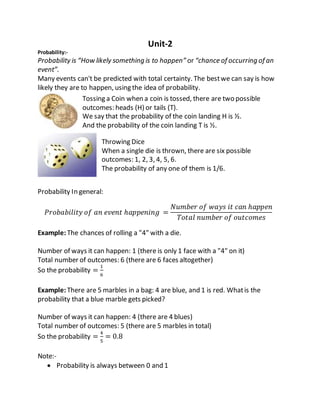
  • 1. Unit-2 Probability:- Probability is “How likely something is to happen” or “chance of occurring of an event”. Many events can't be predicted with total certainty. The bestwe can say is how likely they are to happen, using the idea of probability. Tossing a Coin when a coin is tossed, there are two possible outcomes: heads (H) or tails (T). We say that the probability of the coin landing H is ½. And the probability of the coin landing T is ½. Throwing Dice When a single die is thrown, there are six possible outcomes: 1, 2, 3, 4, 5, 6. The probability of any one of them is 1/6. Probability In general: 𝑃𝑟𝑜𝑏𝑎𝑏𝑖𝑙𝑖𝑡𝑦 𝑜𝑓 𝑎𝑛 𝑒𝑣𝑒𝑛𝑡 ℎ𝑎𝑝𝑝𝑒𝑛𝑖𝑛𝑔 = 𝑁𝑢𝑚𝑏𝑒𝑟 𝑜𝑓 𝑤𝑎𝑦𝑠 𝑖𝑡 𝑐𝑎𝑛 ℎ𝑎𝑝𝑝𝑒𝑛 𝑇𝑜𝑡𝑎𝑙 𝑛𝑢𝑚𝑏𝑒𝑟 𝑜𝑓 𝑜𝑢𝑡𝑐𝑜𝑚𝑒𝑠 Example:The chances of rolling a "4" with a die. Number of ways it can happen: 1 (there is only 1 face with a "4" on it) Total number of outcomes: 6 (there are 6 faces altogether) So the probability = 1 6 Example:There are 5 marbles in a bag: 4 are blue, and 1 is red. Whatis the probability that a blue marble gets picked? Number of ways it can happen: 4 (there are 4 blues) Total number of outcomes: 5 (there are 5 marbles in total) So the probability = 4 5 = 0.8 Note:-  Probability is always between 0 and 1
  • 2.  Probability is Just a Guide (Probability does not tell us exactly whatwill happen, it is justa guide) Example:Toss a coin 100 times, how many Heads will come up? Probability says that heads have a ½ chance, so we can expect 50 Heads. But when we actually try it we might get 48 heads, or 55 heads ... or anything really, but in most cases it will be a number near 50. Some words havespecial meaning in Probability: Experiment or Trial: an action where the result is uncertain. Tossing a coin, throwing dice, seeing whatpizza people chooseare all examples of experiments. Sample Space: all the possibleoutcomes of an experiment Example:choosing a card froma deck There are 52 cards in a deck (not including Jokers) So the Sample Space is all 52 possiblecards: {Ace of Hearts, 2 of Hearts, etc... } The Sample Space is made up of Sample Points: Sample Point: justone of the possible outcomes Example:Deck of Cards, the 5 of Clubs is a sample point the King of Hearts is a sample point "King" is not a sample point. As there are 4 Kings, that is 4 different sample points. Event:a single result of an experiment Example Events: Getting a Tail when tossing a coin is an event Rolling a "5" is an event. An event can include one or more possibleoutcomes: Choosing a "King" froma deck of cards (any of the 4 Kings) is an event Rolling an "even number" (2, 4 or 6) is also an event
  • 3. The Sample Space is all possibleoutcomes. A Sample Point is justone possibleoutcome. And an Event can be one or more of the possibleoutcomes. Hey, let's usethose words, so we get used to them: Example:Alex wants to see how many times a "double" comes up when throwing 2 dice. Each time Alex throws the 2 dice is an Experiment. Itis an Experiment becausethe resultis uncertain. The Event Alex is looking for is a "double", whereboth dice havethe same number. Itis made up of these 6 Sample Points: {1,1} {2,2} {3,3} {4,4} {5,5} and {6,6} The Sample Space is all possibleoutcomes (36 Sample Points): {1,1} {1,2} {1,3} {1,4} ... {6,3} {6,4} {6,5} {6,6} These are Alex's Results: Experiment Is it a Double? {3,4} No {5,1} No {2,2} Yes {6,3} No ... ...
  • 4. After 100 Experiments, Alex has 19 "double" Events ... is that close to what you would expect? Dependent Events:- Event A and B in the sample spaceS are said to be independent if occurrenceof one of them does not influence the occurrenceof the other. i.e. B is dependent of A if P(B/A)=P(B) Now, P(A∩B)=P(A).P(B|A)=P(A)P(B) Thus events A and B are independent, if P(A∩B)=P(A).P(B) Conditional Probabiliry:- Given an event B such that P(B)>0 and any other event A, we define a conditional probability of A is given by 𝑃( 𝐴| 𝐵) = 𝑃(𝐴 ∩ 𝐵) 𝑃(𝐵) Example: Let a balanced die is tossed once. Use the definition to find the probability of getting 1, given that an odd number was obtained. Solution:- Probability of A given that the event B has occurred, 𝑃( 𝐴| 𝐵) = 𝑃(𝐴∩𝐵) 𝑃(𝐵) But 𝑃( 𝐵) = 1 2 , 𝑃( 𝐴| 𝐵) = 𝑃(𝐴∩𝐵) 𝑃(𝐵) = 1 6 1 2 = 1 3 . Law of Total Probability Let 𝐵1, 𝐵2, …𝐵𝑛 be mutually exclusive and let an event A occur only if anyoneof 𝐵𝑖 occurs, Then 𝑃( 𝐴) = ∑ 𝑃(𝐴|𝐵𝑖)𝑃(𝐵𝑖)𝑛 𝑖=1 Baye’s Theorem Let 𝐸1, 𝐸2, …𝐸 𝑛 be mutually exclusive event such that 𝑃( 𝐸𝑖) > 0 for each i. Then for any event 𝐴 ⊆ ⋃ 𝐸𝑖 𝑛 1 such that 𝑃( 𝐴) > 0, we have 𝑃( 𝐸𝑖|𝐴) = 𝑃(𝐴|𝐸𝑖)𝑃(𝐸𝑖) ∑ 𝑃(𝐴|𝐸𝑖)𝑃(𝐸𝑖)𝑛 𝑖=1 𝑖 = 1,2,… 𝑛 Example:- Three urns A, B, C have 1 white , 2 black, 3 red balls, 2 white 1 black, 1 red balls and 4 white Example:- Let P be the probability that a man aged y years will meet with an accident in a year. What is the probability that a man among n men all aged y years will meet with an accident ? Solution:-
  • 5. Probability that a man aged y years will not meet with an accident =1-p P (none meet with an accident) =(1 − 𝑝)(1 − 𝑝)… 𝑛 𝑡𝑖𝑚𝑒𝑠 = (1 − 𝑝) 𝑛 ∴ p (atleast one man meets with an accident) = 1 − (1 − 𝑝) 𝑛 So p( atleast one man meets with an accident, a person is chosen) = 1 𝑛 [1 − (1 − 𝑝) 𝑛] Example:- A box contains 4 white, 3 blue and 5 green balls. Four balls are chosen. What is the probability that all three colors are represented ? Solution:- The total number of balls in the box is 12. Hence the total number of ways in which 4 balls can be chosen = 12 𝐶4 = 12× 11 × 10 × 9 4 × 3 × 2 × 1 = 495 Each color will be represented in the following mutually exclusive ways: White Blue Green (i) 2 1 1 (ii) 1 2 1 (iii) 1 1 2 Hence the number of ways of drawing four balls in the abovefashion = 4 𝐶2 × 3 𝐶1 × 5 𝐶1 + 4 𝐶1 × 3 𝐶2 × 5 𝐶1 + 4 𝐶1 × 3 𝐶1 × 5 𝐶2 = 90 + 60 + 120 = 270 So Required Probability = 270 495 . Random variable:- A variable whosevalueis determined by the outcome of randomexperiment is called randomvariable. The value of the randomvariable will vary fromtrial to trial as the experiment is repeated. Random variable is also called chance variableor stochastic variable. There are two types of random variable - discrete and continuous. A random variable has either an associated probability distribution (discrete random variable) or probability density function (continuous random variable). Discrete randomvariable:- If the random variable takes on the integer values such as 0,1,2, … then it is called discrete random variable.
  • 6. Example:- 1. The number in printing mistake in a book, the number of telephone calls received by the phone operator on a farm areexample of discrete random variable 2. A coin is tossed ten times. The randomvariable X is the number of tails that are noted. X can only take the values 0, 1, ..., 10, so X is a discrete random variable. Continuous random variable:- If the randomvariable takes all values, with in a certain interval, then the random is called continuous randomvariable. Example:- 1. The amount of rainfall on a rainy day or in a rainy season, the height and weight of individuals are example of continuous randomvariable. 2. A light bulb is burned until it burns out. The randomvariable Y is its lifetime in hours. Y can take any positive real value, so Y is a continuous random variable. Probability Distribution The probability distribution of a discrete randomvariable is a list of probabilities associated with each of its possiblevalues. Itis also sometimes called the probability function or the probability mass function. More formally, In terms of symbols if a variableX can assumediscrete set of values 𝑥1, 𝑥2, … 𝑥 𝑘 with respective probabilities 𝑃1, 𝑃2, … 𝑃𝑘 where 𝑃1 + 𝑃2 + …+ 𝑃𝑘 = 1, we say that a discrete probability distribution for 𝑋 has been defined. The function 𝑃(𝑋) which has the respectivevalues 𝑃1 , 𝑃2 , … 𝑃𝑘 for 𝑋 = 𝑥1, 𝑥2,… 𝑥 𝑘 is called the probability function or frequency function of 𝑋. Note:-
  • 7. a. 0 ≤ 𝑃(𝑥𝑖) ≤ 1 b. ∑𝑃( 𝑥𝑖) = 1 ExpectedValue:- The expected value (or population mean) of a randomvariable indicates its averageor central value. Itis a useful summary value (a number) of the variable's distribution. Stating the expected value gives a general impression of the behavior of some randomvariable without giving full details of its probability distribution (if it is discrete) or its probability density function (if it is continuous). Two randomvariables with the same expected value can havevery different distributions. There are other usefuldescriptivemeasures which affect the shape of the distribution, for example variance. The expected value of a randomvariable X is symbolized by E(X) or µ. If 𝑋 is a discrete randomvariable with possible values 𝑎1, 𝑎2,… 𝑎 𝑘 with respective probabilities 𝑃1 , 𝑃2 ,… 𝑃𝑘 where 𝑃1 + 𝑃2 + …+ 𝑃𝑘 =1the mathematical expectation of 𝑋 is defined as: 𝜇 = 𝐸( 𝑋) = ∑ 𝑋(𝑎𝑖)𝑃(𝑎𝑖) Where the elements are summed over all values of the randomvariable X. If X is a continuous randomvariablewith probability density function f(x), then the expected value of X is defined by: 𝜇 = 𝐸( 𝑋) = ∫ 𝑥𝑓( 𝑥) 𝑑𝑥 Example
  • 8. Discrete case: When a die is thrown, each of the possiblefaces 1, 2, 3, 4, 5, 6 (the 𝑥𝑖's) has a probability of 1/6 (the 𝑃(𝑥𝑖)'s) of showing. Theexpected value of the face showing is therefore: µ = 𝐸( 𝑋) = (1 × 1 6 ) + (2 × 1 6 ) + (3 × 1 6 ) + (4 × 1 6 ) + (5 × 1 6 ) + (6 × 1 6 ) = 3.5 Notice that, in this case, 𝐸(𝑋) is 3.5, which is not a possiblevalue of 𝑋. Variance of 𝑋 = 𝑉𝑎𝑟( 𝑋) = 𝜎2 = 𝐸( 𝑋2) − [ 𝐸(𝑋)]2 Standard Deviationof 𝑿 = 𝝈 Example:- Find expectation of the number of points when a fair die is rolled. Solution:- Let 𝑋 be the randomvariable showing number of points. Then 𝑋 = 1,2,3,4,5,6 𝑎𝑖 𝑃(𝑋 = 𝑎𝑖) = 𝑃(𝑎𝑖) Product 1 1 6 1 6 2 1 6 2 6 3 1 6 3 6 4 1 6 4 6 5 1 6 5 6 6 1 6 6 6 ________________ 𝐸( 𝑋) = 21 6 = 7 2 Expectation = 7 2 .
  • 9. Normal Distribution In probability theory, the normal (or Gaussian) distribution is a very commonly occurring continuous probability distribution . Strictly, a Normalrandomvariable should be capable of assuming any valueon the real line, though this requirement is often waived in practice. For example, height at a given age for a given gender in a given racial group is adequately described by a Normal randomvariableeven though heights mustbe positive. A continuous randomvariable X is said to follow a Normal distribution with parameters µ and 𝜎 if it has probability density function 𝑓( 𝑥) = 𝑓(𝑥, 𝜇, 𝜎 ) = 1 𝜎√2𝜋 𝑒 ( 𝑥−𝜇)2 2𝜎2 −∞ ≤ 𝑥 ≤ ∞, 𝜎 > 0,−∞ < 𝜇 < ∞ In such situation we write 𝑋~𝑁( 𝜇, 𝜎2) The distribution involves two parameters 𝜇 and 𝜎2 . Properties:- a) Distribution is symmetrical. b) 𝑀𝑒𝑎𝑛 = 𝜇, 𝑉𝑎𝑟𝑖𝑎𝑛𝑐𝑒 = 𝜎2 .
  • 10. c) Mean , median and mode coincide. d) 𝑓(𝑥) ≥ 0 for all 𝑥. e) ∫ 𝑥𝑓( 𝑥) 𝑑𝑥 ∞ −∞ = 1 i.e. Total area under the curve 𝑦 = 𝑓(𝑥) bounded by the axix of 𝑥 is 1. 𝑁𝑜𝑡𝑒: − a) Curvey-f(x), called normal curveis a bell shaped curve. b) Itis symmetric about 𝑥 = 𝜇. c) The two tails on the left and right sides of the mean extend to infinity. d) Put 𝑧 = 𝑥−𝜇 𝜎 . Then 𝑍 is called a standard normalvariable and its probability density function is given by 𝑃( 𝑧) = 1 √2𝜋 𝑒 −𝑧2 2 ,−∞ ≤ 𝑧 ≤ ∞. e) Mean of the standard Normaldistributions is 0 and varianceis 1. Write 𝑍~𝑁(0,1) The simplest case of a normaldistribution is known as the “standard normaldistribution”. Areaunder the standard normal curve:- a) 𝐵𝑒𝑡𝑤𝑒𝑒𝑛 𝑧 = −1 𝑎𝑛𝑑 𝑧 = 1 𝑖𝑠 0.6827(Since total area under the standard normal curveis 1) 𝑖. 𝑒. 𝑃(−1 < 𝑧 < 1) = 0.6827 b) 𝐵𝑒𝑡𝑤𝑒𝑒𝑛 𝑧 = −2 𝑎𝑛𝑑 𝑧 = 2 𝑖𝑠 0.9595 𝑖. 𝑒. 𝑃(−2 < 𝑧 < 2) = 0.9595 c) 𝐵𝑒𝑡𝑤𝑒𝑒𝑛 𝑧 = −3 𝑎𝑛𝑑 𝑧 = 3 𝑖𝑠 0.9973 𝑖. 𝑒. 𝑃(−3 < 𝑧 > 3) = 0.9973 In other words,
  • 11. EXAMPLE: If a randomvariable has the normaldistribution with μ = 82.0 and σ= 4.8, Find the probabilities that it will take on a value (a) less than 89.2 (b) greater than 78.4 (c) between 83.2 and 88.0 (d) between 73.6 and 90.4 Solution: (a) We have
  • 12. z = 89.2− 82 4.8 = 1.5 therefore the probability is 0.4332 + 0.5 = 0.9332. (b) We have 𝑧 = 78.4− 82 4.8 = −0.75 therefore the probability is 0.2734 + 0.5 = 0.7734 . (c) We have 𝑧1 = 83.2−82 4.8 = 0.25and 𝑧2 = 88−82 4.8 = 1.25 therefore the probability is 0.3944− 0.0987 = 0.2957. (d) We have 𝑧1 = 73.6−82 4.8 = −1.75and 𝑧2 = 90.4−82 4.8 = 1.75 𝑡hereforethe probability is 0.4599 + 0.4599 = 0.9198. Applications of the Normal Distribution EXAMPLE: Intelligence quotients (IQs) measured on the Stanford Revision of the Binet-Simon Intelligence Scale are normally distributed with a mean of 100 and a standard deviation of 16. Determine the percentage of people who haveIQs between 115 and 140. Solution: We have 𝑧1 = 115−100 16 = 0.9375 and 𝑧2 = 140−100 16 = 2.5 therefore the probability is 0.4938− 0.3264 = 0.1674. Itfollows that 16.74% of allpeople have IQs between 115 and 140. Equivalently, the probability is 0.1674 thata randomly selected person will havean IQ between 115 and 140. Many distribution tend to a normaldistribution in the limit. When a variable is not normal, it can be made normal using using suitable transformation. When the sample size is large distrubution of simple mean, simple variance etc. approach normality. Thus distribution forms a basis for test of significance. Normal distribution is also called distribution of errors.