Ch04 se

Introduction to
Relations
and Functions
4.1 Introduction to Relations
4.2 Introduction to Functions
4.3 Graphs of Functions
4.4 Variation
255
In this chapter we introduce the concept of a function. In general terms,
a function defines how one variable depends on one or more other variables.
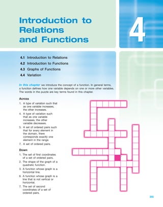
The words in the puzzle are key terms found in this chapter.
Across
1. A type of variation such that
as one variable increases,
the other increases.
4. A type of variation such
that as one variable
increases, the other
variable decreases.
5. A set of ordered pairs such
that for every element in
the domain, there
corresponds exactly one
element in the range.
7. A set of ordered pairs.
Down
1. The set of first coordinates
of a set of ordered pairs.
2. The shape of the graph of a
quadratic function.
3. A function whose graph is a
horizontal line.
6. A function whose graph is a
line that is not vertical or
horizontal.
7. The set of second
coordinates of a set of
ordered pairs.
1
4
2
3
5
6
7
IA
44
miL2872X_ch04_255-308 9/26/06 02:15 PM Page 255
CONFIRMING PAGES

256 Chapter 4 Introduction to Relations and Functions
1. Domain and Range of a Relation
In many naturally occurring phenomena, two variables may be linked by some
type of relationship. For instance, an archeologist finds the bones of a woman
at an excavation site. One of the bones is a femur. The femur is the large bone
in the thigh attached to the knee and hip. Table 4-1 shows a correspondence
between the length of a woman’s femur and her height.
Each data point from Table 4-1 may be represented as an ordered pair. In this
case, the first value represents the length of a woman’s femur and the second,
the woman’s height. The set of ordered pairs {(45.5, 65.5), (48.2, 68.0), (41.8, 62.2),
(46.0, 66.0), (50.4, 70.0)} defines a relation between femur length and height.
Finding the Domain and Range of a Relation
Find the domain and range of the relation linking the length of a woman’s femur
to her height {(45.5, 65.5), (48.2, 68.0), (41.8, 62.2), (46.0, 66.0), (50.4, 70.0)}.
Solution:
Domain: {45.5, 48.2, 41.8, 46.0, 50.4} Set of first coordinates
Range: {65.5, 68.0, 62.2, 66.0, 70.0} Set of second coordinates
1. Find the domain and range of the relation.
e 10, 02, 1Ϫ8, 42, a
1
2
, 1b, 1Ϫ3, 42, 1Ϫ8, 02 f
Skill Practice
Example 1
Table 4-1
Definition of a Relation in x and y
Any set of ordered pairs (x,y) is called a relation in x and y. Furthermore,
• The set of first components in the ordered pairs is called the domain of
the relation.
• The set of second components in the ordered pairs is called the range of
the relation.
Skill Practice Answers
1. Domain
range 50, 4, 16
e0, Ϫ8,
1
2
, Ϫ3f,
Length of Height
Femur (cm) (in.) Ordered Pair
x y
45.5 65.5 (45.5, 65.5)
48.2 68.0 (48.2, 68.0)
41.8 62.2 (41.8, 62.2)
46.0 66.0 (46.0, 66.0)
50.4 70.0 (50.4, 70.0)
Section 4.1 Introduction to Relations
Concepts
1. Domain and Range of a
Relation
2. Applications Involving
Relations
IAmiL2872X_ch04_255-308 9/25/06 11:51 AM Page 256
CONFIRMING PAGES

Section 4.1 Introduction to Relations 257
Find the domain and range of the relation
{(Alabama, 7), (California, 53), (Colorado, 7), (Florida, 25), (Kansas, 4)}
Solution:
Domain: {Alabama, California, Colorado, Florida, Kansas}
Range: {7, 53, 25, 4} (Note: The element 7 is not listed twice.)
2. The table gives the longevity for four types of animals. Write the ordered
pairs (x, y) indicated by this relation, and state the domain and range.
A relation may consist of a finite number of ordered pairs or an infinite
number of ordered pairs. Furthermore, a relation may be defined by several
different methods: by a list of ordered pairs, by a correspondence between the
domain and range, by a graph, or by an equation.
Skill Practice
Example 2
The x- and y-components that constitute the ordered pairs in a relation do
not need to be numerical. For example, Table 4-2 depicts five states in the United
States and the corresponding number of representatives in the House of Rep-
resentatives as of July 2005.
Table 4-2table 4-2
Number of
State Representatives
x y
Alabama 7
California 53
Colorado 7
Florida 25
Kansas 4
These data define a relation:
{(Alabama, 7), (California, 53), (Colorado, 7), (Florida, 25), (Kansas, 4)}
2. {(Bear, 22.5), (Cat, 11), (Deer, 12.5),
(Dog, 11)}; domain: {Bear, Cat, Deer,
Dog}, range: {22.5, 11, 12.5}
IA
Animal, Longevity (years),
x y
Bear 22.5
Cat 11
Deer 12.5
Dog 11
miL2872X_ch04_255-308 9/25/06 11:51 AM Page 257
CONFIRMING PAGES

• A relation may be defined by a graph (Figure 4-2).
The corresponding ordered pairs are {(1, 2), (Ϫ3, 4),
(1, Ϫ4), (3, 4)}.
• A relation may be expressed by an equation such
as The solutions to this equation define
an infinite set of ordered pairs of the form
The solutions can also be repre-
sented by a graph in a rectangular coordinate
system (Figure 4-3).
51x, y2 ƒ x ϭ y2
6.
x ϭ y2
.
Figure 4-2
y
x
(1, 2)
(Ϫ3, 4)
(1, Ϫ4)
(3, 4)
Find the domain and range of the relations:
Solution:
a. Domain: {3, 2, Ϫ7}
Range: {Ϫ9}
Example 3
Figure 4-3
y
x
5
4
3
2
1
Ϫ1
Ϫ2
Ϫ3
Ϫ4
Ϫ5
1Ϫ1Ϫ2Ϫ3Ϫ4Ϫ5 2 3 4 5
x ϭ y2
2
3
Ϫ7
Ϫ9
x y
Figure 4-1
Ϫ3
1
3
Ϫ4
2
x y
Domain Range
4
• A relation may be defined as a set of ordered pairs.
{(1, 2), (Ϫ3, 4), (1, Ϫ4), (3, 4)}
• A relation may be defined by a correspondence (Figure 4-1).The corresponding
ordered pairs are {(1, 2), (1, Ϫ4), (Ϫ3, 4), (3, 4)}.
IAmiL2872X_ch04_255-308 9/25/06 11:51 AM Page 258
CONFIRMING PAGES

y
x
3 4Ϫ4 Ϫ3 1 2
Ϫ2
Ϫ1
Ϫ3
Ϫ4
1
2
3
4
Ϫ1Ϫ2
Ϫ8
Ϫ5
5
8
y
x
2
Ϫ5
4
8
15
0
16 4 5Ϫ4Ϫ5 Ϫ3 1 2 3
Ϫ2
Ϫ3
Ϫ4
Ϫ5
4
5
Ϫ1
Ϫ1Ϫ2
y
x
3
2
1
4 5Ϫ4Ϫ5 Ϫ3 1 2 3
Ϫ2
Ϫ3
Ϫ4
Ϫ5
4
5
Ϫ1
Ϫ1Ϫ2
y
x
3
2
1
b. The domain elements are the x-coordinates of
the points, and the range elements are the
y-coordinates.
Domain: {Ϫ2, Ϫ1, 0, 1, 2}
Range: {Ϫ3, 0, 1}
c. The domain consists of an infinite number of
x-values extending from Ϫ8 to 8 (shown in
red). The range consists of all y-values from
Ϫ5 to 5 (shown in blue). Thus, the domain
and range must be expressed in set-builder
notation or in interval notation.
Domain:
Range:
d.
The arrows on the curve indicate that the
graph extends infinitely far up and to
the right and infinitely far down and to
the right.
Domain:
Range: is any real number} or
Find the domain and range of the relations.
3. 4.
5.
Skill Practice
1Ϫϱ, ϱ25y ƒ y
or 30, ϱ2
5x ƒ x is a real number and x Ն 06
x ϭ y2
Ϫ5 Յ y Յ 56 or 3Ϫ5, 54
5y ƒ y is a real number and
Ϫ8 Յ x Յ 86 or 3Ϫ8, 84
5x ƒ x is a real number and
y
x
3. Domain {Ϫ5, 2, 4},
range {0, 8, 15, 16}
4. Domain {Ϫ4, 0, 1, 4},
range {Ϫ5, Ϫ3, 1, 2, 4}
5. Domain:
or [Ϫ4, 0],
range:
or [Ϫ2, 2]
6. Domain: , range: 1Ϫϱ, ϱ21Ϫϱ, 04
Ϫ2 Յ y Յ 26
5y ƒ y is a real number and
and Ϫ4 Յ x Յ 06
5x ƒ x is a real number
IA
6. Find the domain and range of the
relation whose graph is
shown here. Express the answer in
interval notation.
x ϭ Ϫ ƒ y ƒ
y
x
Ϫ3Ϫ4Ϫ5 1 2 3 4 5
Ϫ2
Ϫ1
Ϫ3
Ϫ4
Ϫ5
1
Ϫ1Ϫ2
3
4
5
2
miL2872X_ch04_255-308 9/26/06 02:25 PM Page 259
CONFIRMING PAGES

2. Applications Involving Relations
Analyzing a Relation
The data in Table 4-3 depict the length of a woman’s
femur and her corresponding height. Based on
these data, a forensics specialist or archeologist
can find a linear relationship between height
y and femur length x:
From this type of relationship,the height of a woman
can be inferred based on skeletal remains.
a. Find the height of a woman whose femur is
46.0 cm.
b. Find the height of a woman whose femur is 51.0 cm.
c. Why is the domain restricted to ?
Solution:
a.
Substitute
The woman is approximately 66.0 in. tall.
b.
Substitute x ϭ 51.0 cm.
The woman is approximately 70.5 in. tall.
c. The domain restricts femur length to values between 40 cm and 55 cm
inclusive. These values are within the normal lengths for an adult female
and are in the proximity of the observed data (Figure 4-4).
ϭ 70.506
ϭ 0.906151.02 ϩ 24.3
y ϭ 0.906x ϩ 24.3
ϭ 65.976
x ϭ 46.0 cm.ϭ 0.906146.02 ϩ 24.3
y ϭ 0.906x ϩ 24.3
40 Յ x Յ 55
y ϭ 0.906x ϩ 24.3 40 Յ x Յ 55
Example 4
Table 4-3
80
70
60
50
40
30
20
10
0
0 5 10 15 20 25 30 35 40 45 50 55 60
Height(in.)
Length of Femur (cm)
y ϭ 0.906x ϩ 24.3
Height of an Adult Female Based
on the Length of the Femury
x
Figure 4-4
7a. b. 24.6 mpg28.8 mpg
IA
7. The linear equation, relates the weight of a car, x, (in
pounds) to its gas mileage, y, (in mpg).
a. Find the gas mileage in miles per gallon for a car weighing 2550 lb.
b. Find the gas mileage for a car weighing 2850 lb.
y ϭ Ϫ0.014x ϩ 64.5,
Skill Practice
Length of Height
Femur (cm) (in.)
x y
45.5 65.5
48.2 68.0
41.8 62.2
46.0 66.0
50.4 70.0
miL2872X_ch04_255-308 9/25/06 11:51 AM Page 260
CONFIRMING PAGES

Study Skills Exercises
1. Compute your grade at this point. Are you earning the grade that you want? If not, maybe organizing a
study group would help.
In a study group, check the activities that you might try to help you learn and understand the material.
Quiz each other by asking each other questions.
Practice teaching each other.
Share and compare class notes.
Support and encourage each other.
Work together on exercises and sample problems.
2. Define the key terms.
a. Relation in x and y b. Domain of a relation c. Range of a relation
Concept 1: Domain and Range of a Relation
For Exercises 3–6, write each relation as a set of ordered pairs.
3. 4.
5. 6.
7. List the domain and range of Exercise 3. 8. List the domain and range of Exercise 4.
9. List the domain and range of Exercise 5. 10. List the domain and range of Exercise 6.
C 3
D 4
A 1
B 2
E 5
x y
Year of
State, Statehood,
x y
Maine 1820
Nebraska 1823
Utah 1847
Hawaii 1959
Alaska 1959
x y
0 3
Ϫ2
5 10
Ϫ7 1
Ϫ2 8
5 1
1
2
Boost your GRADE at
mathzone.com!
• Practice Problems • e-Professors
• Self-Tests • Videos
• NetTutor
Section 4.1 Practice Exercises
Memory
Stick Price
64 MB $37.99
128 MB $42.99
256 MB $49.99
512 MB $74.99
IAmiL2872X_ch04_255-308 9/25/06 11:51 AM Page 261
CONFIRMING PAGES

y
x
Ϫ3Ϫ4Ϫ5 1 2 3 4 5
Ϫ2
Ϫ1
Ϫ3
Ϫ4
Ϫ5
1
Ϫ1Ϫ2
4
5
2
(Ϫ3.1, Ϫ1.8)
(0, Ϫ3)
(0, 3)
(3.2, 2)
For Exercises 11–24, find the domain and range of the relations. Use interval notation where appropriate.
11. 12.
13. 14.
15. 16.
17. 18.
19. 20. y
x
Ϫ3Ϫ4Ϫ5 1 2 3 4 5
Ϫ2
Ϫ1
Ϫ3
Ϫ4
Ϫ5
1
Ϫ1Ϫ2
3
4
5
2
y
x
Ϫ3Ϫ4Ϫ5 1 2 3 4 5
Ϫ2
Ϫ1
Ϫ3
Ϫ4
Ϫ5
1
Ϫ1Ϫ2
3
4
5
2
y
x
Ϫ3Ϫ4Ϫ5 1 2 3 4 5
Ϫ2
Ϫ1
Ϫ3
Ϫ4
Ϫ5
1
Ϫ1Ϫ2
3
4
5
2
y
x
Ϫ3Ϫ4Ϫ5 1 2 3 4 5
Ϫ2
Ϫ1
Ϫ3
Ϫ4
Ϫ5
1
Ϫ1Ϫ2
3
4
5
2
y
x
Ϫ3Ϫ4Ϫ5 1 2 3 4 5
Ϫ2
Ϫ1
Ϫ3
Ϫ4
Ϫ5
1
Ϫ1Ϫ2
3
4
5
2
Ϫ3Ϫ4Ϫ5 1 2 3 4
Ϫ2
Ϫ1
Ϫ3
Ϫ4
Ϫ5
1
Ϫ1Ϫ2
3
4
5
2
y
x
(2.1, 2.1)
(2.1, Ϫ2.1)
(4.2, 0)
y
x
Ϫ3Ϫ4Ϫ5
Ϫ3
Ϫ2
Ϫ4
Ϫ5
1
Ϫ2
3
4
5
2
Ϫ1
Ϫ1
2 3 4 51
(0,Ϫ1.3)
y
x
Ϫ5 Ϫ1 3
(1.3, Ϫ2.1)
(Ϫ3, 2.8)
y
x
Ϫ3Ϫ4Ϫ5 1 2 3 4 5
Ϫ2
Ϫ1
Ϫ3
Ϫ4
Ϫ5
1
Ϫ1Ϫ2
3
4
5
2
(Ϫ2, 2)
(Ϫ2, Ϫ2)
(Ϫ4, Ϫ4)
Hint: The open circle indicates that the point
is not included in the relation.
IAmiL2872X_ch04_255-308 9/25/06 11:51 AM Page 262
CONFIRMING PAGES

21. 22.
23. 24.
Concept 2: Applications Involving Relations
25. The table gives a relation between the month of the
year and the average precipitation for that month for
Miami, Florida.
a. What is the range element corresponding to April?
b. What is the range element corresponding to June?
c. Which element in the domain corresponds to the least
value in the range?
d. Complete the ordered pair: ( , 2.66)
e. Complete the ordered pair: (Sept., )
f. What is the domain of this relation?
26. The table gives a relation between a person’s age and the
person’s maximum recommended heart rate.
a. What is the domain?
b. What is the range?
c. The range element 200 corresponds to what element in
the domain?
d. Complete the ordered pair: (50, )
e. Complete the ordered pair: ( , 190)
27. The population of Canada, y, (in millions) can be approximated by the relation where x
represents the number of years since 2000.
a. Approximate the population of Canada in the year 2006.
b. In what year will the population of Canada reach approximately 32,752,000?
y ϭ 0.146x ϩ 31,
y
x
Ϫ3Ϫ4Ϫ5 1 2 3 4 5
Ϫ2
Ϫ1
Ϫ3
Ϫ4
Ϫ5
1
Ϫ1Ϫ2
4
5
2
3
y
x
Ϫ3Ϫ4Ϫ5 1 2 3 4 5
Ϫ2
Ϫ1
Ϫ3
Ϫ4
Ϫ5
1
Ϫ1Ϫ2
4
5
2
3
y
x
Ϫ3Ϫ4Ϫ5 1 2 3 4 5
Ϫ2
Ϫ1
Ϫ3
Ϫ4
Ϫ5
1
Ϫ1Ϫ2
4
5
2
3
y
x
Ϫ3Ϫ4Ϫ5 1 2 3 4 5
Ϫ2
Ϫ1
Ϫ3
Ϫ4
Ϫ5
1
Ϫ1Ϫ2
4
5
2
3
Month Precipitation
x (in.) y
Jan. 2.01
Feb. 2.08
Mar. 2.39
Apr. 2.85
May 6.21
June 9.33
Month Precipitation
x (in.) y
July 5.70
Aug. 7.58
Sept. 7.63
Oct. 5.64
Nov. 2.66
Dec. 1.83
Source: U.S. National Oceanic and Atmospheric
Administration
Age Maximum Recommended Heart
(years) Rate (Beats per Minute) y
x
20 200
30 190
40 180
50 170
60 160
IAmiL2872X_ch04_255-308 9/25/06 11:51 AM Page 263
CONFIRMING PAGES

28. As of April 2006, the world record times for se-
lected women’s track and field events are shown
in the table.
The women’s world record time y (in seconds)
required to run x meters can be approximated by
the relation
a. Predict the time required for a 500-m race.
b. Use this model to predict the time for a 1000-m
race. Is this value exactly the same as the data
value given in the table? Explain.
Expanding Your Skills
29. a. Define a relation with four ordered pairs such that the first element of the ordered pair is the name of a
friend and the second element is your friend’s place of birth.
b. State the domain and range of this relation.
30. a. Define a relation with four ordered pairs such that the first element is a state and the second element is
its capital.
b. State the domain and range of this relation.
31. Use a mathematical equation to define a relation whose second component y is 1 less than 2 times the first
component x.
32. Use a mathematical equation to define a relation whose second component y is 3 more than the first
component x.
33. Use a mathematical equation to define a relation whose second component is the square of the first
component.
34. Use a mathematical equation to define a relation whose second component is one-fourth the first
component.
y ϭ Ϫ10.78 ϩ 0.159x.
Distance Time Winner’s Name
(m) (sec) and Country
100 10.49 Florence Griffith
Joyner (United States)
200 21.34 Florence Griffith
Joyner (United States)
400 47.60 Marita Koch
(East Germany)
800 113.28 Jarmila Kratochvilova
(Czechoslovakia)
1000 148.98 Svetlana Masterkova
(Russia)
1500 230.46 Qu Yunxia (China)
1. Definition of a Function
In this section we introduce a special type of relation called a function.
Definition of a Function
Given a relation in x and y, we say “y is a function of x” if for every element
x in the domain, there corresponds exactly one element y in the range.
Section 4.2 Introduction to Functions
Concepts
1. Definition of a Function
2. Vertical Line Test
3. Function Notation
4. Finding Function Values
from a Graph
5. Domain of a Function
To understand the difference between a relation that is a function and a relation
that is not a function, consider Example 1.
IAmiL2872X_ch04_255-308 9/25/06 11:51 AM Page 264
CONFIRMING PAGES

Section 4.2 Introduction to Functions 265
Determining Whether a Relation Is a Function
Determine which of the relations define y as a function of x.
a. b.
c.
Solution:
a. This relation is defined by the set of ordered pairs .
Notice that for each x in the domain there is only one corresponding y in
the range. Therefore, this relation is a function.
When there is only one possibility for
b. This relation is defined by the set of ordered pairs
When there are two possible range elements: and
Therefore, this relation is not a function.
c. This relation is defined by the set of ordered pairs
Because each value of x in the domain has only one corresponding y value,
this relation is a function.
y: y ϭ 4x ϭ 3,
y: y ϭ 4x ϭ 2,
y: y ϭ 4x ϭ 1,
511, 42, 12, 42, 13, 426.
y ϭ 4.y ϭ 3x ϭ 1,
511, 32, 11, 42, 12, Ϫ12, 13, Ϫ226
y: y ϭ 2x ϭ 3,
y: y ϭ Ϫ1x ϭ 2,
y: y ϭ 4x ϭ 1,
511, 42, 12, Ϫ12, 13, 226
2
1
3
4
x y
2
1
3
Ϫ1
4
3
x y
Ϫ2
2
1
3
Ϫ1
2
x y
4
Example 1
same x
different y-values
IAmiL2872X_ch04_255-308 9/25/06 11:51 AM Page 265
CONFIRMING PAGES

The Vertical Line Test
Consider a relation defined by a set of points (x, y) in a rectangular coordi-
nate system.The graph defines y as a function of x if no vertical line intersects
the graph in more than one point.
The vertical line test also implies that if any vertical line drawn through the graph
of a relation intersects the relation in more than one point, then the relation does
not define y as a function of x.
The vertical line test can be demonstrated by graphing the ordered pairs from
the relations in Example 1.
a. b.
Intersects
more than
once
y
x
Not a Function
A vertical line intersects
in more than one point.
Ϫ3Ϫ4Ϫ5 1 3 4 5
Ϫ2
Ϫ1
Ϫ3
Ϫ4
Ϫ5
1
Ϫ1Ϫ2
4
5
2
3
Function
No vertical line
intersects more than once.
y
x
Ϫ3Ϫ4Ϫ5 1 3 4 5
Ϫ2
Ϫ1
Ϫ3
Ϫ4
Ϫ5
1
Ϫ1Ϫ2
4
5
2
3
2
511, 32, 11, 42, 12, Ϫ12, 13, Ϫ226511, 42, 12, Ϫ12, 13, 226
2. Vertical Line Test
A relation that is not a function has at least one domain element x paired with more
than one range value y. For example, the ordered pairs (4, 2) and (4, Ϫ2) do not
constitute a function because two different y-values correspond to the same x. These
two points are aligned vertically in the xy-plane, and a vertical line drawn through one
point also intersects the other point. Thus, if a vertical line drawn through a graph of
a relation intersects the graph in more than one point,the relation cannot be a function.
This idea is stated formally as the vertical line test.
Determine if the relations define y as a function of x.
1. 2. {( ), ( ), ( ), ( )}
3. {( ), ( ), ( ), ( )}Ϫ3, 10Ϫ1, 48, 9Ϫ1, 6
8, 40, 0Ϫ5, 44, 2
6
2
7
13
12
10
x y
Skill Practice
1. Yes 2. Yes 3. No
IA
y
x
Ϫ3Ϫ4Ϫ5 1 3 4 5
Ϫ2
Ϫ1
Ϫ3
Ϫ4
Ϫ5
1
Ϫ1Ϫ2
4
5
2
3
2
Points
align
vertically
(4, 2)
(4, Ϫ2)
miL2872X_ch04_255-308 9/25/06 11:51 AM Page 266
CONFIRMING PAGES

Using the Vertical Line Test
Use the vertical line test to determine whether the following relations define y as
a function of x.
a. b.
Solution:
a. b.
Use the vertical line test to determine whether the relations define
y as a function of x.
4. 5.
3. Function Notation
A function is defined as a relation with the added restriction that each value in
the domain must have only one corresponding y-value in the range. In mathe-
matics, functions are often given by rules or equations to define the relation-
ship between two or more variables. For example, the equation defines
the set of ordered pairs such that the y-value is twice the x-value.
When a function is defined by an equation, we often use function notation.
For example, the equation can be written in function notation asy ϭ 2x
y ϭ 2x
x
y
x
y
Skill Practice
y
x
No vertical line intersects
Function
y
x
A vertical line intersects
Not a Function
y
x
y
x
Example 2
4. Yes 5. No
IAmiL2872X_ch04_255-308 9/25/06 11:51 AM Page 267
CONFIRMING PAGES

where f is the name of the function, x is an input value from
the domain of the function, and f(x) is the function value
(or y-value) corresponding to x
The notation f(x) is read as “f of x” or “the value of the function f at x.”
A function may be evaluated at different values of x by substituting x-values
from the domain into the function. For example, to evaluate the function defined
by at substitute into the function.
Thus, when the corresponding function value is 10. We say “f of 5 is 10”
or “f at 5 is 10.”
The names of functions are often given by either lowercase or uppercase
letters, such as f, g, h, p, K, and M.
Evaluating a Function
Given the function defined by find the function values.
a. b. c. d.
Solution:
a.
Substitute 0 for x.
We say, “g of 0 is .” This is equivalent to the ordered
pair
b.
We say “g of 2 is 0.” This is equivalent to the ordered
pair
c.
We say “g of 4 is 1.” This is equivalent to the ordered
pair 14, 12.
ϭ 1
ϭ 2 Ϫ 1
g142 ϭ
1
2
142 Ϫ 1
g1x2 ϭ
1
2
x Ϫ 1
12, 02.
ϭ 0
ϭ 1 Ϫ 1
g122 ϭ
1
2
122 Ϫ 1
g1x2 ϭ
1
2
x Ϫ 1
10, Ϫ12.
Ϫ1ϭ Ϫ1
ϭ 0 Ϫ 1
g102 ϭ
1
2
102 Ϫ 1
g1x2 ϭ
1
2
x Ϫ 1
g1Ϫ22g142g122g102
g1x2 ϭ 1
2x Ϫ 1,
Example 3
x ϭ 5,
f 152 ϭ 10
f 152 ϭ 2152
f1x2 ϭ 2x
x ϭ 5x ϭ 5,f1x2 ϭ 2x
f1x2 ϭ 2x
TIP: The function value
can be written
as the ordered pair (5, 10).
f152 ϭ 10
IA
Avoiding Mistakes:
Be sure to note that f(x) is
not f ؒ x.
miL2872X_ch04_255-308 9/25/06 11:52 AM Page 268
CONFIRMING PAGES

d.
We say “g of is .” This is equivalent to the
ordered pair
Notice that and correspond to the ordered pairs
and In the graph, these points “line up.” The graph of all
ordered pairs defined by this function is a line with a slope of and y-intercept
of (Figure 4-5). This should not be surprising because the function defined
by is equivalent to y ϭ 1
2x Ϫ 1.g1x2 ϭ 1
2x Ϫ 1
10, Ϫ12
1
2
1Ϫ2, Ϫ22.12, 02, 14, 12,
10, Ϫ12,g1Ϫ22g102, g122, g142,
1Ϫ2, Ϫ22.
Ϫ2Ϫ2ϭ Ϫ2
ϭ Ϫ1 Ϫ 1
g1Ϫ22 ϭ
1
2
1Ϫ22 Ϫ 1
g1x2 ϭ
1
2
x Ϫ 1
y
x
Ϫ3Ϫ4Ϫ5 1 5
Ϫ2
Ϫ1
Ϫ4
Ϫ5
1
Ϫ1Ϫ2
4
5
2
3
(4, 1)
(2, 0)
(0, Ϫ1)
(Ϫ2, Ϫ2)
g(x) ϭ x Ϫ 11
2
Figure 4-5
A function may be evaluated at numerical values or at algebraic expressions,
as shown in Example 4.
The values of in Example 3 can be found
using a Table feature.
Function values can also be evaluated by us-
ing a Value (or Eval) feature. The value of
is shown here.g142
Y1 ϭ 1
2x Ϫ 1
g1x2
Calculator Connections
6a. b. c. 3
d. Ϫ4
Ϫ3Ϫ5
IA
6. Given the function defined by , find the function values.
a. b. c. d. f a
1
2
bf 1Ϫ32f 102f 112
f1x2 ϭ Ϫ2x Ϫ 3
Skill Practice
miL2872X_ch04_255-308 9/25/06 11:52 AM Page 269
CONFIRMING PAGES

Evaluating Functions
Given the functions defined by and find the func-
tion values.
a. b. c.
Solution:
a.
Substitute for all values of x in the
function.
Simplify.
b.
c. Substitute for x.
Simplify.
7. Given the function defined by , find the function values.
a. b. c.
4. Finding Function Values from a Graph
We can find function values by looking at a graph of the function. The value of
f(a) refers to the y-coordinate of a point with x-coordinate a.
Finding Function Values from a Graph
Consider the function pictured in Figure 4-6.
a. Find .
b. Find .
c. For what value of x is
d. For what values of x is
Solution:
a. This corresponds to the ordered
pair (Ϫ1, 2).
b. This corresponds to the ordered
pair (2, 1).
c. for This corresponds to the ordered
pair (Ϫ4, 3).
d. for and T Ϫ3, 0)x ϭ 4x ϭ Ϫ3h1x2 ϭ 0
x ϭ Ϫ4h1x2 ϭ 3
h122 ϭ 1
h1Ϫ12 ϭ 2
h1x2 ϭ 0?
h1x2 ϭ 3?
h122
h1Ϫ12
Example 5
g1Ϫx2g1x ϩ h2g1a2
g1x2 ϭ 4x Ϫ 3
Skill Practice
ϭ t2
ϩ 2t
f1Ϫt2 ϭ 1Ϫt22
Ϫ 21Ϫt2
Ϫtf1x2 ϭ x2
Ϫ 2x
ϭ 3w ϩ 17
ϭ 3w ϩ 12 ϩ 5
g1w ϩ 42 ϭ 31w ϩ 42 ϩ 5
g1x2 ϭ 3x ϩ 5
ϭ t2
Ϫ 2t
x ϭ tf1t2 ϭ 1t22
Ϫ 21t2
f1x2 ϭ x2
Ϫ 2x
f1Ϫt2g1w ϩ 42f1t2
g1x2 ϭ 3x ϩ 5,f1x2 ϭ x2
Ϫ 2x
Example 4
x
4 51 2 3Ϫ4Ϫ5 Ϫ3 Ϫ1Ϫ2
5
y ϭ h(x)
1
4
3
2
Ϫ2
Ϫ1
Ϫ3
Ϫ4
Ϫ5
h(x)
Figure 4-6
Substitute for all values of x in the
function.
Simplify.
x ϭ w ϩ 4
7a. b.
c. Ϫ4x Ϫ 3
4x ϩ 4h Ϫ 34a Ϫ 3
IAmiL2872X_ch04_255-308 9/25/06 11:52 AM Page 270
CONFIRMING PAGES

(((
6543210Ϫ1Ϫ2Ϫ3Ϫ4Ϫ5Ϫ6
1
2
Refer to the function graphed here.
8. Find f(0).
9. Find f(Ϫ2).
10. For what value(s) of x is f(x) ϭ 0?
11. For what value(s) of x is f(x) ϭ Ϫ4?
5. Domain of a Function
A function is a relation, and it is often necessary to determine its domain and
range. Consider a function defined by the equation The domain of f is
the set of all x-values that when substituted into the function, produce a real num-
ber. The range of f is the set of all y-values corresponding to the values of x in
the domain.
To find the domain of a function defined by keep these guidelines
in mind.
• Exclude values of x that make the denominator of a fraction zero.
• Exclude values of x that make a negative value within a square root.
y ϭ f1x2,
y ϭ f1x2.
Skill Practice
x
4 51 2 3Ϫ4Ϫ5 Ϫ3 Ϫ1Ϫ2
5
y ϭ f(x)
1
4
3
2
Ϫ2
Ϫ1
Ϫ3
Ϫ4
Ϫ5
y
8. 3 9. 1
10.
11. x ϭ Ϫ5
x ϭ Ϫ4 and x ϭ 3
Finding the Domain of a Function
Find the domain of the functions. Write the answers in interval notation.
a. b.
c. d.
Solution:
a. The function will be undefined when the denominator is zero, that is, when
The value must be excluded from the domain.
Interval notation: aϪϱ,
1
2
b ´ a
1
2
, ϱb
x ϭ 1
2x ϭ
1
2
2x ϭ 1
2x Ϫ 1 ϭ 0
g1t2 ϭ t2
Ϫ 3tk1t2 ϭ 1t ϩ 4
h1x2 ϭ
x Ϫ 4
x2
ϩ 9
f1x2 ϭ
x ϩ 7
2x Ϫ 1
Example 6
b. The quantity is greater than or equal to 0 for all real numbers x, and the
number 9 is positive.Therefore, the sum must be positive for all real
numbers x.The denominator of h(x) ϭ (x Ϫ 4)͞(x2
ϩ 9) will never be zero;
the domain is the set of all real numbers.
Interval notation:
6543210Ϫ1Ϫ2Ϫ3Ϫ4Ϫ5Ϫ6
1Ϫϱ, ϱ2
x2
ϩ 9
x2
IAmiL2872X_ch04_255-308 9/26/06 02:25 PM Page 271
CONFIRMING PAGES

Study Skills Exercise
a. Function b. Function notation c. Domain d. Range e. Vertical line test
Review Exercises
For Exercises 2–4, a. write the relation as a set of ordered pairs, b. identify the domain, and c. identify the range.
2. 3. 4.
c. The function defined by will not be a real number when
is negative; hence the domain is the set of all t-values that make the
radicand greater than or equal to zero:
Interval notation:
d. The function defined by has no restrictions on its domain
because any real number substituted for t will produce a real number.The
domain is the set of all real numbers.
Interval notation:
Write the domain of the functions in interval notation.
12. 13.
14. 15. h1x2 ϭ x ϩ 6g1x2 ϭ 1x Ϫ 2
p1x2 ϭ
Ϫ5
4x2
ϩ 1
f1x2 ϭ
2x ϩ 1
x Ϫ 9
Skill Practice
6543210Ϫ1Ϫ2Ϫ3Ϫ4Ϫ5Ϫ6
1Ϫϱ, ϱ2
g1t2 ϭ t2
Ϫ 3t
3Ϫ4, ϱ2
t Ն Ϫ4
6543210Ϫ1Ϫ2Ϫ3Ϫ4Ϫ5Ϫ6
t ϩ 4 Ն 0
t ϩ 4
k1t2 ϭ 1t ϩ 4
y
x
Ϫ3Ϫ4Ϫ5 1 2 3 4 5
Ϫ2
Ϫ1
Ϫ3
Ϫ4
Ϫ5
1
Ϫ1Ϫ2
4
5
2
3
1
2
b
a
c
12.
13.
14.
15. 1Ϫϱ, ϱ2
32, ϱ2
1Ϫϱ, ϱ2
1Ϫϱ, 92 ´ 19, ϱ2
Boost your GRADE at
mathzone.com!
• NetTutor
Parent, x Child, y
Kevin Katie
Kevin Kira
Kathleen Katie
Kathleen Kira
IAmiL2872X_ch04_255-308 9/25/06 11:52 AM Page 272
CONFIRMING PAGES

3 10
4 12
5
6
Concept 1: Definition of a Function
For Exercises 5–10, determine if the relation defines y as a function of x.
5. 6. 7.
8. 9. 10.
Concept 2: Vertical Line Test
For Exercises 11–16, use the vertical line test to determine whether the relation defines y as a function of x.
11. 12. 13.
14. 15. 16.
Concept 3: Function Notation
Consider the functions defined by . For
Exercises 17–48, find the following.
17. 18. 19. 20.
21. 22. 23. 24. g1a2f1t2f102k102
h102g102k122g122
h1x2 ϭ 7, and k1x2 ϭ 0x Ϫ 20g1x2 ϭ Ϫx2
Ϫ 4x ϩ 1,f1x2 ϭ 6x Ϫ 2,
y
x
y
x
y
x
y
x
y
x
y
x
e10, Ϫ1.12,a
1
2
, 8b, 11.1, 82,a4,
1
2
bf511, 22, 13, 42, 15, 42, 1Ϫ9, 326
2
1
8
x y
2
Ϫ2
0
2
1
8
x y
2
Ϫ2
0
w
u
x
23
21
24
y 25
z 26
IAmiL2872X_ch04_255-308 9/25/06 11:52 AM Page 273
CONFIRMING PAGES

25. 26. 27. 28.
29. 30. 31. 32.
33. 34. 35. 36.
37. 38. 39. 40.
41. 42. 43. 44.
45. 46. 47. 48.
Consider the functions and For Exercises
49–56, find the function values.
49. 50. 51. 52.
53. 54. 55. 56.
Concept 4: Finding Function Values from a Graph
57. The graph of is given.
a. Find .
b. Find
c. Find
d. For what value(s) of x is
e. For what value(s) of x is
f. Write the domain of f.
g. Write the range of f.
a. Find
b. Find
c. Find
f. Write the domain of g.
g. Write the range of g.
g1x2 ϭ 0?
g1x2 ϭ 3?
g142.
g112.
g1Ϫ12.
y ϭ g1x2
f1x2 ϭ 3?
f1x2 ϭ Ϫ3?
f1Ϫ22.
f132.
f102
y ϭ f1x2
q102q162qa
3
4
bq122
pa
1
2
bp132p112p122
10, 926.13
4, 1
52,12, Ϫ52,q ϭ 516, 42,13, 2p2611, 02,12, Ϫ72,p ϭ 511
2, 62,
k1Ϫ5.42f 1Ϫ2.82ka
3
2
bh a
1
7
b
ga
1
4
bf a
1
2
bh1Ϫx2k1Ϫc2
g1Ϫb2f1Ϫa2f1x ϩ h2h1a ϩ b2
g1x ϩ h2g1Ϫp2k1x Ϫ 32g12x2
h1x ϩ 12f1x ϩ 12f1Ϫ62k1Ϫ22
h1Ϫ52g1Ϫ32k1v2h1u2
y
x
3 4 5Ϫ4Ϫ5 Ϫ3 1 2
Ϫ5
Ϫ2
Ϫ1
Ϫ3
Ϫ4
1
2
3
4
5
Ϫ1Ϫ2
y ϭ f(x)
y
x
3 4 5Ϫ4Ϫ5 Ϫ3 1 2
Ϫ5
Ϫ2
Ϫ1
Ϫ3
Ϫ4
1
2
3
4
5
Ϫ1Ϫ2
y ϭ g(x)
IAmiL2872X_ch04_255-308 9/26/06 02:25 PM Page 274
CONFIRMING PAGES

a. Find
b. Find
c. Find
f. Write the domain of H.
g. Write the range of H.
a. Find
b. Find
c. Find
f. Write the domain of K.
g. Write the range of K.
Concept 5: Domain of a Function
61. Explain how to determine the domain of the function defined by .
62. Explain how to determine the domain of the function defined by
For Exercises 63–78, find the domain. Write the answers in interval notation.
63. 64. 65. 66.
67. 68. 69. 70.
71. 72. 73. 74.
75. 76. 77. 78.
Mixed Exercises
79. The height (in feet) of a ball that is dropped from an 80-ft building is given by where t
is time in seconds after the ball is dropped.
a. Find h(1) and h(1.5)
b. Interpret the meaning of the function values found in part (a).
h1t2 ϭ Ϫ16t2
ϩ 80,
g1x2 ϭ 8x Ϫ pf1x2 ϭ x ϩ 6q1t2 ϭ t3
ϩ t Ϫ 1p1t2 ϭ 2t2
ϩ t Ϫ 1
n1x2 ϭ 112 Ϫ 6xm1x2 ϭ 11 Ϫ 2xg1a2 ϭ 1a ϩ 2f1a2 ϭ 1a Ϫ 3
k1t2 ϭ 1t Ϫ 5h1t2 ϭ 1t ϩ 7n1p2 ϭ
p ϩ 8
p2
ϩ 2
h1p2 ϭ
p Ϫ 4
p2
ϩ 1
g1t2 ϭ
t Ϫ 7
t
f1t2 ϭ
5
t
m1x2 ϭ
x Ϫ 1
x Ϫ 4
k1x2 ϭ
x Ϫ 3
x ϩ 6
g1x2 ϭ 1x Ϫ 3.
f1x2 ϭ
x ϩ 6
x Ϫ 2
K1x2 ϭ 3?
K1x2 ϭ 0?
K112.
K1Ϫ52.
K102.
y ϭ K1x2
H1x2 ϭ 2?
H1x2 ϭ 3?
H132.
H142.
H1Ϫ32.
y ϭ H1x2
4 5Ϫ4Ϫ5 Ϫ3 1 2 3
Ϫ2
Ϫ3
Ϫ4
Ϫ5
4
5
Ϫ1
Ϫ1Ϫ2
y
x
3
2
1
y ϭ H(x)
4 5Ϫ4Ϫ5 Ϫ3 1 2 3
Ϫ2
Ϫ3
Ϫ4
Ϫ5
4
5
Ϫ1
Ϫ1Ϫ2
y
x
3
2
1
y ϭ K(x)
IAmiL2872X_ch04_255-308 9/25/06 11:52 AM Page 275
CONFIRMING PAGES

80. A ball is dropped from a 50-m building. The height (in meters) after t sec is given by
a. Find h(1) and h(1.5).
81. If Alicia rides a bike at an average of 11.5 mph, the distance that she rides can be represented by
where t is the time in hours.
a. Find d(1) and d(1.5).
82. If Miguel walks at an average of 5.9 km/hr, the distance that he walks can be represented by
where t is the time in hours.
a. Find d(1) and d(2).
83. Brian’s score on an exam is a function of the number of hours he spends studying. The function defined by
(x Ն 0) indicates that he will achieve a score of P% if he studies for x hours.
a. Evaluate P(0), P(5), P(10), P(15), P(20), and P(25). (Round to 1 decimal place.) Interpret P(25) in the
context of this problem.
b. Match the function values found in part (a) with the points A, B, C, D, E, and F on the graph.
For Exercises 84–85, find the domain. Write the answers in interval notation.
84. 85.
For Exercises 86–95, refer to the functions and , defined as follows:
86. Identify the domain of f. 87. Identify the range of f.
88. Identify the range of g. 89. Identify the domain of g.
90. For what value(s) of x is f(x) ϭ 5? 91. For what value(s) of x is f(x) ϭ Ϫ3?
92. For what value(s) of x is g(x) ϭ 0? 93. For what value(s) of x is g(x) ϭ 6?
94. Find f(Ϫ7). 95. Find g(0).
g ϭ 510, 62, 12, 62, 16, 02, 11, 026
1Ϫ3
2, 42, 11.2, 526f ϭ 51Ϫ3, 52, 1Ϫ7, Ϫ32,
y ϭ g1x2y ϭ f1x2
p1x2 ϭ
8
2x Ϫ 4
q1x2 ϭ
2
2x ϩ 2
P1x2 ϭ
100x2
50 ϩ x2
d1t2 ϭ 5.9t,
d1t2 ϭ 11.5t,
h1t2 ϭ Ϫ4.9t2
ϩ 50.
100
0
0 5 10 15 20 25
A
B
C
D
E
F
30
Percent
Study Time (hr)
Student Score (Percent) as a
Function of Study Time
90
80
40
50
60
70
30
20
10
x
P(x)
IAmiL2872X_ch04_255-308 9/25/06 11:52 AM Page 276
CONFIRMING PAGES

Graphing Calculator Exercises
96. Graph Use the graph to support your answer to Exercise 70.
97. Graph Use the graph to support your answer to Exercise 69.
98. a. Graph on a viewing window defined by and
b. Use the graph to approximate the function at . Use these values to support your answer to Exercise 80.
99. a. Graph on a viewing window defined by and
b. Use the graph to approximate the function at . Use these values to support your answer to Exercise 79.t ϭ 1
0 Յ y Յ 100.0 Յ t Յ 2h1t2 ϭ Ϫ16t2
ϩ 80
t ϭ 1
0 Յ y Յ 60.0 Յ t Յ 3h1t2 ϭ Ϫ4.9t2
ϩ 50
h1t2 ϭ 1t ϩ 7.
k1t2 ϭ 1t Ϫ 5.
Section 4.3 Graphs of Functions 277
IA
1. Linear and Constant Functions
A function may be expressed as a mathematical equation that relates two or
more variables. In this section, we will look at several elementary functions.
We know from Section 2.2 that an equation in the form , where k is a con-
stant, is a horizontal line. In function notation, this can be written as For
example, the function defined by is a horizontal line, as shown in Figure 4-7.
We say that a function defined by is a constant function because for
any value of x, the function value is constant.
An equation of the form is represented graphically by a line with
slope m and y-intercept (0, b). In function notation, this can be written as
A function in this form is called a linear function. For example,
the function defined by is a linear function with slope and
y-intercept (0, Ϫ3) (Figure 4-8).
m ϭ 2f1x2 ϭ 2x Ϫ 3
f1x2 ϭ mx ϩ b.
y ϭ mx ϩ b
f1x2 ϭ k
f1x2 ϭ 3
f1x2 ϭ k.
yϭk
f(x)
x
4 5Ϫ4Ϫ5 Ϫ3 1 2 3
Ϫ2
Ϫ1
Ϫ3
Ϫ4
Ϫ5
5
1
Ϫ1Ϫ2
4
2
f(x) ϭ 3
3
x
f(x)
f(x) ϭ 2x Ϫ 3
4 51 2 3Ϫ4Ϫ5 Ϫ3 Ϫ1Ϫ2
5
1
4
3
2
Ϫ2
Ϫ1
Ϫ3
Ϫ4
Ϫ5
Figure 4-7 Figure 4-8
Section 4.3Graphs of Functions
Concepts
1. Linear and Constant Functions
2. Graphs of Basic Functions
3. Definition of a Quadratic
Function
4. Finding the x- and y-
Intercepts of a Function
Defined by y = f(x)
5. Determining Intervals of
Increasing, Decreasing, or
Constant Behavior
Definition of a Linear Function and a Constant Function
Let m and b represent real numbers such that Then
A function that can be written in the form is a linear function.
A function that can be written in the form is a constant function.
Note: The graphs of linear and constant functions are lines.
f1x2 ϭ b
f1x2 ϭ mx ϩ b
m 0.
miL2872X_ch04_255-308 9/25/06 11:53 AM Page 277
CONFIRMING PAGES

2. Graphs of Basic Functions
At this point, we are able to recognize the equations and graphs of linear and
constant functions. In addition to linear and constant functions, the following equations
define six basic functions that will be encountered in the study of algebra:
Equation Function Notation
The graph of the function defined by is linear, with slope and
y-intercept (0, 0) (Figure 4-9).
To determine the shapes of the other basic functions, we can plot several points
to establish the pattern of the graph. Analyzing the equation itself may also pro-
vide insight to the domain, range, and shape of the function. To demonstrate this,
we will graph and
Graphing Basic Functions
Graph the functions defined by
a. b.
Solution:
a. The domain of the function given by or equivalently is
all real numbers.
To graph the function, choose arbitrary values of x within the domain
of the function. Be sure to choose values of x that are positive and values
that are negative to determine the behavior of the function to the right and
left of the origin (Table 4-4). The graph of is shown in Figure 4-10.f1x2 ϭ x2
y ϭ x2
21f1x2 ϭ x2
g1x2 ϭ
1
x
f1x2 ϭ x2
Example 1
g1x2 ϭ 1
x .f1x2 ϭ x2
m ϭ 1f1x2 ϭ x
f1x2 ϭ
1
x
y ϭ
1
x
f1x2 ϭ 1xy ϭ 1x
f1x2 ϭ 0x0y ϭ 0x0
f1x2 ϭ x3
y ϭ x3
f1x2 ϭ x2
y ϭ x2
f1x2 ϭ xy ϭ x
Figure 4-9
4 5Ϫ4Ϫ5 Ϫ3 1 2 3
Ϫ2
Ϫ1
Ϫ3
Ϫ4
Ϫ5
4
5
1
Ϫ1Ϫ2
y
x
3
2
f(x) ϭ x
equivalent function notation
IAmiL2872X_ch04_255-308 9/25/06 11:53 AM Page 278
CONFIRMING PAGES

b. Notice that is not in the domain of the function. From
the equation the y-values will be the reciprocal of the
x-values. The graph defined by is shown in Figure 4-11.
Notice that as x increases, the y-value decreases and gets closer to zero.
In fact, as x approaches the graph gets closer to the x-axis. In this case,
the x-axis is called a horizontal asymptote. Similarly, the graph of the function
approaches the y-axis as x gets close to zero. In this case, the y-axis is called
a vertical asymptote.
Ϫϱ or ϱ,
g1x2 ϭ 1
x
y ϭ 1
x,
x ϭ 0g1x2 ϭ
1
x
Table 4-4
x f(x) ‫؍‬ x2
0 0
1 1
2 4
3 9
1
4
9Ϫ3
Ϫ2
Ϫ1
f(x) ϭ x2
f(x)
x
Ϫ3Ϫ4Ϫ5Ϫ6Ϫ7 1 2 3 4 5 6 7
Ϫ1
Ϫ2
1
Ϫ1Ϫ2
3
4
5
2
6
7
8
9
10
11
Figure 4-10
x g(x) ‫؍‬
2
3
4
Ϫ4Ϫ1
4
Ϫ3Ϫ1
3
Ϫ2Ϫ1
2
1
4
1
3
1
2
1
x
x g(x) ‫؍‬
1 1
2
3
Ϫ1
3Ϫ3
Ϫ1
2Ϫ2
Ϫ1Ϫ1
1
3
1
2
1
x
g(x)
g(x) ϭ
1
x
x
Ϫ5 1 2 3 4 5
Ϫ1
Ϫ5
1
3
4
5
2
Ϫ1
Figure 4-11
The function values are equated to the square of x, so will always
be greater than or equal to zero. Hence, the y-coordinates on the graph
will never be negative. The range of the function is
The arrows on each branch of the graph imply that the pattern
continues indefinitely.
and y Ն 06.
5y0 y is a real number
f1x2
The graphs of the functions defined by are shown
in the following calculator displays.
f 1x2 ϭ x2
and g1x2 ϭ 1
x
Calculator Connections
IAmiL2872X_ch04_255-308 9/25/06 11:53 AM Page 279
CONFIRMING PAGES

1. Graph by first making a table of points.
2. Graph by first making a table of points.
For your reference, we have provided the graphs of six basic functions in the
following table.
h1x2 ϭ ƒ x ƒ Ϫ1
f 1x2 ϭ Ϫx2
Skill Practice
The shapes of these six graphs will be developed in the homework exercises.
These functions are used often in the study of algebra. Therefore, we recommend
that you associate an equation with its graph and commit each to memory.
1.
x
f (x)
4 51 2 3Ϫ4Ϫ5 Ϫ3 Ϫ1Ϫ2
5
1
4
3
2
Ϫ2
Ϫ1
Ϫ3
Ϫ4
Ϫ5
f(x) ϭ Ϫx2
2.
x
h(x)
4 51 2 3Ϫ4Ϫ5 Ϫ3 Ϫ1Ϫ2
5
1
4
3
2
Ϫ2
Ϫ1
Ϫ3
Ϫ4
Ϫ5
h(x) ϭ |x| Ϫ 1
IA
Summary of Six Basic Functions and Their Graphs
Function Graph Domain and Range
1. Domain
Range
2. Domain
Range
3. Domain
Range
4. Domain
Range
5. Domain
Range
6. y ϭ
1
x
30, ϱ2
30, ϱ2y ϭ 1x
30, ϱ2
1Ϫϱ, ϱ2f1x2 ϭ 0x0
1Ϫϱ, ϱ2
1Ϫϱ, ϱ2y ϭ x3
30, ϱ2
1Ϫϱ, ϱ2y ϭ x2
1Ϫϱ, ϱ2
1Ϫϱ, ϱ2f1x2 ϭ x
Domain
Range 1Ϫϱ, 02 ´ 10, ϱ2
1Ϫϱ, 02 ´ 10, ϱ2
y
x
y
x
y
x
y
x
y
x
y
x
miL2872X_ch04_255-308 9/26/06 02:26 PM Page 280
CONFIRMING PAGES

4 5Ϫ4Ϫ5 Ϫ3 1 2 3
Ϫ1
Ϫ2
Ϫ3
Ϫ4
Ϫ5
2
1Vertex
4
5
3
Ϫ1Ϫ2
y
x
f(x) ϭ Ϫx2
Figure 4-13
3. Definition of a Quadratic Function
In Example 1 we graphed the function defined by by plotting points.
This function belongs to a special category called quadratic functions. A quad-
ratic function can be written in the form , where a, b, and
c are real numbers and . The graph of a quadratic function is in the shape
of a parabola. The leading coefficient, a, determines the direction of the
parabola.
If , then the parabola opens upward, for example, . The
minimum point on a parabola opening upward is called the vertex (Figure 4-12).
If , then the parabola opens downward, for example, .
The maximum point on a parabola opening downward is called the vertex
(Figure 4-13).
f1x2 ϭ Ϫx2
a 6 0
f1x2 ϭ x2
a 7 0
a 0
f1x2 ϭ ax2
ϩ bx ϩ c
f1x2 ϭ x2
4 5Ϫ4Ϫ5 Ϫ3 1 2 3
Ϫ1
Ϫ2
Ϫ3
Ϫ4
Ϫ5
2
1
Vertex
4
5
3
Ϫ1Ϫ2
y
x
f(x) ϭ x2
Figure 4-12
Identifying Linear, Constant, and
Quadratic Functions
Identify each function as linear, constant, quadratic, or none of these.
a. b.
c. d.
Solution:
a. is a constant function. It is in the form where
b. is a quadratic function. It is in the form
where
c. is linear. Writing it in the form we get
where and
d. is linear. Writing it in the form we get
where and b ϭ 1.m ϭ
1
2
ϭ
1
2
x ϩ 1,
f1x2 ϭ
4x
8
ϩ
8
8
f1x2 ϭ mx ϩ b,f1x2 ϭ
4x ϩ 8
8
b ϭ 7.m ϭ Ϫ2f1x2 ϭ Ϫ2x ϩ 7,
f1x2 ϭ mx ϩ b,f1x2 ϭ 7 Ϫ 2x
a 0.f1x2 ϭ ax2
ϩ bx ϩ c,
f1x2 ϭ x2
ϩ 3x ϩ 2
b ϭ Ϫ4.f1x2 ϭ b,f1x2 ϭ Ϫ4
f1x2 ϭ
4x ϩ 8
8
f1x2 ϭ 7 Ϫ 2x
f1x2 ϭ x2
ϩ 3x ϩ 2f1x2 ϭ Ϫ4
Example 2
IAmiL2872X_ch04_255-308 9/26/06 02:26 PM Page 281
CONFIRMING PAGES

x
y
4 51 2 3Ϫ4Ϫ5 Ϫ3 Ϫ1Ϫ2
5
1
4
3
2
Ϫ2
Ϫ1
Ϫ3
Ϫ4
Ϫ5
f(x) ϭ Ϫ5x ϩ 1
4. Finding the x- and y-Intercepts of a Function
Defined by y ϭ f(x)
In Section 2.2, we learned that to find an x-intercept, we substitute and solve
the equation for x. Using function notation, this is equivalent to finding the real so-
lutions of the equation To find a y-intercept, substitute and solve
the equation for y. In function notation, this is equivalent to finding f(0).
x ϭ 0f1x2 ϭ 0.
y ϭ 0
Identify whether the function is constant, linear, quadratic, or
none of these.
3. 4.
5. 6. R1x2 ϭ
4
3x
Ϫ
1
2
W1x2 ϭ
4
3
x Ϫ
1
2
n1x2 ϭ Ϫ6m1x2 ϭ Ϫ2x2
Ϫ 3x ϩ 7
Skill Practice
Finding the x- and y-Intercepts of a Function
Given a function defined by
1. The x-intercepts are the real solutions to the equation
2. The y-intercept is given by f 102.
f 1x2 ϭ 0.
y ϭ f1x2,
Given the function defined by
a. Find the x-intercept(s).
b. Find the y-intercept.
c. Graph the function.
Solution:
a. To find the x-intercept(s), find the real solutions to the equation
Substitute
The x-intercept is
b. To find the y-intercept, evaluate f(0).
Substitute
The y-intercept is
c. This function is linear,with a y-intercept of
an x-intercept of (2, 0), and a slope of 2 (Figure 4-14).
7. Consider
a. Find the x-intercept.
b. Find the y-intercept.
c. Graph the function.
f1x2 ϭ Ϫ5x ϩ 1.
Skill Practice
10, Ϫ42,
10, Ϫ42.f102 ϭ Ϫ4
x ϭ 0.f102 ϭ 2102 Ϫ 4
12, 02.2 ϭ x
4 ϭ 2x
f1x2 ϭ 0.0 ϭ 2x Ϫ 4
f1x2 ϭ 2x Ϫ 4
f1x2 ϭ 0.
f1x2 ϭ 2x Ϫ 4:
Example 3
4 5Ϫ4Ϫ5 Ϫ3 1 2 3
Ϫ1
Ϫ2
Ϫ3
Ϫ4
2
1
4
5
3
Ϫ1Ϫ2
y
x
f(x) ϭ 2x Ϫ 4
Ϫ5
Figure 4-14
3. Quadratic 4. Constant
5. Linear 6. None of these
7a. b.
c.
10, 1211
5, 02
IAmiL2872X_ch04_255-308 9/26/06 02:26 PM Page 282
CONFIRMING PAGES

For the function pictured in Figure 4-15, estimate
a. The real values of x for which
b. The value of f(0).
Solution:
a. The real values of x for which are the
x-intercepts of the function. For this graph, the x-intercepts are located at
and
b. The value of f(0) is the value of y at That is, f(0) is the y-intercept,
8. Use the function pictured below.
a. Estimate the real value(s) of x for which
b. Estimate the value of .f102
f 1x2 ϭ 0
Skill Practice
f102 ϭ 6.
x ϭ 0.
x ϭ 3.x ϭ Ϫ2, x ϭ 2,
f1x2 ϭ 0
f1x2 ϭ 0.
Example 4
Figure 4-15
1 2 3 4
18
24
6
y
x
Ϫ3Ϫ4 Ϫ2Ϫ1
Ϫ6
y ϭ f(x)
12
x
y
4 51 2 3Ϫ4Ϫ5 Ϫ3 Ϫ1Ϫ2
5
1
4
3
2
Ϫ2
Ϫ1
Ϫ3
Ϫ4
Ϫ5
y ϭ f(x)
8a.
b. f 102 ϭ 4
x ϭ Ϫ2, x ϭ 1, and x ϭ 4
IA
200
0
45 50 55 60 65 70 75 8580
Cost($)
Ave. Daily Temperature (ЊF)
Cost of Monthly Electric Bill
vs. Average Temperature
150
100
50
Figure 4-16
5. Determining Intervals of Increasing, Decreasing,
or Constant Behavior
The function shown in Figure 4-16 represents monthly household cost for elec-
tricity based on average temperature for that month. At lower temperatures,
people probably run their heat, and at higher temperatures, people probably run
their air-conditioners. This leads to greater energy cost. However, when the
average daily temperature is pleasant, such as between 65ЊF and 70ЊF, the heater
and air-conditioner are turned off and the monthly electric bill is less.
• Notice that for temperatures between 50ЊF and 65ЊF, the monthly cost decreases.
We say that the function is decreasing on the interval (50, 65).
• For daily temperatures between 70ЊF and 85ЊF, the monthly cost increases. We
say that the function is increasing on the interval (70, 85).
• For temperatures between 65ЊF and 70ЊF, the cost remained the same (or
constant). We say that the function is constant on the interval (65, 70).
miL2872X_ch04_255-308 9/26/06 02:29 PM Page 283
CONFIRMING PAGES

9a. b.
c. 1Ϫ2, 32
1Ϫϱ, Ϫ2213, ϱ2
TIP: The intervals over
which a function given by
is increasing,
decreasing, or constant
are always expressed in
terms of x.
y ϭ f1x2
Solution:
a. As we trace the function from left to right, the y-values increase on the
intervals and .
b. As we trace the function from left to right, the y-values decrease on the
interval .
c. A function is constant on an interval if the y-values remain unchanged (where
the graph appears level). This function is constant over the interval .
Refer to the function pictured. Find
the intervals for which the function is
9a. increasing
b. decreasing
c. constant
Skill Practice
1Ϫ3, 12
12, ϱ2
11, 221Ϫϱ, Ϫ32
x
y
4 51 2 3Ϫ5 Ϫ3 Ϫ1Ϫ2
5
1
4
3
Ϫ2
Ϫ1
Ϫ3
Ϫ4
Ϫ5
y ϭ f(x)2
Ϫ4
IA
TIP:
• A function is increasing on an interval if it goes “uphill” from left to right.
• A function is decreasing on an interval if it goes “downhill” from left to right.
• A function is constant on an interval if it is “level” or “flat.”
Determining Where a Function is Increasing,
Decreasing, or Constant
For the function pictured, determine the open inter-
val(s) for which the function is
a. increasing
b. decreasing
c. constant
Example 5
x
y
4 51 2 3Ϫ5 Ϫ3 Ϫ1Ϫ2
5
1
4
3
Ϫ2
Ϫ1
Ϫ3
Ϫ4
Ϫ5
y ϭ f(x)
2
Ϫ4
Intervals Over Which a Function is Increasing, Decreasing, or Constant
Let I be an open interval in the domain of a function, f. Then,
1. f is increasing on I if f(a) < f(b) for all a < b on I.
2. f is decreasing on I if f(a) > f(b) for all a < b on I.
3. f is constant on I if f(a) ϭ f(b) for all a and b on I.
In many applications, it is important to note the open intervals where a func-
tion is increasing, decreasing, or constant. An open interval, denoted by (a, b),
consists of numbers strictly greater than a and strictly less than b.
miL2872X_ch04_255-308 9/26/06 02:27 PM Page 284
CONFIRMING PAGES

Study Skills Exercise
a. Linear function b. Constant function c. Quadratic function d. Parabola
Review Exercises
2. Given:
a. Is this relation a function?
b. List the elements in the domain.
c. List the elements in the range.
3. Given:
a. Is this relation a function?
b. List the elements in the domain.
c. List the elements in the range.
4. Given:
a. Evaluate and if possible.
b. Write the domain of this function in interval notation.
5. Given:
a. Evaluate g(2), g(4), g(5), and g(3), if possible.
b. Write the domain of this function in interval notation.
6. The force (measured in pounds) to stretch a certain spring x inches is given by Evaluate f(3) and
f(10), and interpret the results in the context of this problem.
7. The velocity in feet per second of a falling object is given by where t is the time in seconds after
the object was released. Evaluate V(2) and V(5), and interpret the results in the context of this problem.
Concept 1: Linear and Constant Functions
8. Fill in the blank with the word vertical or horizontal. The graph of a constant function is a ______ line.
9. For the linear function identify the slope and y-intercept.f1x2 ϭ mx ϩ b,
V1t2 ϭ Ϫ32t,
f1x2 ϭ 3x.
g1x2 ϭ
2
x Ϫ 3
f1Ϫ52,f102, f1Ϫ32, f1Ϫ42,
f1x2 ϭ 2x ϩ 4
f ϭ 517, 32, 12, 32, 1Ϫ5, 326
g ϭ 516, 12, 15, 22, 14, 32, 13, 426
Boost your GRADE at
mathzone.com!
• NetTutor
IAmiL2872X_ch04_255-308 9/25/06 11:53 AM Page 285
CONFIRMING PAGES

10. Graph the constant function Then use 11. Graph the linear function
the graph to identify the domain and Then use the graph to identify the domain and
range of f. range of g.
Concept 2: Graphs of Basic Functions
For Exercises 12–17, sketch a graph by completing the table and plotting the points.
12. 13.
14. 15.
16. 17. p1x2 ϭ 1xq1x2 ϭ x2
k1x2 ϭ xh1x2 ϭ x3
g1x2 ϭ 0x0f1x2 ϭ
1
x
g1x2 ϭ Ϫ2x ϩ 1.f1x2 ϭ 2.
x
g
4 51 2 3Ϫ4Ϫ5 Ϫ3 Ϫ1Ϫ2
5
1
4
3
2
Ϫ2
Ϫ1
Ϫ3
Ϫ4
Ϫ5
y
x
4 5Ϫ4Ϫ5 Ϫ3 1 2 3
Ϫ2
Ϫ1
Ϫ3
Ϫ4
Ϫ5
5
1
Ϫ1Ϫ2
4
2
3
x f(x)
1
2
1
2
1
4
4 5Ϫ4Ϫ5 Ϫ3 1 2 3
Ϫ2
Ϫ3
Ϫ4
Ϫ5
4
5
Ϫ1
Ϫ1Ϫ2
y
x
3
2
1
4 5Ϫ4Ϫ5 Ϫ3 1 2 3
Ϫ2
Ϫ3
Ϫ4
Ϫ5
4
5
Ϫ1
Ϫ1Ϫ2
y
x
3
2
1
8 10Ϫ8Ϫ10 Ϫ6 2 4 6
Ϫ4
Ϫ6
Ϫ8
Ϫ10
8
10
Ϫ2
Ϫ2Ϫ4
y
x
6
4
2
4 5Ϫ4Ϫ5 Ϫ3 1 2 3
Ϫ2
Ϫ3
Ϫ4
Ϫ5
4
5
Ϫ1
Ϫ1Ϫ2
y
x
3
2
1
x g(x)
Ϫ2
Ϫ1
0
1
2
x h(x)
Ϫ2
Ϫ1
0
1
2
x k(x)
Ϫ2
Ϫ1
0
1
2
x f(x)
Ϫ2
Ϫ1
Ϫ1
4
Ϫ1
2
16 18Ϫ2 108642 12 14
Ϫ4
Ϫ6
Ϫ8
Ϫ10
8
10
Ϫ2
y
x
6
2
4
4 5Ϫ4Ϫ5 Ϫ3 1 2 3
Ϫ2
Ϫ3
Ϫ4
Ϫ5
4
5
Ϫ1
Ϫ1Ϫ2
y
x
3
2
1
x q(x)
Ϫ2
Ϫ1
0
1
2
x p(x)
0
1
4
9
16
IAmiL2872X_ch04_255-308 9/25/06 11:53 AM Page 286
CONFIRMING PAGES

Concept 3: Definition of a Quadratic Function
For Exercises 18–29, determine if the function is constant, linear, quadratic, or none of these.
18. 19. 20. 21.
22. 23. 24. 25.
26. 27. 28. 29.
Concept 4: Finding the x- and y-Intercepts of a Function Defined by y ‫؍‬ f(x)
For Exercises 30–37, find the x- and y-intercepts, and graph the function.
30. 31. 32.
33. 34. 35.
36. 37. h1x2 ϭ Ϫ
5
6
x ϩ
1
2
g1x2 ϭ
2
3
x ϩ
1
4
g1x2 ϭ Ϫ7f1x2 ϭ 18h1x2 ϭ 2x ϩ 9
g1x2 ϭ Ϫ6x ϩ 5f1x2 ϭ Ϫ3x ϩ 12f1x2 ϭ 5x Ϫ 10
T1x2 ϭ Ϫ0x ϩ 100w1x2 ϭ 24 Ϫ xr1x2 ϭ
1
5
x Ϫ 3t1x2 ϭ
2
3
x ϩ
1
4
Q1x2 ϭ
1
5x
Ϫ 3p1x2 ϭ
2
3x
ϩ
1
4
n1x2 ϭ 0.8m1x2 ϭ
4
3
h1x2 ϭ Ϫx Ϫ 3k1x2 ϭ Ϫ3x Ϫ 7g1x2 ϭ Ϫx2
ϩ 4x ϩ 12f1x2 ϭ 2x2
ϩ 3x ϩ 1
8 10Ϫ8Ϫ10 Ϫ6 2 4 6
Ϫ4
Ϫ6
Ϫ8
8
10
2
Ϫ2Ϫ4
y
x
6
4
Ϫ2
Ϫ10
8 10Ϫ8Ϫ10 Ϫ6 2 4 6
Ϫ2
Ϫ4
Ϫ6
12
14
6
4
2
Ϫ2Ϫ4
y
x
10
8
4 5Ϫ4Ϫ5 Ϫ3 1 2 3
Ϫ2
Ϫ3
Ϫ4
Ϫ5
4
5
1
Ϫ1Ϫ2
y
x
3
2
Ϫ1
4 5Ϫ4Ϫ5 Ϫ3 1 2 3
Ϫ4
Ϫ6
Ϫ8
Ϫ10
8
10
2
Ϫ1Ϫ2
y
x
6
4
Ϫ2
4 5Ϫ4Ϫ5 Ϫ3 1 2 3
Ϫ8
Ϫ12
Ϫ16
Ϫ20
16
20
4
Ϫ1Ϫ2
y
x
12
8
Ϫ4
4 5Ϫ4Ϫ5 Ϫ3 1 2 3
Ϫ4
Ϫ6
Ϫ8
Ϫ10
8
10
2
Ϫ1Ϫ2
y
x
6
4
Ϫ2
4 5Ϫ4Ϫ5 Ϫ3 1 2 3
Ϫ2
Ϫ3
Ϫ4
Ϫ5
4
5
1
Ϫ1Ϫ2
y
x
3
2
Ϫ1
4 5Ϫ4Ϫ5 Ϫ3 1 2 3
Ϫ2
Ϫ3
Ϫ4
Ϫ5
4
5
1
Ϫ1Ϫ2
y
x
3
2
Ϫ1
IAmiL2872X_ch04_255-308 9/25/06 11:53 AM Page 287
CONFIRMING PAGES

For Exercises 38–43, use the function pictured to estimate
a. The real values of x for which b. The value of
38. 39. 40.
41. 42. 43.
For Exercises 44–53,
a. Identify the domain of the function.
b. Identify the y-intercept of the function.
c. Match the function with its graph by recognizing the basic shape of the function and using the results
from parts (a) and (b). Plot additional points if necessary.
44. 45. 46.
47. 48. 49.
50. 51. 52.
53. h1x2 ϭ 0x Ϫ 10 ϩ 2
k1x2 ϭ 0x ϩ 20g1x2 ϭ
1
x ϩ 1
f1x2 ϭ
1
x Ϫ 3
s1x2 ϭ 2x ϩ 4r1x2 ϭ 2x ϩ 1k1x2 ϭ x3
Ϫ 2
h1x2 ϭ x3
ϩ 1p1x2 ϭ Ϫ2x2
ϩ 1q1x2 ϭ 2x2
f102.f1x2 ϭ 0.
y
x
Ϫ3Ϫ4Ϫ5 1 2 3 4 5
Ϫ2
Ϫ1
Ϫ3
Ϫ4
Ϫ5
1
Ϫ1Ϫ2
3
4
5
2
y ϭ f(x)
y
x
Ϫ3Ϫ4Ϫ5 1 2 3 4 5
Ϫ2
Ϫ1
Ϫ3
Ϫ4
Ϫ5
1
Ϫ1Ϫ2
3
4
5
2
y ϭ f(x)
y
x
Ϫ3Ϫ4Ϫ5 1 2 3 4 5
Ϫ2
Ϫ1
Ϫ3
Ϫ4
Ϫ5
1
Ϫ1Ϫ2
3
4
5
2
y ϭ f(x)
y
x
Ϫ3Ϫ4Ϫ5 1 2 3 4 5
Ϫ2
Ϫ1
Ϫ3
Ϫ4
Ϫ5
1
Ϫ1Ϫ2
3
4
5
2
y ϭ f(x)
y
x
Ϫ3Ϫ4Ϫ5 1 2 3 4 5
Ϫ2
Ϫ1
Ϫ3
Ϫ4
Ϫ5
1
Ϫ1Ϫ2
3
4
5
2
y ϭ f(x)
y
x
Ϫ3Ϫ4Ϫ5 1 2 3 4 5
Ϫ2
Ϫ1
Ϫ3
Ϫ4
Ϫ5
1
Ϫ1Ϫ2
3
4
5
2
y ϭ f(x)
y
x
Ϫ3Ϫ4Ϫ5 1 2 3 4 5
Ϫ2
Ϫ1
Ϫ3
Ϫ4
Ϫ5
1
Ϫ1Ϫ2
3
4
5
2
y
x
Ϫ3Ϫ4Ϫ5 1 2 3 4 5
Ϫ2
Ϫ1
Ϫ3
Ϫ4
Ϫ5
1
Ϫ1Ϫ2
3
4
5
2
y
x
Ϫ3Ϫ4Ϫ5 1 2 3 4 5
Ϫ2
Ϫ1
Ϫ3
Ϫ4
Ϫ5
1
Ϫ1Ϫ2
3
4
5
2
y
x
Ϫ3Ϫ4Ϫ5 1 2 3 4 5
Ϫ2
Ϫ1
Ϫ3
Ϫ4
Ϫ5
1
Ϫ1Ϫ2
3
4
5
2
i. ii. iii. iv.
IAmiL2872X_ch04_255-308 9/25/06 11:54 AM Page 288
CONFIRMING PAGES

x
y
4 51 2 3Ϫ5 Ϫ3 Ϫ1Ϫ2
5
1
4
3
Ϫ2
Ϫ1
Ϫ3
Ϫ4
Ϫ5
y ϭ g(x)
2
Ϫ4
x
y
4 51 2 3Ϫ5 Ϫ3 Ϫ1Ϫ2
5
1
4
3
Ϫ2
Ϫ1
Ϫ3
Ϫ4
Ϫ5
y ϭ p(x)
2
Ϫ4
56. 57.
y
x
Ϫ3Ϫ4Ϫ5 1 2 3 4 5
Ϫ2
Ϫ1
Ϫ3
Ϫ4
Ϫ5
1
Ϫ1Ϫ2
3
4
5
2
y
x
Ϫ3Ϫ4Ϫ5 1 2 3 4 5
Ϫ2
Ϫ1
Ϫ3
Ϫ4
Ϫ5
1
Ϫ1Ϫ2
3
4
5
2
y
x
Ϫ3Ϫ4Ϫ5 1 2 3 4 5
Ϫ2
Ϫ1
Ϫ3
Ϫ4
Ϫ5
1
Ϫ1Ϫ2
3
4
5
2
y
x
Ϫ3Ϫ4Ϫ5 1 2 3 4 5
Ϫ2
Ϫ1
Ϫ3
Ϫ4
Ϫ5
1
Ϫ1Ϫ2
3
4
5
2
v. vi. vii. viii.
54. 55.
x
y
4 51 2 3Ϫ5 Ϫ3 Ϫ1Ϫ2
5
4
3
Ϫ2
Ϫ1
Ϫ3
Ϫ4
Ϫ5
y ϭ h(x)
2
Ϫ4
1
For Exercises 58–63, refer to the graphs of the six basic functions (see page 280). For each function, give the open
interval(s) over which the function is
a. increasing b. decreasing c. constant
58. 59. 60.
61. 62. 63. p1x2 ϭ
1
x
n1x2 ϭ 1xm1x2 ϭ ƒ x ƒ
h1x2 ϭ x3
g1x2 ϭ x2
f 1x2 ϭ x
x
y
4 51 2 3Ϫ5 Ϫ3 Ϫ1Ϫ2
5
4
3
Ϫ2
Ϫ1
Ϫ3
Ϫ4
Ϫ5
y ϭ k(x)
2
Ϫ4
1
y
x
Ϫ3Ϫ4Ϫ5 1 2 3 4 5
Ϫ2
Ϫ1
Ϫ3
Ϫ4
Ϫ5
1
Ϫ1Ϫ2
3
4
5
2
y
x
Ϫ3Ϫ4Ϫ5 1 2 3 4 5
Ϫ2
Ϫ1
Ϫ3
Ϫ4
Ϫ5
1
Ϫ1Ϫ2
3
4
5
2
ix. x.
Concept 5: Determining Intervals of Increasing, Decreasing, or Constant Behavior
For Exercises 54–57, give the open interval(s) over which the function is
a. increasing b. decreasing c. constant
IAmiL2872X_ch04_255-308 9/26/06 02:28 PM Page 289
CONFIRMING PAGES

64. Refer back to the graph in Exercise 54. The function is increasing on the interval . Suppose we
arbitrarily select two values of x on this interval such as and . Is it true that ? How
does this relate to the definition of a function increasing on an interval?
65. Refer back to the graph in Exercise 55. The function is decreasing on the interval . Suppose we
arbitrarily select two values of x on this interval, such as and . Is it true that
? How does this relate to the definition of a function decreasing on an interval?
Graphing Calculator Exercises
For Exercises 66–71, use a graphing calculator to graph the basic functions. Verify your answers from the table
on page 280.
66. 67. 68.
69. 70. 71. f1x2 ϭ
1
x
f1x2 ϭ 1xf1x2 ϭ ͿxͿ
f1x2 ϭ x3
f1x2 ϭ x2
f1x2 ϭ x
k1Ϫ1.52 7 k1Ϫ0.52
x ϭ Ϫ0.5x ϭ Ϫ1.5
1Ϫ2, 02
g112 Ͻ g132x ϭ 3x ϭ 1
10, ϱ2
1. Definition of Direct and Inverse Variation
In this section, we introduce the concept of variation. Direct and inverse variation
models can show how one quantity varies in proportion to another.
Definition of Direct and Inverse Variation
Let k be a nonzero constant real number. Then the following statements
are equivalent:
1.
2.
Note: The value of k is called the constant of variation.
For a car traveling 30 mph, the equation indicates that the distance
traveled is directly proportional to the time of travel. For positive values of k,
when two variables are directly related, as one variable increases, the other vari-
able will also increase. Likewise, if one variable decreases, the other will decrease.
In the equation the longer the time of the trip, the greater the distance
traveled. The shorter the time of the trip, the shorter the distance traveled.
d ϭ 30t,
d ϭ 30t
y varies inversely as x.
y is inversely proportional to x.
f y ϭ
k
x
y varies directly as x.
y is directly proportional to x.
f y ϭ kx
Section 4.4 Variation
Concepts
1. Definition of Direct and
Inverse Variation
2. Translations Involving
Variation
3. Applications of Variation
IAmiL2872X_ch04_255-308 9/25/06 11:54 AM Page 290
CONFIRMING PAGES

IA
For positive values of k, when two variables are inversely related, as one vari-
able increases, the other will decrease, and vice versa. Consider a car traveling
between Toronto and Montreal, a distance of 500 km. The time required to make
the trip is inversely proportional to the speed of travel: As the rate of
speed r increases, the quotient will decrease. Hence, the time will decrease.
Similarly, as the rate of speed decreases, the trip will take longer.
2. Translations Involving Variation
The first step in using a variation model is to translate an English phrase into
an equivalent mathematical equation.
500րr
t ϭ 500րr.
Section 4.4 Variation 291
Translating to a Variation Model
Translate each expression into an equivalent mathematical model.
a. The circumference of a circle varies directly as the radius.
b. At a constant temperature, the volume of a gas varies inversely as the
pressure.
c. The length of time of a meeting is directly proportional to the square of
the number of people present.
Solution:
a. Let C represent circumference and r represent radius. The variables are
directly related, so use the model
b. Let V represent volume and P represent pressure. Because the variables are
inversely related, use the model
c. Let t represent time and let N be the number of people present at a
meeting. Because t is directly related to use the model
Translate to a variation model.
1. The time t it takes to drive a particular distance is inversely proportional to
the speed s.
2. The amount of your paycheck P varies directly with the number of hours h
that you work.
3. q varies inversely as the square of t.
Skill Practice
t ϭ kN2
.N2
,
V ϭ
k
P
.
C ϭ kr.
Example 1
Sometimes a variable varies directly as the product of two or more other vari-
ables. In this case, we have joint variation.
Definition of Joint Variation
Let k be a nonzero constant real number. Then the following statements
are equivalent:
f y ϭ kwz
y varies jointly as w and z.
y is jointly proportional to w and z.
1. 2.
3. q ϭ
k
t2
P ϭ kht ϭ
k
s
miL2872X_ch04_255-308 9/25/06 11:54 AM Page 291
CONFIRMING PAGES

IA
3. Applications of Variation
Consider the variation models and In either case, if values for
x and y are known, we can solve for k. Once k is known, we can use the varia-
tion equation to find y if x is known, or to find x if y is known. This concept is
the basis for solving many problems involving variation.
y ϭ kրx.y ϭ kx
Translating to a Variation Model
Translate each expression into an equivalent mathematical model.
a. y varies jointly as u and the square root of v.
b. The gravitational force of attraction between two planets varies jointly as the
product of their masses and inversely as the square of the distance between
them.
Solution:
a.
b. Let and represent the masses of the two planets. Let F represent
the gravitational force of attraction and d represent the distance between
the planets. The variation model is
Translate to a variation model.
4. a varies jointly as b and c.
5. x varies directly as the square root of y and inversely as z.
Skill Practice
F ϭ
km1m2
d2
.
m2m1
y ϭ ku1v
Example 2
4. 5. x ϭ
k1y
z
a ϭ kbc
Steps to Find a Variation Model
1. Write a general variation model that relates the variables given in the
problem. Let k represent the constant of variation.
2. Solve for k by substituting known values of the variables into the model
from step 1.
3. Substitute the value of k into the original variation model from step 1.
Solving an Application Involving Direct Variation
The variable z varies directly as w. When w is 16, z is 56.
a. Write a variation model for this situation. Use k as the constant of variation.
b. Solve for the constant of variation.
c. Find the value of z when w is 84.
Solution:
a. z ϭ kw
Example 3
miL2872X_ch04_255-308 9/25/06 11:54 AM Page 292
CONFIRMING PAGES

IA
6a. b.
c. q ϭ 490
k ϭ 10q ϭ kv2
b.
Substitute known values for z and w. Then solve for the
unknown value of k.
To isolate k, divide both sides by 16.
Simplify to
c. With the value of k known, the variation model can now be written as
To find z when substitute into the equation.
6. The variable q varies directly as the square of v. When v is 2, q is 40.
a. Write a variation model for this relationship.
b. Solve for the constant of variation.
c. Find q when v ϭ 7.
Skill Practice
z ϭ 294
w ϭ 84w ϭ 84,z ϭ
7
2
1842
z ϭ 7
2w.
7
2
.
56
16
7
2
ϭ k
56
16
ϭ
k1162
16
56 ϭ k1162
z ϭ kw
Solving an Application Involving Direct Variation
The speed of a racing canoe in still water varies directly as the square root of
the length of the canoe.
a. If a 16-ft canoe can travel 6.2 mph in still water, find a variation model
that relates the speed of a canoe to its length.
b. Find the speed of a 25-ft canoe.
Solution:
a. Let s represent the speed of the canoe and L represent the length. The
general variation model is To solve for k, substitute the known
values for s and L.
Substitute mph and
Solve for k.
Substitute into the model
b.
Find the speed when
ϭ 7.75 mph
L ϭ 25 ft.ϭ 1.55125
s ϭ 1.551L
s ϭ k2L.k ϭ 1.55s ϭ 1.551L
k ϭ 1.55
6.2
4
ϭ
4k
4
6.2 ϭ k ؒ 4
L ϭ 16 ft.s ϭ 6.26.2 ϭ k116
s ϭ k1L
s ϭ k2L.
Example 4
miL2872X_ch04_255-308 9/25/06 11:54 AM Page 293
CONFIRMING PAGES

7. The amount of water needed by a mountain hiker varies directly as the
time spent hiking. The hiker needs 2.4 L for a 3-hr hike.
a. Write a model that relates the amount of water needed to the time of
the hike.
b. How much water will be needed for a 5-hr hike?
Skill Practice
IA
7a. b. 4 L 8. 5%w ϭ 0.8t
Solving an Application Involving Inverse Variation
The loudness of sound measured in decibels (dB) varies inversely as the square of
the distance between the listener and the source of the sound. If the loudness of
sound is 17.92 dB at a distance of 10 ft from a stereo speaker, what is the decibel
level 20 ft from the speaker?
Solution:
Let L represent the loudness of sound in decibels and d represent the distance
in feet. The inverse relationship between decibel level and the square of the
distance is modeled by
Substitute dB and
Solve for k (clear fractions).
Substitute into the original model
With the value of k known, we can find L for any value of d.
Find the loudness when
Notice that the loudness of sound is 17.92 dB at a distance 10 ft from the speaker.
When the distance from the speaker is increased to 20 ft, the decibel level de-
creases to 4.48 dB. This is consistent with an inverse relationship. For k Ͼ 0,
as one variable is increased, the other is decreased. It also seems reasonable
that the farther one moves away from the source of a sound, the softer the
sound becomes.
8. The yield on a bond varies inversely as the price. The yield on a particular
bond is 4% when the price is $100. Find the yield when the price is $80.
Skill Practice
ϭ 4.48 dB
d ϭ 20 ft.L ϭ
1792
12022
L ϭ
k
d2
.
k ϭ 1792L ϭ
1792
d2
k ϭ 1792
117.922100 ϭ
k
100
ؒ 100
17.92 ϭ
k
100
d ϭ 10 ft.L ϭ 17.9217.92 ϭ
k
11022
L ϭ
k
d2
Example 5
miL2872X_ch04_255-308 9/25/06 11:54 AM Page 294
CONFIRMING PAGES

Solving an Application Involving Joint Variation
In the early morning hours of August 29,
2005, Hurricane Katrina plowed into
the Gulf Coast of the United States,
bringing unprecedented destruction to
southern Louisiana, Mississippi, and
Alabama.
The kinetic energy of an object
varies jointly as the weight of the object
at sea level and as the square of its
velocity. During a hurricane, a stone
traveling at 60 mph has 81 joules (J) of
kinetic energy. Suppose the wind speed
doubles to 120 mph. Find the kinetic
energy.
Solution:
Let E represent the kinetic energy, let w represent the weight, and let v
represent the velocity of the stone. The variation model is
Substitute and
Simplify exponents.
Divide by 1800.
Solve for k.
With the value of k known, the model can be written as
We now find the kinetic energy of a stone traveling at 120 mph.
The kinetic energy of a stone traveling at 120 mph is 324 J.
9. The amount of simple interest earned in an account varies jointly as the
interest rate and time of the investment. An account earns $40 in 2 years at
4% interest. How much interest would be earned in 3 years at a rate of 5%?
In Example 6, when the velocity increased by 2 times, the kinetic energy increased
by 4 times (note that This factor of 4 occurs because the kinetic
energy is proportional to the square of the velocity. When the velocity increased
by 2 times, the kinetic energy increased by times.22
324 J ϭ 4ؒ81 J2.
Skill Practice
1
2-lb
ϭ 324
E ϭ 0.04510.52112022
1
2-lb
E ϭ 0.045wv2
.E ϭ kwv2
0.045 ϭ k
81
1800
ϭ
k118002
1800
81 ϭ k118002
81 ϭ k10.52136002
v ϭ 60 mph.w ϭ 0.5 lb,E ϭ 81 J,81 ϭ k10.5216022
E ϭ kwv2
1
2-lb
Example 6
IA
9. $75
miL2872X_ch04_255-308 9/25/06 11:54 AM Page 295
CONFIRMING PAGES

IA
y
x
Ϫ3Ϫ4Ϫ5 1 2 3 4 5
Ϫ2
Ϫ1
Ϫ3
Ϫ4
Ϫ5
1
Ϫ1Ϫ2
3
4
5
2
y ϭ f(x)
Study Skills Exercises
1. It is not too early to think about your final exam. Write the page number of the cumulative review for
Chapters 1–4. Make this exercise set part of your homework this week.
a. Direct variation b. Inverse variation c. Joint variation
Review Exercises
For Exercises 3–8, refer to the graph.
3. Find 4. Find
5. Find the value(s) of x for which
6. Find the value(s) of x for which
7. Write the domain of f. 8. Write the range of f.
Concept 1: Definition of Direct and Inverse Variation
9. Suppose y varies directly as x, and 10. Suppose y varies inversely as x, and
a. If x increases, then will y increase a. If x increases, then will y increase
or decrease? or decrease?
b. If x decreases, will y increase b. If x decreases, then will y increase
or decrease? or decrease?
Concept 2: Translations Involving Variation
For Exercises 11–18, write a variation model. Use k as the constant of variation.
11. T varies directly as q. 12. P varies inversely as r.
13. W varies inversely as the square of p. 14. Y varies directly as the square root of z.
15. Q is directly proportional to x and inversely 16. M is directly proportional to the square of p
proportional to the cube of y. and inversely proportional to the cube of n.
17. L varies jointly as w and the square root of v. 18. X varies jointly as w and the square of y.
Concept 3: Applications of Variation
For Exercises 19–24, find the constant of variation k.
19. y varies directly as x, and when x is 4, y is 18. 20. m varies directly as x and when x is 8, m is 22.
21. p is inversely proportional to q and when q is 22. T is inversely proportional to x and when x is
16, p is 32. 40, T is 200.
k 7 0.k 7 0.
f1x2 ϭ 2.
f1x2 ϭ 1.
f102.f1Ϫ32.
Boost your GRADE at
mathzone.com!
• NetTutor
miL2872X_ch04_255-308 9/25/06 11:54 AM Page 296
CONFIRMING PAGES

23. y varies jointly as w and v. When w is 50 and 24. N varies jointly as t and p. When t is 1 and p is
v is 0.1, y is 8.75. 7.5, N is 330.
Solve Exercises 25–30 by using the steps found on page 292.
25. Z varies directly as the square of w, and when Find Z when
26. Q varies inversely as the square of p, and when Find Q when
27. L varies jointly as a and the square root of b, and when and Find L when and
28. Y varies jointly as the cube of x and the square root of w, and when and Find Y
when and
29. B varies directly as m and inversely as n, and when and Find B when and
30. R varies directly as s and inversely as t, and when and Find R when and
For Exercises 31–42, use a variation model to solve for the unknown value.
31. The amount of pollution entering the atmosphere varies directly as the number of people living in an area.
If 80,000 people cause 56,800 tons of pollutants, how many tons enter the atmosphere in a city with a
population of 500,000?
32. The area of a picture projected on a wall varies directly as the square of the distance from the projector to
the wall. If a 10-ft distance produces a 16-ft2
picture, what is the area of a picture produced when the
projection unit is moved to a distance 20 ft from the wall?
33. The stopping distance of a car is directly proportional to the square of the speed of the car. If a car
traveling at 40 mph has a stopping distance of 109 ft, find the stopping distance of a car that is traveling at
25 mph. (Round your answer to 1 decimal place.)
34. The intensity of a light source varies inversely as the square of the distance from the source. If the intensity
is 48 lumens (lm) at a distance of 5 ft, what is the intensity when the distance is 8 ft?
35. The current in a wire varies directly as the voltage and inversely as the resistance. If the current is
9 amperes (A) when the voltage is 90 volts (V) and the resistance is 10 ohms (⍀), find the current
when the voltage is 185 V and the resistance is 10 ⍀.
36. The power in an electric circuit varies jointly as the current and the square of the resistance. If the power
is 144 watts (W) when the current is 4 A and the resistance is 6 ⍀, find the power when the current is 3 A
and the resistance is 10 ⍀.
37. The resistance of a wire varies directly as its length and inversely as the square of its diameter. A 40-ft
wire with 0.1-in. diameter has a resistance of 4 ⍀. What is the resistance of a 50-ft wire with a diameter of
0.20 in.?
38. The frequency of a vibrating string is inversely proportional to its length. A 24-in. piano string vibrates at
252 cycles/sec. What is the frequency of an 18-in. piano string?
39. The weight of a medicine ball varies directly as the cube of its radius. A ball with a radius of 3 in. weighs
4.32 lb. How much would a medicine ball weigh if its radius were 5 in.?
t ϭ 3.s ϭ 4t ϭ 9.s ϭ 2R ϭ 14
n ϭ 12.
m ϭ 15n ϭ 3.m ϭ 10B ϭ 20
w ϭ 64.x ϭ 1
2
w ϭ 16.x ϭ 2Y ϭ 128
b ϭ 36.
a ϭ 1
2b ϭ 9.a ϭ 8L ϭ 72
p ϭ 2.p ϭ 3.Q ϭ 4
w ϭ 8.w ϭ 4.Z ϭ 14
IA
miL2872X_ch04_255-308 9/25/06 11:54 AM Page 297
CONFIRMING PAGES

40. The surface area of a cube varies directly as the square of the length of an edge. The surface area is 24 ft2
when the length of an edge is 2 ft. Find the surface area of a cube with an edge that is 5 ft.
41. The strength of a wooden beam varies jointly as the width of the beam and the square of the thickness of
the beam and inversely as the length of the beam. A beam that is 48 in. long, 6 in. wide, and 2 in. thick can
support a load of 417 lb. Find the maximum load that can be safely supported by a board that is 12 in.
wide, 72 in. long, and 4 in. thick.
42. The period of a pendulum is the length of time required to complete one swing back and forth. The
period varies directly as the square root of the length of the pendulum. If it takes 1.8 sec for a 0.81-m
pendulum to complete one period, what is the period of a 1-m pendulum?
43. The area A of a square varies directly as the square of the length l of its sides.
a. Write a general variation model with k as the constant of variation.
b. If the length of the sides is doubled, what effect will that have on the area?
c. If the length of the sides is tripled, what effect will that have on the area?
44. In a physics laboratory, a spring is fixed to the ceiling. With no weight attached to the end of the spring,
the spring is said to be in its equilibrium position. As weights are applied to the end of the spring, the
force stretches the spring a distance d from its equilibrium position. A student in the laboratory collects the
following data:
a. Based on the data, do you suspect a direct relationship between force and distance or an inverse
relationship?
b. Find a variation model that describes the relationship between force and distance.
L ϭ length
W ϭ width
T ϭ thickness
L ϭ length
W ϭ width
T ϭ thickness
IA
Force F (lb) 2 4 6 8 10
Distance d (cm) 2.5 5.0 7.5 10.0 12.5
miL2872X_ch04_255-308 9/25/06 11:54 AM Page 298
CONFIRMING PAGES

Summary 299
Key Concepts
Any set of ordered pairs (x, y) is called a relation in
x and y.
The domain of a relation is the set of first compo-
nents in the ordered pairs in the relation. The range of
a relation is the set of second components in the or-
dered pairs.
Examples
Example 1
.
Domain of A:
Range of A:
Example 2
Domain:
Range: 30, 44
3Ϫ6, 64
Ϫ6 6
0
4
y
x
50, 1, 4, 96
50, 1, 2, 3, Ϫ1, Ϫ2, Ϫ36
1Ϫ3, 926
1Ϫ1, 12, 1Ϫ2, 42,510, 02, 11, 12, 12, 42, 13, 92,Let A ϭ
Introduction to RelationsSection 4.1
Key Concepts
Given a relation in x and y, we say “y is a function of
x” if for every element x in the domain, there corre-
sponds exactly one element y in the range.
The Vertical Line Test for Functions
Consider a relation defined by a set of points (x, y) in
a rectangular coordinate system.Then the graph defines
y as a function of x if no vertical line intersects the graph
Examples
Example 1
Function
Nonfunction
Example 2
511, 32, 12, 52, 11, 426
511, 32, 12, 52, 16, 326
Function
x
y
Not a Function
x
y
Introduction to FunctionsSection 4.2
IA
Chapter 4 SUMMARY
miL2872X_ch04_255-308 9/25/06 11:54 AM Page 299
CONFIRMING PAGES

Key Concepts
A function of the form is a linear
function. Its graph is a line with slope m and
y-intercept (0, b).
A function of the form is a constant
function. Its graph is a horizontal line.
f1x2 ϭ k
1m 02f1x2 ϭ mx ϩ b
Examples
Example 1
Example 2
f1x2 ϭ 3
f1x2 ϭ 2x Ϫ 3
4 5Ϫ4Ϫ5 Ϫ3 1 2 3
Ϫ1
Ϫ2
Ϫ3
Ϫ4
Ϫ5
2
1
4
5
3
Ϫ1Ϫ2
y
x
f(x) ϭ 2x Ϫ 3
4 5Ϫ4Ϫ5 Ϫ3 1 2 3
Ϫ1
Ϫ2
Ϫ3
Ϫ4
Ϫ5
2
1
4
5
3
Ϫ1Ϫ2
y
x
f(x) ϭ 3
Graphs of FunctionsSection 4.3
Function Notation
f(x) is the value of the function f at x.
The domain of a function defined by is the
set of x-values that when substituted into the function
produces a real number. In particular,
• Exclude values of x that make the denominator of a
fraction zero.
• Exclude values of x that make a negative value within
a square root.
y ϭ f1x2
Example 3
Given f(x) ϭ Ϫ3x2
ϩ 5x, find f(Ϫ2).
Example 4
Find the domain.
1.
2.
3. f1x2 ϭ 3x2
Ϫ 5; 1Ϫϱ, ϱ2
f1x2 ϭ 1x Ϫ 3; 33, ϱ2
f1x2 ϭ
x ϩ 4
x Ϫ 5
; 1Ϫϱ, 52 ´ 15, ϱ2
ϭ Ϫ22
ϭ Ϫ12 Ϫ 10
f1Ϫ22 ϭ Ϫ31Ϫ222
ϩ 51Ϫ22
IAmiL2872X_ch04_255-308 9/25/06 11:54 AM Page 300
CONFIRMING PAGES

Summary 301
f(x)
x
(0, 1)
(1, 0) (5, 0)
4 5Ϫ4Ϫ5 Ϫ3 1 2 3
Ϫ2
Ϫ1
Ϫ3
Ϫ4
Ϫ5
4
5
1
Ϫ1Ϫ2
2
3
x
y ϭ f(x)
4 5Ϫ4Ϫ5 Ϫ3 1 2 3
Ϫ1
Ϫ2
Ϫ3
Ϫ4
Ϫ5
2
1
4
5
3
Ϫ1Ϫ2
y
x
f(x) ϭ x2 Ϫ 2x Ϫ 1
f 1x2 ϭ x3
f 1x2 ϭ
1
x
f 1x2 ϭ 1x
f 1x2 ϭ 0x0
A function of the form
is a quadratic function. Its graph is a parabola.
Graphs of basic functions:
The x-intercepts of a function are determined by
finding the real solutions to the equation
The y-intercept of a function is at f(0).
f1x2 ϭ 0.
f 1x2 ϭ x2
f 1x2 ϭ x
1a 02f1x2 ϭ ax2
ϩ bx ϩ c Example 3
Example 4
Find the x- and
y-intercepts for the
function pictured.
The x-intercepts are (1, 0) and (5, 0).
The y-intercept is (0, 1).f102 ϭ 1.
f1x2 ϭ 0, when x ϭ 1 and x ϭ 5.
f 1x2 ϭ x2
Ϫ 2x Ϫ 1
Let I be an open interval in the domain of a function, f.
Then,
1. f is increasing on I if for all
on I.
2. f is decreasing on I if for all on
I.
3. f is constant on I if for all a and b
on I.
f1a2 ϭ f1b2
a 6 bf1a2 7 f1b2
a 6 bf1a2 6 f1b2
Example 5
f is increasing on
f is decreasing on
f is constant on 1Ϫϱ, Ϫ22
1Ϫ2, 02
10, ϱ2
x
y
4 51 2 3Ϫ5 Ϫ3 Ϫ1Ϫ2
5
1
4
3
Ϫ2
Ϫ1
Ϫ3
Ϫ4
Ϫ5
2
Ϫ4
IAmiL2872X_ch04_255-308 9/25/06 11:54 AM Page 301
CONFIRMING PAGES

Key Concepts
Direct Variation
y varies directly as x.
y is directly proportional to x.
Inverse Variation
y varies inversely as x.
y is inversely proportional to x.
Joint Variation
y varies jointly as w and z.
y is jointly proportional to w and z.
Steps to Find a Variation Model
1. Write a general variation model that relates the
variables given in the problem. Let k represent the
constant of variation.
2. Solve for k by substituting known values of the vari-
ables into the model from step 1.
3. Substitute the value of k into the original variation
model from step 1.
Examples
Example 1
t varies directly as the square root of x.
Example 2
W is inversely proportional to the cube of x.
Example 3
y is jointly proportional to x and to the square of z.
Example 4
C varies directly as the square root of d and inversely
as t. If when d is 9 and t is 6, find C if d is 16
and t is 12.
Step 1:
Step 2:
Step 3: C ϭ
241d
t
1 C ϭ
24116
12
1 C ϭ 8
12 ϭ
k19
6
1 12 ϭ
k ؒ 3
6
1 k ϭ 24
C ϭ
k1d
t
C ϭ 12
y ϭ kxz2
W ϭ
k
x3
t ϭ k1x
f
f
f
y ϭ kx
y ϭ
k
x
y ϭ kwz
VariationSection 4.4
Section 4.1
1. Write a relation with four ordered pairs for
which the first element is the name of a parent
and the second element is the name of the
parent’s child.
For Exercises 2–5, find the domain and range.
2. ea
1
3
, 10b, a6,Ϫ
1
2
b, a
1
4
, 4b, a7,
2
5
bf
3. y
x
8 10Ϫ8Ϫ10 Ϫ6 2 4 6
Ϫ10
Ϫ20
Ϫ30
60
70
30
20
10
Ϫ2Ϫ4
40
50
(9, 60)(Ϫ3, 60)
Chapter 4 Review Exercises
IAmiL2872X_ch04_255-308 9/25/06 11:55 AM Page 302
CONFIRMING PAGES

Review Exercises 303
4.
5.
Section 4.2
6. Sketch a relation that
is not a function.
(Answers may vary.)
7. Sketch a relation that is a function. (Answers
may vary.)
For Exercises 8–13:
a. Determine whether the relation defines y as a
function of x.
b. Find the domain.
c. Find the range.
4 5Ϫ4Ϫ5 Ϫ3 1 2 3
Ϫ2
Ϫ3
Ϫ4
Ϫ5
4
5
Ϫ1
Ϫ1Ϫ2
y
x
3
2
1
y
x
(0, 0)
(2, 1)
(Ϫ1, 1)
(Ϫ3, Ϫ2)
(3, )5
2
4 5Ϫ4Ϫ5 Ϫ3 3
Ϫ2
Ϫ1
Ϫ3
Ϫ4
Ϫ5
4
5
1
Ϫ1Ϫ2
2
3
y
x
4 5Ϫ4Ϫ5 Ϫ3 1 2 3
Ϫ2
Ϫ1
Ϫ3
Ϫ4
Ϫ5
4
5
1
Ϫ1Ϫ2
2
3
8.
9.
10.
11.
12.
13.
For Exercises 14–21, find the function values given
14. 15.
16. 17.
18. 19.
20. 21. f1Ϫ22f 1ٗ2
f1p2f1b2
f1t2f1Ϫ12
f112f102
f1x2 ϭ 6x2
Ϫ 4.
10
9
11
12
x y
7
6
8
9
9
4
Ϫ2
2
3
Ϫ3
x y
510, 22, 10, 32, 14, 42, 10, 526
511, 32, 12, 32, 13, 32, 14, 326
y
x
(1.25, 0.35)
4 5Ϫ4Ϫ5 Ϫ3 1 2 3
Ϫ2
Ϫ1
Ϫ3
Ϫ4
Ϫ5
4
5
1
Ϫ1Ϫ2
2
3
y
x
4 5Ϫ4Ϫ5 Ϫ3 1 2 3
Ϫ2
Ϫ1
Ϫ3
Ϫ4
Ϫ5
4
5
1
Ϫ1Ϫ2
2
3
4 5Ϫ4Ϫ5 Ϫ3 1 2 3
Ϫ2
Ϫ3
Ϫ4
Ϫ5
4
5
Ϫ1
Ϫ1Ϫ2
y
x
3
2
1
IAmiL2872X_ch04_255-308 9/25/06 11:55 AM Page 303
CONFIRMING PAGES

For Exercises 22–25, write the domain of each function
in interval notation.
22. 23.
24. 25.
26. Anita is a waitress and makes $6 per hour plus
tips. Her tips average $5 per table. In one 8-hr
shift, Anita’s pay can be described by
where x represents the number
of tables she waits on. Find out how much
Anita will earn if she waits on
a. 10 tables b. 15 tables c. 20 tables
Section 4.3
For Exercises 27–32, sketch the functions from memory.
27.
28.
29.
4 5Ϫ4Ϫ5 Ϫ3 1 2 3
Ϫ2
Ϫ3
Ϫ4
Ϫ5
4
5
Ϫ1
Ϫ1Ϫ2
y
x
3
2
1
g1x2 ϭ x3
4 5Ϫ4Ϫ5 Ϫ3 1 2 3
Ϫ2
Ϫ3
Ϫ4
Ϫ5
4
5
Ϫ1
Ϫ1Ϫ2
y
x
3
2
1
f1x2 ϭ x2
4 5Ϫ4Ϫ5 Ϫ3 1 2 3
Ϫ2
Ϫ3
Ϫ4
Ϫ5
4
5
Ϫ1
Ϫ1Ϫ2
y
x
3
2
1
h1x2 ϭ x
p1x2 ϭ 48 ϩ 5x,
w1x2 ϭ 1x ϩ 2k1x2 ϭ 1x Ϫ 8
h1x2 ϭ
x ϩ 10
x Ϫ 11
g1x2 ϭ 7x3
ϩ 1
30.
31.
32.
For Exercises 33–34, sketch the function and determine
the open intervals for which the function is increasing,
decreasing, and constant.
33.
34. k1x2 ϭ 2x ϩ 1
4 5Ϫ4Ϫ5 Ϫ3 1 2 3
Ϫ2
Ϫ3
Ϫ4
Ϫ5
4
5
Ϫ1
Ϫ1Ϫ2
y
x
3
2
1
q1x2 ϭ 3
4 5Ϫ4Ϫ5 Ϫ3 1 2 3
Ϫ2
Ϫ3
Ϫ4
Ϫ5
4
5
Ϫ1
Ϫ1Ϫ2
y
x
3
2
1
r1x2 ϭ
1
x
4 5Ϫ4Ϫ5 Ϫ3 1 2 3
Ϫ2
Ϫ3
Ϫ4
Ϫ5
4
5
Ϫ1
Ϫ1Ϫ2
y
x
3
2
1
s1x2 ϭ 1x
4 5Ϫ4Ϫ5 Ϫ3 1 2 3
Ϫ2
Ϫ3
Ϫ4
Ϫ5
4
5
Ϫ1
Ϫ1Ϫ2
y
x
3
2
1
w1x2 ϭ 0x0
4 5Ϫ4Ϫ5 Ϫ3 1 2 3
Ϫ2
Ϫ3
Ϫ4
Ϫ5
4
5
Ϫ1
Ϫ1Ϫ2
y
x
3
2
1
IAmiL2872X_ch04_255-308 9/25/06 11:55 AM Page 304
CONFIRMING PAGES

Review Exercises 305
For Exercises 35–36, find the x- and y-intercepts.
35.
36.
37. The function defined by
represents the per capita consumption of
bottled water in the United States between 1985
and 2005. The values of b(t) are measured in
gallons, and corresponds to the year 1985.
(Source: U.S. Department of Agriculture.)
a. Evaluate b(0) and b(7) and interpret the
results in the context of this problem.
b. What is the slope of this function? Interpret
the slope in the context of this problem.
38. Find . 39. Find .
40. For what value(s) of x is
42. Write the domain of g.
43. Write the range of g.
44. For what open interval(s) is g increasing?
45. For what open interval(s) is g decreasing?
46. Given:
a. Find r(4), r(5), and r(8).
b. What is the domain of r?
r1x2 ϭ 21x Ϫ 4
g1x2 ϭ Ϫ4?
g1x2 ϭ 0?
g122g1Ϫ22
y
x
4 5Ϫ4Ϫ5 Ϫ3 1 2 3
Ϫ2
Ϫ1
Ϫ3
Ϫ4
Ϫ5
4
5
1
Ϫ1Ϫ2
2
3
y ϭ g(x)
t ϭ 0
b1t2 ϭ 0.7t ϩ 4.5
q1x2 ϭ Ϫ2x ϩ 9
p1x2 ϭ 4x Ϫ 7
47. Given:
a. Find and
b. What is the domain of h?
Section 4.4
48. The force applied to a spring varies directly
with the distance that the spring is stretched.
When 6 lb of force is applied, the spring
stretches 2 ft.
a. Write a variation model using k as the
constant of variation.
b. Find k.
c. How many feet will the spring stretch when
5 lb of pressure is applied?
49. Suppose y varies directly with the cube of x and
y ϭ 32 when x ϭ 2. Find y when x ϭ 4.
50. Suppose y varies jointly with x and the square
root of z, and y ϭ 3 when x ϭ 3 and z ϭ 4. Find
y when x ϭ 8 and z ϭ 9.
51. The distance d that one can see to the horizon
varies directly as the square root of the height
above sea level. If a person 25 m above sea
level can see 30 km, how far can a person see if
she is 64 m above sea level?
h142.h132,h122,h102,h1Ϫ12,h1Ϫ32,
h1x2 ϭ
3
x Ϫ 3
IAmiL2872X_ch04_255-308 9/25/06 11:55 AM Page 305
CONFIRMING PAGES

For Exercises 1–3, a. determine if the relation defines
y as a function of x, b. identify the domain, and
c. identify the range.
1.
2.
3. Explain how to find the x- and y-intercepts of a
function defined by
Graph the functions.
4.
5. y
x
4 5Ϫ4Ϫ5 Ϫ3 1 2 3
Ϫ2
Ϫ1
Ϫ3
Ϫ4
Ϫ5
4
5
1
Ϫ1Ϫ2
2
3
k1x2 ϭ Ϫ2
y
x
4 5Ϫ4Ϫ5 Ϫ3 1 2 3
Ϫ2
Ϫ1
Ϫ3
Ϫ4
Ϫ5
4
5
1
Ϫ1Ϫ2
2
3
f1x2 ϭ Ϫ3x Ϫ 1
y ϭ f1x2.
y
x
4 5Ϫ4Ϫ5 Ϫ3 1 2 3
Ϫ2
Ϫ1
Ϫ3
Ϫ4
Ϫ5
4
5
1
Ϫ1Ϫ2
2
3
(Ϫ1, 0)
y
x
(Ϫ3, 3)
(Ϫ1, Ϫ2)
(1, Ϫ1)
(3, 3)
(3, 1)
4 5Ϫ4Ϫ5 Ϫ3 1 2 3
Ϫ2
Ϫ1
Ϫ3
Ϫ4
Ϫ5
4
5
1
Ϫ1Ϫ2
2
3
6.
7.
For Exercises 8–10, write the domain in interval
notation.
8.
9.
10.
11. Given: r(x) ϭ
a. Find r(Ϫ2), r(Ϫ1), r(0), r(2), and r(3).
b. What is the domain of r?
12. The function defined by s(t) ϭ 1.6t ϩ 36
approximates the per capita consumption of soft
drinks in the United States between 1985 and
2006. The values of s(t) are measured in gallons,
and t ϭ 0 corresponds to the year 1985. (Source:
U.S. Department of Agriculture.)
a. Evaluate s(0) and s(7) and interpret the
results in the context of this problem.
b. What is the slope of the function? Interpret
the slope in the context of this problem.
x2
Ϫ 2x ϩ 1
h1x2 ϭ 1x ϩ 721x Ϫ 52
f1x2 ϭ 1x ϩ 7
f1x2 ϭ
x Ϫ 5
x ϩ 7
y
x
4 5Ϫ4Ϫ5 Ϫ3 1 2 3
Ϫ2
Ϫ1
Ϫ3
Ϫ4
Ϫ5
4
5
1
Ϫ1Ϫ2
2
3
w1x2 ϭ ͿxͿ
y
x
4 5Ϫ4Ϫ5 Ϫ3 1 2 3
Ϫ2
Ϫ1
Ϫ3
Ϫ4
Ϫ5
4
5
1
Ϫ1Ϫ2
2
3
p1x2 ϭ x2
Chapter 4 Test
IAmiL2872X_ch04_255-308 9/25/06 11:55 AM Page 306
CONFIRMING PAGES

Cumulative Review Exercises 307
1. Solve the equation.
2. Simplify.
3. Write the inequalities in interval notation.
a. x is greater than or equal to 6.
b. x is less than 17.
c. x is between Ϫ2 and 3, inclusive.
4. Solve the inequality. Write the solution set in
interval notation.
4 Յ Ϫ6y ϩ 5
5 Ϫ 312 Ϫ 1252 ϩ 2 Ϫ 10 Ϭ 5
1
3
t ϩ
1
5
ϭ
1
10
1t Ϫ 22
5. Determine the volume of the cone pictured here.
Round your answer to the nearest whole unit.
6. Find an equation of the line passing through the
origin and perpendicular to 3x Ϫ 4y ϭ 1. Write
your final answer in slope-intercept form.
22 in.
8 in.
13. Find 14. Find
15. Write the domain of f.
16. Write the range of f.
17. True or false? The value is in the range
of f.
18. Find the x-intercept of the function.
20. For what value(s) of x is f1x2 ϭ 1?
f1x2 ϭ 0?
y ϭ 5
f142.f112.
y
x
y ϭ f(x)
4 5 6 7 81 2 3
Ϫ2
Ϫ1
Ϫ3
Ϫ4
Ϫ5
4
5
1
Ϫ1Ϫ2
2
3
21. For what open interval(s) is f increasing?
22. For what open intervals is f decreasing?
23. For what open intervals is f constant?
For Exercises 24–27, determine if the function is constant,
linear, quadratic, or none of these.
24. 25.
26. 27.
28. Find the x- and y-intercepts for
29. Write a variation model using k as the constant
of variation. The variable x varies directly as y
and inversely as the square of t.
30. The period of a pendulum varies directly as the
square root of the length of the pendulum. If the
period of the pendulum is 2.2 sec when the length
is 4 ft, find the period when the length is 9 ft.
f1x2 ϭ
3
4
x ϩ 9.
k1x2 ϭ Ϫ
3
x
h1x2 ϭ Ϫ3
g1x2 ϭ Ϫ3xf1x2 ϭ Ϫ3x2
Chapters 1–4 Cumulative Review Exercises
IAmiL2872X_ch04_255-308 9/25/06 11:55 AM Page 307
CONFIRMING PAGES

7. Find the pitch (slope) of the roof.
8. a. Explain how to find the x- and y-intercepts of
a function y ϭ f(x).
b. Find the y-intercept of the function defined
by .
c. Find the x-intercept(s) of the function
defined by .
9. Is the ordered triple (2, 1, 0) a solution to the
following system of equations? Why or why not?
10. Solve the system by using the substitution
method.
11. Solve the system by using the addition method.
12. Solve the system.
13. One positive number is two-thirds of another
positive number. The larger number is 12 more
than the smaller. Find the numbers.
1
2
x Ϫ
3
10
y ϭ 2
Ϫ
1
4
x ϩ
1
3
y ϭ Ϫ1
Ϫ3x Ϫ 2y ϭ Ϫ10
5x ϩ 7y ϭ Ϫ9
4x Ϫ 20 ϭ Ϫ5y
Ϫy Ϫ 2x ϭ Ϫ10
Ϫ3x ϩ 2y ϩ 2z ϭ 8
2x Ϫ 3y Ϫ z ϭ 1
x ϩ 2y Ϫ z ϭ 4
f1x2 ϭ 3x ϩ 2
f1x2 ϭ 3x ϩ 2
13 ft
65 ft
14. State the domain and range of the relation. Is
the relation a function?
15. The linear function defined by N(x) ϭ 420x ϩ
5260 provides a model for the number of full-
time-equivalent (FTE) students attending a
community college from 1988 to 2006. Assume
that x ϭ 0 corresponds to the year 1988.
a. Use this model to find the number of FTE
students who attended the college in 1996.
b. If this linear trend continues, predict the year
in which the number of FTE students will
reach 14,920.
16. State the domain and range of the relation. Is
the relation a function?
17. Given: and
a. Find f(4). b. Find g(Ϫ3).
For Exercises 18–19, write the domain of the functions
in interval notation.
18.
19.
20. Simple interest varies jointly as the interest rate
and as the time the money is invested. If an
investment yields $1120 interest at 8% for
2 years, how much interest will the investment
yield at 10% for 5 years?
g1x2 ϭ 2x Ϫ 6
f1x2 ϭ
1
x Ϫ 15
g1x2 ϭ 3x2
Ϫ 2xf1x2 ϭ 1
2x Ϫ 1
513, Ϫ12, 14, Ϫ52, 13, Ϫ826
c
a
e
x y
15
12
18
21
IAmiL2872X_ch04_255-308 9/25/06 11:55 AM Page 308
CONFIRMING PAGES

Ch04 se

Recommended

Recommended

More Related Content

What's hot

What's hot (20)

Viewers also liked

Viewers also liked (8)

Similar to Ch04 se

Similar to Ch04 se (20)

More from parulian

More from parulian (20)

Recently uploaded

Recently uploaded (20)

Ch04 se