SlideShare a Scribd company logo
1 of 87
Download to read offline
Https://WWW.ThesisScientist.com
CHAPTER 1
WIRELESS SENSOR NETWORK
In this chapter firstly introduce the basic concepts behind the emerging area of
Wireless Sensor Networks (WSN) such as, network components of Wireless Sensor
Networks, Mobility models and its standards ,at the same time we also present an
overview of the its applications and security challenges.
1.1. Introduction:
Wireless sensors network (WSN) is the collection of homogenous, self organized nodes
known as sensor nodes. These nodes have the event sensing capabilities, data processing
capabilities.
Figure 1.1 Wireless Sensor Network
The components of sensor node are integrated on a single or multiple boards, and
packaged in a few cubic inches. A wireless sensor network consists of few to thousands
of nodes which communicate through wireless channels for information sharing and
Https://WWW.ThesisScientist.com
cooperative processing. A user can retrieve information of his/her interest from the
wireless sensor network by putting queries and gathering results from the base stations or
sink nodes. The base stations in wireless sensor networks behave as an interface between
users and the network. Wireless sensor networks can also be considered as a distributed
database as the sensor networks can be connected to the Internet, through which global
information sharing becomes feasible. Wireless Sensor Networks consist of number of
individual nodes that are able to interact with the environment by sensing physical
parameter or controlling the physical parameters, these nodes have to collaborate in order
to fulfil their tasks as usually, a single node is incapable of doing so and they use wireless
communication to enable this collaboration.
1.1.1 Wireless Sensor Network Model:
The major components of a typical sensor network are:
 Sensor Field: A sensor field is the area in which the all sensors nodes are placed.
Figure 1.2 : Wireless Sensor network model
 Sensor nodes: Sensor node has capabilities of event sensing, data processing and
communication capabilities.
 Sink: A sink is a sensor node with the specific task of data receiving, data
processing and data storing from the other sensor nodes. They serve to reduce the
total number of messages that need to be sent, hence reducing the overall energy
requirements of the network. Sinks are also known as data aggregation points.
Https://WWW.ThesisScientist.com
 Task Manager: The task manager also known as base station is a centralised
point of control within the network that extracts information from the network.
1.1.2 Network Components of a Wireless Sensor Node:
The main components of a general WSN are the sensor nodes, the sink (base station).
 Sensing Unit: Sensors play a very important role in wireless sensor networks by
creating a connection between physical world and computation world. Sensor is
a hardware device used to measure the change in physical condition of an area of
interest and produce response to that change. It converts the analogue data
(sensed data from an environment) to digital data and then sends it to the
microcontroller for further processing.
 A typical wireless sensor node is a micro-electronic node with less than 0.5 Ah
and 1.2 V power source.
Figure 1.3: Components of a Wireless Sensor Node
Https://WWW.ThesisScientist.com
 Memory Unit: Memory unit of the sensor node is used to store both the data and
program code. For data packets storing from neighbouring (other) nodes
Random Only Memory (ROM) is normally used and to storing the program
code, flash memory or Electrically Erasable Programmable Read Only Memory
(EEPRM) is used.
 Power Unit: A sensor node consist a power unit that responsible for computation
and transmission and deliver power to all its units. The basic power consumption
at node is due to computation and transmission where transmission is the most
expensive activity at sensor node in terms of power consumption. Mostly, sensor
nodes are battery operated but it can also scavenge energy from the environment
through solar cells.
 Processing Unit: Processing unit is responsible for data acquisition, processing
incoming and outgoing information, implementing and adjusting routing
information considering the performance conditions of the transmission. Sensor
node has a microcontroller which consist a processing unit, memory, converters
(analogue to digital, ATD) timer and Universal Asynchronous Receive and
Transmit (UART) interfaces to do the processing tasks.
1.1.3 WSN Communication Architecture:
The protocol stack consists of the physical layer, data link layer, network layer, transport
layer and application layer. And also consist of power management plane, mobility
management plane and task management plane. The main usage of protocol stack are
integrating data with networking protocols, communicates power efficiently through the
wireless medium. The physical layer is required for carrier frequency generation,
frequency selection, signal detection, modulation and data encryption, transmission and
receiving mechanisms. The Data Link Layer is required for medium access, error control,
multiplexing and de- multiplexing of data streams and data frame detection.
Https://WWW.ThesisScientist.com
It also ensures reliable point to point and point to multi-hop connections in the network.
The MAC layer of data link layer provides the facility of collision detection and use
minimal power. The network layer is required for routing the information received from
the transport layer i.e. finding the most efficient path for the packet to travel on its way to
a destination. The Transport Layer is needed when the sensor network intends to be
accessed through the internet. It also helps in maintaining the flow of data whenever the
application requires it. The application layer is responsible for presenting all required
information to the application and application users and propagating requests from the
application layer down to the lower layer.
Figure 1.4: Protocol Stack
1.2 Clustering in wireless sensor network:
In clustering, the sensor nodes are partitioned into different clusters. Each cluster is
managed by a node referred as cluster head (CH) and other nodes are referred as cluster
nodes. Cluster nodes do not communicate directly with the sink node. They have to pass
the collected data to the cluster head and cluster head received from data from cluster
nodes and then aggregate the data and transmits it to the base station .Thus minimizes the
energy consumption and number of messages communicated to base station. Also
number of active nodes in communication is reduced.
Https://WWW.ThesisScientist.com
Sensor Node: It is the core component of wireless sensor network. It has the capability of
sensing, processing, routing, etc.
Cluster Head: The Cluster head (CH) is the master for all nodes in the specific cluster
and responsible for different activities carried out in the cluster, such as data aggregation,
data transmission to base station, scheduling in the cluster, etc.
Base Station: Base station is considered as a main data collection node for the entire
sensor network. It is the bridge between the sensor network and the end user. Normally
this node is considered as a node with no power constraints.
Figure 1.5: Clustered Sensor Network
Cluster: It is the organizational unit of the network, created to simplify the
communication in the sensor network.
Advantages of Clustering:
 Scalability for large number of nodes
 Reduces communication overhead
 Efficient use of resources in WSNs
 Transmit aggregated data to the data sink
 Reducing number of nodes taking part in transmission
 Useful Energy consumption
Https://WWW.ThesisScientist.com
 1.3. Characteristics of Wireless Sensor Networks
Wireless Sensor Networks have some unique characteristics. These are:
 Low power consumption: Sensor nodes are small-scale devices with volumes
approaching a cubic millimetre in the near future. Such small devices are very
limited in the amount of energy they can store or harvest from the environment.
 Ability to cope with node failures: Nodes are subject to failures due to depleted
batteries or, more generally, due to environmental influences. Limited size and
energy also typically means restricted resources (CPU performance, memory,
wireless communication bandwidth and range).
 Limited Communication Capability: The transmission range of a sensor nodes
is varied from tens of meters to hundreds of meters, which is highly depend on
the geographical environments and the natural causes. The bandwidth of a sensor
node is also very limited. Consequently, how to finish the expected tasks under
the constraint of limited communication capability is a challenge issue in
Wireless Sensor Networks.
 Limited Computing and Storage Capabilities: The computing, processing, and
storage capabilities of sensor nodes are very limited. Thus, only some basic data
processing and computing tasks can be finished on a node. Meanwhile, the
memory and storage space of sensor nodes are also very limited, where some
temporary data can be stored.
 Dynamic Network: Wireless Sensor Networks are large-scale networks. During
the working process of a Wireless Sensor Networks, some nodes may die due to
exhaust their energy or damaged by some other causes, and some new nodes may
come to join the network. Hence, how to deal with this dynamics for Wireless
Sensor Networks and make the network adapt the changes is a challenge issue
when design algorithms and protocols for Wireless Sensor Networks
 Huge Data Flows: The data produced by the sensor nodes by viewed as data
flows. Intuitively, as time goes on, huge data flows are generated by a Wireless
Sensor Networks. Among these data flows, there may be a lot of redundant data.
Considering the limitations of sensors nodes on computing, communication, and
Https://WWW.ThesisScientist.com
storage capabilities, how to manage, query, analyze, and utilize these data is
another challenge works for researchers.
1.4. Applications of Wireless Sensor Networks:
Wireless sensor network can be developed for various types of application based on its
data delivery, application type and application objective. Generally WSN application can
be classified into following four classes.
1. Commercial and Industrial Applications:
a. Monitoring an Industrial Plant: The wireless sensors are used to monitor the state of
the physical plant and control device Cost savings can be achieved through inexpensive
wireless means.
b. Inventory Control: Sensor nodes are used for warehouses products tagging. This will
enable the users to track the exact location of the products as well as inventory the stock
on hand. Inserting new products can be achieved by attaching the appropriate sensor
nodes to the products. If the products are perishable, the senor node can also report the
state of the products such as days in storage or temperature.
2. Health Applications
a. Gym Workout Performance Monitoring: The gym member users pulse and
respiratory rate can be monitored via wireless sensor nodes and transmitted to a personal
computer for analysis. The gym club can monitors the exercise behaviour of members
and intervene when members need help reaching their goals.
b. Monitoring of Human Physiological Data: Sensor nodes can collected the
physiological data and stored over a period of time to study human habits and behaviour.
Sensor nodes allow greater freedom of movement and allow physicians to either monitor
an existing condition.
3. Environmental Applications:
a. Soil Condition Monitoring: Sensor nodes can monitor soil temperature and moisture
for a given area. The sensor nodes can also be fitted with a variety of chemical and
Https://WWW.ThesisScientist.com
biological sensors so that the farmers can determine the level of fertilizer. This
application is most suited for vineyards as minor changes in the environment can greatly
affect the value of the crop and how it is subsequently processed.
b. Seismic Activity Detection: Sensor nodes placed in regions for detection of seismic
activity such as earthquakes, volcanic eruptions or a tsunami. Timely analysis of such
information will enable cities to be evacuated. Sensor nodes placed in regions of seismic
activity will enable geologists to monitor and predict the onset of an earthquake, volcanic
eruption or a tsunami.
4. Security and Military Applications:
A wireless sensor network can be an integral part of military command, intelligence,
surveillance, targeting systems, control, computing, and communications. They can be
quickly deployed and are fault tolerant, which makes them an ideal sensing technique for
reconnaissance and surveillance.
a. Monitoring of Force Movement and Inventory: Wireless sensor networks can be
used for monitoring of force movement and availability of equipment and
ammunition. This will enable the military commander to give order to his forces
or equipment to where it is needed most.
b. Battlefield Reconnaissance and Surveillance: A wireless sensor network can be used
to locate and identify targets for potential attacks or to support an attack by friendly
forces Deployed .And wireless sensors networks can also be used in place of guards or
sentries
1.5 Motivation
Recent research into wireless sensor network (WSN) has attracted great interest because
of its advantages like self identification, self diagnostics, reliability, time awareness for
co-ordination with other nodes. In WSN nodes in a network communicate with each other
via wireless communication. Moreover, the energy required to transmit a message is
about twice as great as the energy needed to receive the same message. The route of each
message destined to the base station is really crucial in terms network lifetime: e.g., using
short routes to the base station that contains nodes with depleted batteries may yield
Https://WWW.ThesisScientist.com
decreased network lifetime. On the other hand, using a long route composed of many
sensor nodes can significantly increase the network delay.
But, some requirements for the routing protocols are conflicting. Always selecting the
shortest route towards the base station causes the intermediate nodes to deplete faster, this
result in a decreased network lifetime. At the same time, always choosing the shortest
path might result in lowest energy consumption and lowest network delay. Finally, the
routing objectives are tailored by the application; e.g., real-time applications require
minimal network delay, while applications performing statistical computations may
require maximized network lifetime. Hence, different routing mechanisms have been
proposed for different applications. These routing mechanisms primarily differ in terms
of routing objectives and routing techniques, where the techniques are mainly influenced
by the network characteristics.
1.6. Aims and objectives:
The main aim of this research study is to identify the performance challenges for selected
routing protocols in wireless sensors and then evaluate the selected routing protocols for
a selected application environment (Static and Mobile) against the set of qualitative
performance metrics for any protocol. Furthermore the another main objective of this
thesis is to identify delivery demand of the communication for the selected application, to
compare different routing protocols for these applications and to identify the protocol
suitability in the selected application environment on the basis of performance results in
order to attain efficient communication and save network resources.
The particular goals of this thesis work are to:
 Develop and design a simulation model and scenarios.
 Perform a simulation with different metrics and different scenarios.
 Analysis of the results in static and mobile environment.
 Comparative study has been done on the basis of simulation results.
 Deriving a conclusion on basis of performance evaluation.
1.7. Simulation Tool
Https://WWW.ThesisScientist.com
In our dissertation work we are using the Optimized Network Engineering Tool (OPNET
v16.0) software for simulating selected routing protocols. OPNET is a network simulator.
Figure1.7: Flow chart of OPNET
It provides multiple solutions for managing networks and applications e.g. network
operation, planning, research and development (R&D), network engineering and
performance management. OPNET 16.0 is designed for modelling communication
devices, technologies, and protocols and to simulate the performance of these
technologies. It allows the user to design and study the network communication devices,
protocols, individual applications and also simulate the performance of routing protocol.
It supports many wireless technologies and standards such as, IEEE 2002.11, IEEE
2002.15.1, IEEE 2002.16, IEEE 2002.20 and satellite networks. OPNET IT Guru
Academic Edition is available for free to the academic research and teaching community.
It provides a virtual network environment that models the behaviour of an entire network
including its switches, routers, servers, protocols and individual application. The main
merits of OPNET are that it is much easier to use, very user friendly graphical user
interface and provide good quality of documentation.
1.8. RESEARCH METHODOLOGY
Https://WWW.ThesisScientist.com
Research methodology defines how the development work should be carried out in the
form of research activity. Research methodology can be understand as a tool that is used
to investigate some area, for which data is collected, analyzed and on the basis of the
analysis conclusions are drawn. There are three types of research i.e. quantitative,
qualitative and mixed approach as defined in.
1. Quantitative Approach
This approach is carried out by investigating the problem by means of collecting data,
experiments and simulation which gives some results, these results are analyzed and
decisions are made on their basis. This approach is used when the researchers‟ want
verify the theories they proposed, or observe the information in greater detail.
2. Qualitative Approach
This approach is usually involves the knowledge claims. These claims are based on a
participatory as well as / or constructive perspectives. This approach follows the
strategies such as ethnographies, phenomenology and grounded theories. When the
researcher wants to study the context or focusing on single phenomenon or concepts, they
used qualitative approach to achieve their desired goals.
3. Mixed Approach
Mixed approach glue together both quantitative and qualitative approaches. This
approach is followed when the researchers wants to base their knowledge claims on
matter of fact grounds. Mixed approach has the ability to produce more complete
knowledge necessary to put a theory and practice as it combined both quantitative and
qualitative approaches.
4. Author’s Approach
Author‟s approach towards the thesis is quantitative. This approach starts by studying the
elated literature specific to security issues in MANETs. Literature review is followed by
simulation modeling. The results are gathered and analyzed and conclusions are drawn on
the basis of the results obtained from simulation.
5. Research Design
The author divided the whole research thesis into four stages.
1) Problem Identification and Selection.
Https://WWW.ThesisScientist.com
2) Literature study.
3) Building simulation.
4) Result analysis.
Figure 1.8: Research Methodology
1) Problem Identification and Selection
The most important phase, where it is important to select the proper problem area.
Different areas are studied with in mind about the interest of authors. Most of the time is
given to this phase to select the hot issue. The authors selected MANET as the area of
interest and within MANET the focus was given to the security issues.
2) Literature Study
Once the problem was identified the second phase is to review the state of the art. It is
important to understand the basic and expertise regarding MANETs and the security
issues involved in MANETs. Literature study is conducted to develop a solid background
for the research. Different simulation tools and their functionality are studied.
Https://WWW.ThesisScientist.com
3) Building Simulation
The knowledge background developed in the literature phase is put together to develop
and build simulation. Different scenarios are developed according to the requirements of
the problems and are simulated.
4) Result Analysis
The last stage and important and most of the time is given to this stage. Results obtained
from simulation are analyzed carefully and on the basis of analysis, conclusions are
drawn.
Https://WWW.ThesisScientist.com
Chapter 2
LITERATURE REVIEW
In this chapter we have studied the various related work on Wireless Sensor
Networks (WSNs) such as its routing protocols, its application classes its and its
network simulator of Wireless Sensor Networks. By conducting literature survey,
we studied different research articles, papers including books to identify factors
which highly influence the routing protocols and affect their performance.
2.1 Related Work:
Sonam Palden.et al; (2012): In this paper authors proposed a novel energy efficient
routing protocol. The proposed protocol is hierarchical and cluster based. In this protocol,
the Base Station selects the Cluster Heads (CH). The selection procedure is carried out in
two stages. In the first stage, all candidate nodes for becoming CH are listed, based on the
parameters like relative distance of the candidate node from the Base Station, remaining
energy level, probable number of neighboring sensor nodes the candidate node can have,
and the number of times the candidate node has already become the Cluster Head. The
Cluster Head generates two schedules for the cluster members namely Sleep and TDMA
based Transmit. The data transmission inside the cluster and from the Cluster Head tothe
Base Station takes place in a multi-hop fashion. They compared the performance of the
proposed protocol with the LEACH through simulation experiments. and observation is
that the proposed protocol outperforms LEACH under all circumstances considered
during the simulation. As a future scope they state that, the protocol can be enhanced for
dealing with mobility of nodes. Even effort can be made to decide the number of clusters
dynamically and this may give better scalability to the protocol for dealing with very
large wireless sensor networks.
P. Kamalakkannan.et al; [2013]: In this paper, they proposed an enhanced algorithm
for Low Energy Adaptive Clustering Hierarchy–Mobile (LEACH-M)protocol called
ECBR-MWSN which is Enhanced Cluster Based Routing Protocol for Mobile Nodes in
Wireless Sensor Network. ECBR-MWSN protocol selects the CHs using the parameters
Https://WWW.ThesisScientist.com
of highest residual energy, lowest Mobility and least Distance from the Base Station. The
Base Station periodically runs the proposed algorithm to select new CHs after a certain
period of time. It is aimed to prolonging the lifetime of the sensor networks by balancing
the energy consumption of the nodes. The experiments were performed to evaluate the
performance of the proposed protocol in terms of four factors like Average Energy
Consumption, Packet Delivery Ratio, Throughput, Routing Overhead and Average end to
end Delay. The simulations results indicates that the proposed clustering approach is
more energy efficient and hence effective in prolonging the network life time compared
to LEACH-M and LEACH-ME. They also suggest in future scope that the algorithms and
techniques implemented in the proposed protocol will be optimized in order to minimize
energy and routing related packets, which in turn lead to reduced routing overhead. Then
to find the energy consumption while delivery of packets under non-uniform transmission
situations. And also the proposed protocol will improve the performance to decrease the
delay. Particularly for reaching the optimal solution for mobile sensor networks is an
open issue.
Pallavi Jindal. et al; (2013):In this paper authors shows the various routing techniques
like LEACH, WLEACH, LEACH-CC, GAF, CODE. They show the comparison between
LEACH, WLEACH and LEACH-CC. Their survey shows the limitation of basic leach.
Leach use TDMA or CDMA Mac to share channel. The goal of LEACH is to lower the
energy consumption required to create and maintain clusters in order to improve the life
time of a wireless sensor network. LEACH is a hierarchical protocol in which most nodes
transmit to cluster heads, and the cluster heads aggregate and compress the data and
forward it to the base station (sink). Each node uses a stochastic algorithm at each round
to determine whether it will become a cluster head in this round. LEACH assumes that
each node has a radio powerful enough to directly reach the base station or the nearest
cluster head, but that using this radio at full power all the time would waste energy. By
data-fusion and energy-equilibrium, LEACH can extend the life of network .But there are
some disadvantage of leach that are: first it uses random number to decide a node
whether becomes a cluster-head node, so when a low-energy node becomes cluster-head
node, it will die immediately. Secondly, LEACH doesn‟t care the neighbor nodes when
makes cluster head nodes, so when some nodes are far from its cluster-head node in long
Https://WWW.ThesisScientist.com
time, they will die immediately too. Finally, every node uses single-jump routing to
transmit data, which makes that commutation between nodes too costly.
L.I. Jian. et al; (2013):in their paper they aim at the node characteristic of uneven
distribution in the real environment the improved algorithm combines the advantages of
EUUC algorithm and PEGASIS algorithm. The new improved algorithm improves
uneven energy consumption of the cluster head nodes under EUUC algorithm, also
reduces the complexity of clustering signaling, as well as takes real-time problems into
consideration. By calculating dispersion coefficient of the cluster to determine the
communication topology within each cluster and by using multi-objective particle swarm
optimization to optimize cluster head routing. The simulation results of the algorithm
shows that the improved algorithm is more suitable for large-scale wireless sensor
networks, and makes overall network performance more effective. But improved
algorithm is to measure distance based on the signal intensity. In real application, the
signal intensity is to being effected by outside environment.
R. Balasubramaniyan et al; (2013):In the paper authors consider the study that in
WMASNs, the number of control packets for flooding increases exponentially with the
number of nodes. The CBRP (Cluster-Based Routing Protocol)methods were proposed to
solve the problem of exponential increase. The CBRP methods have been widely used to
achieve efficient management and extension of distributed nodes. Well-known CBRP
methods include LCA (Linked Clustered Algorithm), LID (Lowest-ID), LCC (Least
Cluster Change),MCC (Maximum Connectivity) and RCC (Random Competition
Clustering) . These existing algorithms have clustering criteria for selecting cluster heads
and are based on the minimum cluster overlap method in the formation of clusters. These
algorithms, however, cannot guarantee stability due to the ambiguity in the selection of
cluster heads. Thus, several clustering algorithms were proposed in WMASNs to improve
performance and reduce overhead. Selecting the cluster head is based on the mobility of
nodes in, and on the mobility of nodes and power capacity in. These algorithms have the
advantage of clear selection of the cluster head, but they have the problem of requiring
correct information for the attributes and relationships of nodes. Though many clustering
algorithms are proposed, few algorithms are dedicated for wireless mobile ad hoc
networks.
Https://WWW.ThesisScientist.com
Ali Norouzi.et al;(2013): In this paper authors made an elaborate study on the routing
method featured with optimum energy consumption in wireless sensor networks. Some of
routing protocols with high energy efficiency (LEACH, Director Diffusion, Gossiping,
PEGASIS, and EESR) were examined. Authors have also view the strategies of the
protocol for WSNs such as data aggregation and clustering, routing, different node role
assignments, and data-center methods. The routing protocols were compared regarding
variety of metrics influencing requirements of the specific application .The result of their
paper in which the comparison showed that Gossiping consumes a medium amount of
energy and best performance was obtained by PEGASIS and LEACH.
Franscisco j. Martinez et al; (2009): In this paper authors present a survey and
comparative study of several publicly available network simulators, mobility generators
and Wireless sensor networks simulators. In their work , the network simulators like NS-
2, SNS, GloMoSim, SWANS, and QualNet briefly described by authors. In this paper
authors also present comparative study of various mobility generator like SUMO, MOVE
FreeSim, CityMob, STRAW, and Netstream. In their work authors conclude that SUMO,
STRAW and MOVE have good traffic model support and also have some good features
but these are the best. Finally the authors present briefly introduction of Wireless sensor
networks simulators such as Trans, MobiREAL, GrooveNet, NCTUns. According to the
authors survey GrooveNet and NCTUns are more frequently used for Wireless sensor
networks simulations than simulation tools.
Bhardwaj P. K et al; (2012): In this paper authors analyze performance of two routing
protocols AODV and OLSR by using OPNET Modelar 14.5.In their work ,authors create
a network scenario of 50 nodes with the comparison of network load media access delay
and throughput to examine the AODV and OLSR routing protocols with simulation
parameters like 800*800 m campus area , 50 nodes and 20 minutes simulation time
.According to the authors simulation result OLSR routing protocol shows low media
access delay and low network load in comparison of AODV , with the overall
performance OLSR is better than AODV but it is not necessary that OLSR is always
better than AODV.
Moravejosharieh A. et al; (2013):Here authors, reveals the performance analysis of
reactive routing protocols AODV, AOMDV and DSR. In their work, authors performed
Https://WWW.ThesisScientist.com
comparison with proactive routing protocol DSDV. In this paper authors used NS-2.34
simulation tool for simulation purpose with taken various parameters such as 200 second
simulation time , 10*1000 m simulation area and 100 bytes packet size, by using
performance metrics such as packet delivery ratio, average packet loss ratio and average
end to end delay of packets are investigated on the basis of node velocity and node
density .
According to the authors simulation result, DSDV routing protocol shows the worst
packet delivery ratio and AOMDV and AODV have highest average end to end delays.
Siva D. Muruganathan. et al; (2010):here authors have made a comparison between the
average query response time of the Two-level Hierarchical Clustering based Hybrid-
routing Protocol (THCHP) and Adaptive Periodic Threshold-sensitive Energy Efficient
sensor Network (APTEEN)Protocol, and the result shows that THCHP is better suited
than APTEEN for delay sensitive WSN applications such as forest fire detection.
APTEEN utilizes adaptive threshold values and a periodic update interval parameter to
switch between proactive and reactive modes of data routing where as THCHP, an
alternative hybrid routing protocol.
Waghmare et al; (2008):in this paper authors try to make best use of GRPC channels by
proposing a cluster based multi channel communication scheme. In this scheme authors
assumed that each sensors node is equipped with two GRPC transceiver that can work on
two different channel simultaneously. In their work they divide time in to periods that can
be repeated every T millisecond. And each period is further divide into sub periods for
exchange data.
Mahmud et al; (2008):Here, authors proposed a hybrid media access technique for
cluster based wireless sensors networks ,this technique is based on the scheduled based
approach such as TDMA for intra cluster based communications and management , and
contention based approach for the inter cluster based communications and management.
In this scheme authors used a control channel for delivering the safety and non safety
application related messages to the nearby clusters.
Wan-Li Zhao. et al;(2010): in this paper authors have discussed the routing algorithm
like Leach a clustering routing protocol which was first proposed in wireless sensor
networks. Cluster head in LEACH can be randomly selected to average the power
Https://WWW.ThesisScientist.com
consumption in the whole network, yet the cluster head selection ignores such indicators
as the residual energy of the nodes and the number of neighboring nodes. As a result, a
node tends to act as a cluster head node for too long before it gets ineffective or there is
no cluster head node to manage an area for a long time with slim chances of data
collection. Even worse, from the perspective of the whole network, cluster heads are not
optimized. Secondly, in HEED algorithm there are two parameters as the main references
in cluster head selection. The major parameter depending on the residual energy of the
node is used to randomly select the set of the initial cluster headed nodes. The node with
more residual energy will be a cluster head in large probability.
Paul J.M. Havinga. et al; (2013): in this paper authors made the study of basic
clustering algorithm Leach. A comparison is made between Leach and Leach. In this
paper they propose REC+, a Reliable and Energy-efficient Chain-cluster based routing
protocol, which aims to achieve the maximum reliability in a multi-hop network by
finding the best place for the Cluster Head (CH) and the proper shape/size of the clusters
without the need of using any error controlling approaches that can be quite expensive in
terms of computation and communication overhead. Most importantly, REC+ relaxes
some strong assumptions that other cluster-based routing algorithms rely on, which make
them inapplicable for real WSNs. Simulation results show that REC+ outperforms a
number of other approaches in terms of delay, energy, delay*energy and lifetime.
Compared with existing approaches that reform clusters in each round, REC+ starts to
change the clusters hopes when the energy goes below a threshold or end to end
reliability changes significantly. In the ongoing work, authors will work on making this
centralized cluster-chain routing approach autonomous and distributed.
Akyildiz.I.F. et al;(2002):In this paper authors present a communication architecture for
wireless sensor networks and proceed to survey the current research pertaining to all
layers of the protocol stack: Physical, Data Link, Network, Transport and Application
layers. A wireless sensor network is deal as being composed of a large number of nodes
which are deployed dense lyin close proximity to the phenomenon to be monitored. Each
of these nodes collects data and its purpose is to route this information back to a sink. The
network must possess self-organizing capabilities since the positions of individual nodes
are not predetermined. The authors point out that none of the studies surveyed has a fully
Https://WWW.ThesisScientist.com
integrated view of all the factors driving the design of sensor networks and proceeds to
present its own communication architecture and design factors to be used as a guideline
and as a tool to compare various protocols.
Https://WWW.ThesisScientist.com
Chapter 3
BACKGROUND OF WSN
3.1 Classification of Routing protocols in WSN:
Routing protocol of WSN can be categorized according to the nature of wireless sensor
network and its architecture. Wireless sensors network can be classified in to two broad
categories, network architecture based routing protocols and route selection based routing
protocols.
3.1.1 Architecture Based Routing Protocols:
In the WSN routing protocols can also divided according to the structure of
network.Protocols included into this category are further divided into three subcategories
according to their functionalities. These protocols are:
 Flat-based routing
 Hierarchical-based routing
 Location-based routing
3.1.2 Route Selection Based Routing Protocols:
This classification of protocol is based on how the source node finds a route to a
destination node and can be further classified in to two categories.
Proactive Routing Protocols:.These types of protocols are table based because they
maintain table of connected nodes to transmit data from one node to another and each
node share its table withanother node.
Reactive Routing Protocols: These type of routing protocols is also known as On
Demand routing protocols because it establish a route from source to destination
whenever a node has something to send thus reducing burden on network.
3.2 Architecture Based Routing Protocols:
Https://WWW.ThesisScientist.com
In the WSN routing protocols can also divided according to the structure of
network.Protocols included into this category are further divided into three subcategories
according to their functionalities. These protocols are:
 Flat-based routing
 Hierarchical-based routing
 Location-based routing
3.2.1 Flat-Based Routing:
Flat-based routing is needed when huge amount of sensor nodes are required, where
every node plays same role. In this type of routing the number of sensor nodes is very
large therefore it is not possible to assign a particular Id to each and every node. This
leads to data-centric routing approach in which Base station sends query to a group of
particular nodes in a region and waits for response. Examples of Flat-based routing
protocols are:
 Energy Aware Routing (EAR)
 Directed Diffusion (DD)
 Sequential Assignment Routing (SAR)
 Minimum Cost Forwarding Algorithm (MCFA)
 Sensor Protocols for Information via Negotiation (SPIN)
 Active Query forwarding In sensor network (ACQUIRE)
Directed Diffusion (DD):Data aggregation model for a wireless sensor network known
as directed diffusion routing protocol. The main idea of Data aggregation model is to
dispose of unnecessary network operations through combining the data coming from
different sources of route, eliminating redundancy, minimizing the number of
transmissions. Directed diffusion is a data-centric and application aware model in the
sense that all data generated by sensor nodes is named by attribute value pairs such as
name of objects, interval, duration, geographic location etc. A base station may request
data by broadcasting interests and each node receiving the interest can store in the cache
the interest. The interests in the caches are compared with the received data with the
values of the interest. This enables diffusion to achieve energy savings later by selecting
empirically good paths. Each sensor node that receives the interest establishes a gradient
Https://WWW.ThesisScientist.com
toward the sensor node from which it received the interest. This process continues until
gradients are built from the source back to the base station. Figure 5 shows an example of
the workings of directed
diffusion.
Figure 3.1: Simplified Schematic for Directed Diffusion
Directed diffusion routing protocol different from SPIN routing protocol in two aspects.
The first being that directed diffusion routing protocol issues data queries on the basis of
demand as the base station sends the queries to the sensor nodes. In SPIN routing
protocol, nodes advertise the presence of data allowing the interested node to query that
data. The second is that all communication in directed diffusion routing protocol is
neighbor to neighbor with each node having the capability to perform data aggregation
and caching. There is no need to maintain a global network topology, unlike SPIN
routing protocol. However, directed diffusion may not be applied to applications that
require continuous data delivery such as habitat monitoring since it is a query driven
system.
SPIN: Sensor Protocols for Information via Negotiation (SPIN) was designed to
improve classic flooding protocols. It fit under data delivery model in which the nodes
sense data and disseminate the data throughout the network by means of negotiation. In
the SPIN routing protocol nodes use three types of messages for communication:
Https://WWW.ThesisScientist.com
 ADV messages -When a node has new data to share; it can advertise this using
ADV message containing Metadata.
 REQ messages - When it needs to receive actual data node sends an REQ.
 DATA messages -DATA messages consist of actual data.
The SPIN family Protocol is made up of four protocols, SPIN-PP, SPIN-EC, SPIN-RL
and SPIN-BC.
Figure 3.2: SPIN Protocol.
In above figure.
(a) Node A starts by advertising its data to node B
(b) Node B responds by sending a request to node A.
(c) After receiving the requested data.
(d) Node B then sends out advertisements to its neighbours.
(e) Who in turn send request s back to B (e-f).
3.2.2 Hierarchical-Based Routing:
Hierarchical-based routing is used when network scalability and efficient communication
is needed. It is also called cluster based routing. Hierarchical-based routing is energy
efficient method in which high energy nodes are randomly selected for processing and
Https://WWW.ThesisScientist.com
sending data while low energy nodes are used for sensing and send information to the
cluster heads. This property of hierarchical-based routing contributes greatly to the
network scalability, lifetime and minimum energy. Examples of hierarchical-based
routing protocols are;
 Hierarchical Power-Active Routing (HPAR)
 Threshold sensitive energy efficient sensor network protocol (TEEN)
 Power efficient gathering in sensor information systems
 Minimum energy communication network (MECN)
TEEN and APTEEN: Threshold sensitive Energy Efficient sensor Network protocol
(TEEN) is a hierarchical protocol designed to be responsive to sudden changes in the
sensed attributes such as temperature. TEEN routing protocol using a hierarchical
approach along with the use of a data-centric mechanism. The sensor network
architecture is based on a hierarchical grouping where closer nodes form clusters and this
process goes on the second level until base station (sink) is reached. The model is shown
in Figure given below. After the clusters are formed, the cluster head broadcasts two
thresholds to the nodes, one is the hard threshold and another is the soft threshold. The
hard threshold allows the nodes to transmit only when the sensed attribute is in the range
of interest, thus reducing the number of transmissions significantly. Once a node senses a
value at or beyond the hard threshold, it transmits data only when the value of that
attribute changes by an amount equal to or greater than the soft threshold. As a
consequence, soft threshold will further reduce the number of transmissions if there is
little or no change in the value of sensed attribute. One can adjust both hard and soft
threshold values in order to control the number of packet transmissions. However, TEEN
is not good for applications where periodic reports are needed since the user may not get
any data at all if the thresholds are not reached. The Adaptive Threshold sensitive Energy
Efficient sensor Network protocol (APTEEN) is an extension to TEEN routing protocol.
The architecture of APTEEN routing protocol is same as in TEEN routing protocol.
When the base station forms the clusters, the cluster heads broadcast the attributes, the
threshold values, and the transmission schedule to all nodes. Cluster heads also perform
data aggregation in order to save energy.
Https://WWW.ThesisScientist.com
Figure 3.3: Hierarchical Clustering in TEEN and APTEEN
APTEEN routing protocol supports three different query types: historical queries, past
data values queries; one-time queries, to take a snapshot view of the network; and
persistent to monitor an event for a period of time. Simulation of TEEN routing protocol
and APTEEN routing protocol has shown them to outperform LEACH routing protocol.
The experiments have demonstrated that APTEEN‟s routing protocol performance is
between LEACH routing protocol and TEEN routing protocol in terms of energy
dissipation and network lifetime. TEEN routing protocol gives the best performance since
it decreases the number of transmissions. The main drawbacks of the two approaches are
the overhead and complexity of forming clusters in multiple levels, implementing
threshold-based functions and dealing with attribute-based naming of queries.
3.2.3 Location-Based Routing
In the location based routing, sensor nodes are scattered randomly in an area of interest.
They are located mostly by using of Global position system. The distance between the
sensor nodes is estimated by the signal strength received from those nodes and
Https://WWW.ThesisScientist.com
coordinates are calculated by exchanging information between neighbouring nodes.
Location-based routing networks are;
Sequential assignment routing (SAR)
 Ad-hoc positioning system (APS)
 Geographic adaptive fidelity (GAP)
 Greedy other adaptive face routing (GOAFR)
 Geographic and energy aware routing (GEAR)
 Geographic distance routing (GEDIR)
Geographic Adaptive Fidelity (GAF): Geographic Adaptive Fidelity is an energy-
aware location based routing algorithm designed for mobile ad-hoc networks but has
been applied to wireless sensor networks. Geographic Adaptive Fidelity conserving
energy by switching off redundant sensors nodes. In this routing protocol whole network
is divided into number of fixed zones and a virtual grid is formed for the covered area.
Each node uses its GPS-indicated location to associate itself with a point in the virtual
grid. Nodes associated with the same point on the grid are considered equivalent in terms
of packet routing costs. Nodes within a zone collaborate by electing one node to represent
the zone for a time period while the rest of the nodes sleep. A sample situation is taken
from illustrated below. In the figure, node 1 can reach any of nodes, 2, 3 or 4. Nodes 2, 3
and 4 can reach node 5.Therefore, nodes 2, 3 and 4 are equivalent and two of them can
sleep.
Figure 3.4 Example of Virtual Grid in GAF
Nodes rotate the active and sleep states so that the load to each node is balanced. It was
noted that as the number of nodes increase, so would the lifetime of the network. There
Https://WWW.ThesisScientist.com
are three states in the defined in GAF. These states are: discovery for determining the
neighbours in the grid, active reflecting the participation in the routing and sleep when
the radio is turned off. The state transitions taken from are depicted below.
Figure 3.5 State Transitions in GAF
GAF is a location based routing protocol but may also be considered a hierarchical based
protocol where clusters are based on geographic location. In a particular grid, a
representative node acts as a leader node to transmit data to other nodes. The leader node,
however, does not do data aggregation or fusion as in hierarchical protocol discussed
earlier.
GEAR: In the GEAR routing protocol, each node keeps an estimated cost and a learning
cost of reaching the destination through neighbors.
Figure 3.6 Geographic Forwarding in GEAR
Https://WWW.ThesisScientist.com
The estimated cost is a combination of residual energy and distance to destination. Hole
occurs when a node does not have any closer neighbors to the target. If there are no holes,
the estimated cost equal to the estimated cost is equal to the learned cost. The learned
cost is propagated one hop back every time a packet reaches the destination so that route
set up for next packet will be adjusted.
3.3 Route Selection Base Classification of Routing Protocols:
This classification of protocol is based on how the source node finds a route to a
destination node and can be further classified in to two categories.
3.3.1: Proactive Routing Protocols:
Figure 3.7: Proactive routing protocols routing scheme
These types of protocols are table based because they maintain table of connected nodes
to transmit data from one node to another and each node share its table with another
node. Different types of proactive routing protocols are Destination Sequence Distance
Vector Routing (DSDV), Optimized link state routing (OLSR) and Fisheye State
Routing.
Https://WWW.ThesisScientist.com
A. Optimized Link State Routing Protocol (OLSR):
The Optimized Link State Routing (OLSR) protocol is described in RFC3626 [7]. OLSR
is proactive routing protocol that is also known as table driven protocol by the fact that it
updates its routing tables. OLSR has also three types of control messages which are
describe bellow.
Hello: This control message is transmitted for sensing the neighbor and for Multi Point
Distribution Relays (MPR) calculation.
Topology Control (TC): These are link state signaling that is performed by OLSR.
MPRs are used to optimize theses messaging.
Multiple Interface Declaration (MID): MID messages contains the list of all IP
addresses used by any node in the network. All the nodes running OLSR transmit these
messages on more than one interface.
OLSR Working Multi Point Relaying (MPR)
OLSR diffuses the network topology information by flooding the packets throughout the
network. The flooding is done in such way that each node that received the packets
retransmits the received packets. These packets contain a sequence number so as to avoid
loops. The receiver nodes register this sequence number making sure that the packet is
retransmitted once. The basic concept of MPR is to reduce the duplication or loops of
retransmissions of the packets.
Fig.1.5 Flooding Packets using MPR
Only MPR nodes broadcast route packets. The nodes within the network keep a list of
MPR nodes. MPR nodes are selected with in the vicinity of the source node. The
selection of MPR is based on HELLO message sent between the neighbor nodes. The
Https://WWW.ThesisScientist.com
selection of MPR is such that, a path exist to each of its 2 hop neighbors through MPR
node. Routes are established, once it is done the source node that wants to initiate
transmission can start sending data. The whole process can be understood by looking
into the Fig.1.6 below. The nodes shown in the figure are neighbors. “A” sends a HELLO
message to the neighbor node “B”. When node B receives this message, the link is
asymmetric. The same is the case when B send HELLO message to A. When there is two
way communications between both of the nodes we call the link as symmetric link.
HELLO message has all the information about the neighbors. MPR node broadcast
topology control (TC) message, along with link status information at a predetermined TC
interval.
Fig: 1.6 Hello Message Exchange
B. Destination Sequence Distance Vector Routing (DSDV):
Destination Sequence Distance Vector Routing (DSDV)is a table driven routing protocol
based on the Bellman-Ford algorithm. In this type of routing protocol every node in the
network share packet with its entire neighbor. And packet contain information such as
node‟s IP address, last known sequence number, hop count. Whenever there is topology
change in network each node advertises its routing status after a fixed time or
immediately.
Working of Destination Sequence Distance Vector Routing (DSDV): The main
objective of DSDV routing protocol is to avoiding loop formation and maintains its
simplicity. In DSDV whenever any node want to transmitted a packet or information to
the destination node, it using the routing table. Routing tables are maintained by each
node in the network, each node routing table maintains some information like destination
address, number of hops required to reach the destination and sequence number. Thus the
routing table consist of following entries <destination, distance, next hop>.
Https://WWW.ThesisScientist.com
Figure 3.8: Example of Destination Sequence Distance Vector Routing operation.
Whenever any node want to sending a message to other node than it adds a sequence
number in the routing entries, the sequence number indicates the newness of the
information to the routing table. In DSDV routing protocol routes with the latest
sequence number are always preferred for forwarding a message to one node to other. If
one or more source have same sequence number and sending a message to the same
destination then in this case route with lower distance is preferred.
Routing in DSDV: In the Table 2.1 represent a structure of routing table entries which is
maintained at Destination (D) and the table 2.2 represent the exchanged messages.
Table 3.1 Routing table entries maintained at Destination (D).
Destination
Next Hop Distance Sequence No.
A
B
C
D
S
A
C
C
D
A
1
2
1
0
2
6
6
6
6
6
In the starting, node D sends a message that broadcast its routing entries to its
neighboring nodes , A and C. The neighboring nodes update their routing tables entries
and then broadcast a new packet for informing to the all neighboring nodes that the
destination node D will be reach through them. Next, the node A receives a message
from node B, which announces that the node D at distance 2 and sequence number 6. As
Https://WWW.ThesisScientist.com
node A already has a routing entry for the destination node D with the same sequence
number 6 and lower distance i.e. 1, it will ignore this message because both information
are equally fresh, but the first provides a shorter route.
Table 3.2 Exchanged message by D
Destination Distance Sequence No.
A
B
C
D
S
1
2
1
0
2
6
6
6
6
6
Therefore, finally, node S can set up a route to node D with distance 2 and node A as the
next hop. For example if a node D moves and is no longer in the neighborhood of A and
C, but is in neighborhood of S as given in figure 3.9.
Figure 3.9 : Node D moves and the network topology changes accordingly.
C. Ad hoc On Demand Distance Vector (AODV):
Ad hoc On Demand Distance Vector(AODV)is an pure reactive routing protocol which is
capable of both unicasting and multicasting. In Ad hoc On Demand Distance Vector
(AODV), like all reactive protocols, it works on demand basis when it is required by the
nodes within the network. When source node has to send some data to destination node
then initially it propagates Route Request (RREQ) message which is forwarded by
intermediate nodes until destination is reached. A route reply message is unicasted back
Https://WWW.ThesisScientist.com
to the source node if the receiver is either the node using the requested address, or ithas a
valid route to the requested address that is shown is figure 2.10.
(a) (b)
Figure 3.10:AODV route discovery process. (a) Propagation of the RREQ. (b) Path
of the RREP to the source.
Working of Ad Hoc On Demand Distance Vector Routing (AODV):The Ad hoc On-
Demand Distance Vector (AODV) allows the communication between two nodes via
intermediated nodes, if those two nodes are not within the range of each other. To
establish a route between source to the destination, AODV using route discovery phase,
along which Route Request message (RREQ) messages are broadcasted to all its
neighboring nodes. This phase makes sure that these routes do not forms any loops and
find only the shortest possible route to the destination node. It also uses destination
sequence number for each route entry, that ensures the loop free route, this is the one of
the main benefit of AODV routing protocol. For example if two different sources sends
two different request to a same destination node, then a requesting node selects the one
with greatest sequence number. In the route discovery phase several control messages are
defined in AODV. Different control messages are defined as follows.
RREQ (Route Request):When any node wants to communicate with other node then it
broadcast route request message(RREQ) to its neighboring nodes. This message is
Https://WWW.ThesisScientist.com
forwarded by all intermediate nodes until destination is reached. The route request
messages (RREQ) contains the some information such as RREQ id or broadcast id,
source and destination IP address, source and destination sequence number and a counter.
RREP(Route Reply):When any intermediate nodes received Route Request (RREQ)
message then it unicast the route reply message (RREP) to source node either it is valid
destination or it has path to destination and reverse path is constructed between source
and destination. Each route reply message (RREP) packet consist of some information
such as hop count, destination sequence number, source and destination IP address.
RERR (Route Error): Whenever there is any link failure arises in the routing process
then route error message (RERR) is used for link failure notifications. The route error
message RERR) consist of some information such as Unreachable Destination node IP
Address, Unreachable Destination node Sequence Number.
AODV Route Table Management: In AODV, Routing table management is required to
avoid those entities of nodes that do not exist or having invalid route from source to
destination. The need for routing table management is important to make communication
loop free. It consists of following characteristics to maintain the route table for each node.
•Destination IP address
• Total number of hops to the destination
• Destination sequence numbers
• Number of active neighbors
• Route expiration time
AODV Route Maintenance: In AODV ,when any node in the network detects that a
route is not valid anymore for communication it delete all the related entries from the
routing table .And it sends the Route reply message(RREP) to all current active
neighboring nodes to inform that the route is not valid anymore for communication
purpose.
3.3.2: Reactive Routing Protocols:
These type of routing protocols is also known as On Demand routing protocols
Https://WWW.ThesisScientist.com
Figure 3.12 : Reactive routing protocols routing scheme
because it establish a route from source to destination whenever a node has something to
send thus reducing burden on network. Reactive routing have route discovery phase
where network is flooded in search of destination that shown in figure 2.12. There are
different types of Reactive routing protocols like AODV, DSR, TORA.
A. Dynamic Source Routing (DSR):
One of the reactive protocols is dynamic source routing protocol. In this protocol it make
possible for all the nodes to find a route to a destination in a multiple network hops
dynamically. DSR routing protocol minimizes the overall network bandwidth overhead
.And DSR also tries to conserve battery power as well as avoidance of routing updates
that are large enough. However there is a support from the MAC layer that informs the
routing protocol of any failure in nodes in DSR. Some properties of Dynamic source
routing are:
 In DSR the intermediate nodes do not save the up-to date routing information,
thus DSR takes the advantage of source routing.
 The network bandwidth is reduced because there are not periodic message
advertisements.
Https://WWW.ThesisScientist.com
 By not sending or receiving advertisements the battery power is also reserved by
DSR.
 DSR scans for information in packets that are received and learns about the
routes.
i) Route Discovery
DSR routing protocol all the known routes are stored in the cache. When a node wants to
send data to another node, it first broadcasts an RREQ (Route request). This RREQ
(Route request) is received by other nodes and as they receive it they start searching their
cache for any available route to the destination node. In case on any unavailable routes
this RREQ (Route request) is forwarded while the address of the current node is being
recorded in the hop sequence. The RREQ (Route request) propagates in the network until
the availability of a route to the destination or the availability of the destination itself.
When this happens an RREP (Route reply) is generated and unicasted to the source node.
The contents of this RREP (Route reply) packet are the sequence of hops in the network
for reaching the destination node.
Figure 3.13: DSR route discovery target node
ii) Route Maintenance
when any node in the network detects that a route is not valid anymore for
communication it delete all the related entries from the routing table .And it sends the
Route reply message(RREP) to all current active neighboring nodes to inform that the
route is not valid anymore for communication purpose.
Https://WWW.ThesisScientist.com
Figure 3.14: DSR maintenance for error route.
3.4 Simulation and Simulation Tools:
Simulation is three phase process which includes the designing of a model for theoretical
or actual system followed by the process of executing this model on a digital computer
and finally the analysis of the output from the execution. Simulation is learning by doing
which means that to understand/ learn about any system, first we have to design a model
for it and execute it. To understand a simulation model first we need to know about
system and model. System is an entity which exists and operates in time while model is
the representation of that system at particular point in time and space. This simplified
representation of system used for it better understating. In wireless sensor network there
are many simulation tools are used for simulation purpose describe as below:
A. NCTUns: NCTUns (National Chiao Tung University Network Simulation) is a
simulator that combines both traffic and network simulator in to a single module
that built using C++ programming language and support high level of GUI
support. It is a highly extensible and robust network simulator in no need to be
concerned about the code complexity.
Features:
 It can simulate many standards such as IEEE 802.11a, IEEE 802.11b,
IEEE 802.11e,IEEE 802.16d, IEEE802.11g and IEEE 802.11.
 It supports large number of nodes.
 It includes directional, bidirectional and omni directional commutation.
Https://WWW.ThesisScientist.com
B. NS-2(Network Simulator): Network Simulator (Version 2), called as the NS-2,
is simply an event driven , open source ,portable simulation tool that used in
studying the dynamic nature of communication networks. Users is feeding the
name of a TCL simulation script as an input argument of an NS-2 executable
command ns. NS-2 consists of two key languages one is the C++ and second is
the Object-oriented Tool Command Language (OTCL). In NS-2 C++ defines the
internal mechanism (backend) of the simulation objects, and OTCL defines
external simulation environment (i.e., a frontend)for assembling and configuring
the objects. After simulation, NS-2 gives simulation outputs either in form of text-
based or animation-based.
C. OPNET (Optimized network engineering tool): OPNET is a commercial
network simulator environment used for simulations of both wired and wireless
networks. It allows the user to design and study the network communication
devices, protocols and also simulate the performance of routing protocol. This
simulator follows the object oriented modelling approach. It supports many
wireless technologies and standards such as,IEEE 802.11 , IEEE 802.15.1, IEEE
802.16, IEEE 802.20 and satellite networks.
D. QualNet (Quality Networking): QualNet is a highly scalable , fastest simulator
for large heterogeneous network It supports the wired and wireless network
protocol. QualNet execute any type of scenario 5 to 10 times faster than other
simulators. It is highly scalable and simulate up to 50,000 mobile nodes. And this
simulator is designed as a powerful Graphical User Interface (GUI) for custom
code development. one of the main advantage of QualNet is that it supports
Windows and Linux.
E. SWANS: SWANS (Scalable Wireless Ad hoc Network Simulator) was proposed
to be a best alternative to the NS-2 simulator for simulating the wireless and ad
hoc networks. On the basis of comparative study of simulators like SWANS,
GloMoSim, and NS-2,it is found that SWANS simulator is the most scalable and
Https://WWW.ThesisScientist.com
more memory efficient. SWANS takes Java file as a input. It is a scalable wireless
network simulator built top on the JIST platform and good capabilities like NS-2
and GloMoSim.
Https://WWW.ThesisScientist.com
Chapter 4
PROPOSED WORK
4.1 Software Environment
In our dissertation work we are using the Optimized Network Engineering Tool (OPNET
v14.5) software for simulating selected routing protocols. OPNET is a network simulator.
It provides multiple solutions for managing networks and applications e.g. network
operation, planning, research and development (R&D), network engineering and
performance management. OPNET 14.5 is designed for modelling communication
devices, technologies, and protocols and to simulate the performance of these
technologies. It allows the user to design and study the network communication devices,
protocols, individual applications and also simulate the performance of routing protocol.
It supports many wireless technologies and standards such as, IEEE 802.11, IEEE
802.15.1, IEEE 802.16, IEEE 802.20 and satellite networks. OPNET IT Guru Academic
Edition is available for free to the academic research and teaching community.
Figure 4.1: Flow chart of OPNET
It provides a virtual network environment that models the behaviour of an entire network
including its switches, routers, servers, protocols and individual application. The main
merits of OPNET are that it is much easier to use, very user friendly graphical user
interface and provide good quality of documentation. The OPNET usability can be
divided into four main steps. The OPNET first step is the modelling, it means to create
Https://WWW.ThesisScientist.com
network model. The sec step is to choose and select statistics. Third step is to simulate the
network. Fourth and last step is to view and analyze results.
4.2 Simulation Statistics
In OPNET there are two kinds of statistics, one is Object statistics and the other is Global
statistics. Object statistics can be defined as the statistics that can be collected from the
individual nodes. On the other hand Global statistics can be collected from the entire
network. When someone choose the desired statistics then run the simulation to record
the statistics.
Table 4.1: Simulation Parameters
Simulation Parameters
Examined Protocols OLSR and DSR
Number of Nodes 100,150,200, 250 and 300
Types of Nodes Static, Mobile
Simulation Area 50*50 KM
Simulation Time 3600 seconds
Pause Time 200 s
Performance Parameters Throughput, Delay, Network load
Traffic type FTP
Mobility model used Random waypoint
Data Type Constant Bit Rate (CBR)
Packet Size 512 bytes
Trajectory VECTOR
Long Retry Limit 4
Max Receive Lifetime 0.5 seconds
Buffer Size(bits) 25600
Physical Characteristics IEEE 802.11g (OFDM)
Data Rates(bps) 54 Mbps
Transmit Power 0.005
RTS Threshold 1024
Packet-Reception Threshold -95
These collected results are viewed and analyzed. To view the results right click in the
project editor workspace and choose view results or click on DES, results then view
results.
Https://WWW.ThesisScientist.com
4.3 Simulation Scenario Used
The dissertation work is carried out in the OPNET Modeler 16.0. Below in fig. it is
showing the simulation environment of one scenario having 200 mobile nodes for DSR
routing protocol. The key parameters are provided here i.e. delay, network load and
throughput. We run eight scenarios. In every scenario there are different numbers of
mobile nodes and different mobility. In first scenario we have 100 mobile nodes for
simulating OLSR routing protocol. In second scenario we have 100 mobile nodes for
simulating DSR routing protocol and so on that shown in table.
Table 4.2 Scenario used
Scenarios Nodes and Its Types Protocol
Scenario 1 100 Static Nodes OLSR
Scenario 2 100 Static Nodes DSR
Scenario 3 150 Static Nodes OLSR
Scenario 4 150 Static Nodes DSR
Scenario 5 200 Static Nodes OLSR
Scenario 6 200 Static Nodes DSR
Scenario 7 250 Static Nodes OLSR
Scenario 8 250 Static Nodes DSR
Scenario 1 100 Mobile Nodes OLSR
Scenario 2 100 Mobile Nodes DSR
Scenario 3 150 Mobile Nodes OLSR
Scenario 4 150 Mobile Nodes DSR
Scenario 5 200 Mobile Nodes OLSR
Scenario 6 200 Mobile Nodes DSR
Scenario 7 250 Mobile Nodes OLSR
Scenario 8 250 Mobile Nodes DSR
Each scenario was run for 3600 second (simulation time). All the simulations show the
required results. Under each simulation we check the behavior of OLSR and DSR. Main
goal of our simulation was to model the behavior of the routing protocols. We collected
DES (global discrete event statistics) on each protocol and Wireless LAN. We examined
average statistics of the delay, network load and throughput for the MANET. A campus
network was modeled within an area of 2000 m x 2000 m. The mobile nodes were spread
within the area. We take the FTP traffic to analyze the effects on routing protocols. We
Https://WWW.ThesisScientist.com
configured the profile with FTP application. The nodes were wireless LAN mobile nodes
with data rate of 11Mbps.
4.4 Performance Parameters
Here are different kinds of parameters for the performance evaluation of the routing
protocols. These have different behaviours of the overall network performance. We will
evaluate three parameters for the comparison of our study on the overall network
performance. These parameters are delay, network load, and throughput for protocols
evaluation. These parameters are important in the consideration of evaluation of the
routing protocols in a communication network. These protocols need to be checked
against certain parameters for their performance. To check protocol effectiveness in
finding a route towards destination, we will look to the source that how much control
messages it sends. It gives the routing protocol internal algorithm‟s efficiency. If the
routing protocol gives much end to end delay so probably this routing protocol is not
efficient as compare to the protocol which gives low end to end delay. Similarly a routing
protocol offering low network load is called efficient routing protocol [17]. The same is
the case with the throughput as it represents the successful deliveries of packets in time.
If a protocol shows high throughput so it is the efficient and best protocol than the routing
protocol which have low throughput. These parameters have great influence in the
selection of an efficient routing protocol in any communication network.
4.4.1 End to End Delay:
The packet end to end delay is the average time that packets take to traverse in the
network [18, 19]. This is the time from the generation of the packet by the sender node up
to their reception at the destination and is expressed in seconds. Hence all the delays in
the network are called packet end-to-end delay. It includes all the delays in the network
such as propagation delay (PD), processing delay (PD), transmission delay (TD), queuing
delay (QD).
…….. ( i )
Https://WWW.ThesisScientist.com
4.4.2 Network Load:
Network load can be described as the total amount of data traffic being carried by the
network [18, 19] .When there is more traffic coming on the network, and it is difficult for
the network to handle all this traffic so it is called the network load.
High network load affects the VANET routing packets that reduce the delivery of packets
for reaching to the channel. Large network load also increasing the collisions of packets.
Network load is shown in the below figure 4.7.
Figure 4.7: Network Load
4.4.3 Throughput:
Throughput can be defined as the ratio of the total amount of data reaches a destination
from the source [18, 19]. The time it takes by the destination to receive the last message
is called as throughput. It is expressed as bytes or bits per seconds (byte/sec or bit/sec).
There are some factors that affect the throughput such as; changes in topology,
availability of limited bandwidth, unreliable communication between nodes and limited
energy. A high throughput is absolute choice in every network. Throughput can be
represented mathematically as in equation (ii).
………… (ii)
4.5 Modeling Methodology of OPNET
Https://WWW.ThesisScientist.com
This section of the project contains the analysis of the buttons, which are located in the
environment of OPNET. In addition describes the basic modeling categories of OPNET,
which are the following:
 Network Editor
 Node Editor and
 Process Editor.
The toolbar, which is located on the top of the above figure 4.8, can be analyzed as
follows.
Figure 4.8: The Main Toolbar of OPNET Environment.
4.5.1 OPNET Editors
The OPNET environment incorporates tools for all phases of a simulation study,
including model design, simulation, data collection and data analysis. Several OPNET
editors represent these phases. The very basic OPNET editors are the following:
 Network Editor
 Node Editor and
 Process Editor
A. Network Editor
Https://WWW.ThesisScientist.com
The Network Editor graphically represents the topology of a communication network.
Networks consist of node and link objects, configurable via dial boxes. Drag and drop
nodes and links from the editor‟s object palettes to build the network, or use import and
rapid object deployment features. Use objects from OPNET‟s extensive Model Library,
or customize palettes to contain your own node and link models. The Network Editor
provides geographical context, with physical characteristics, reflected appropriately in
simulation of both wire line and mobile/wireless networks. Use the protocol menu to
quickly configure protocols and activate protocol specific views [27].
Figure 4.9: Example of the Network Editor.
B. Node Editor
The Node Editor captures the architecture of a network device or system by depicting the
flow of data between functional elements, called “modules”. Each module can generate,
send, and receive packets from other modules to perform its function within a node.
Modules typically represent applications, protocol layers, algorithms and physical
resources such as buffers, ports, and buses. Modules are assigned process models
(developed in the Process Editor) to achieve any required behavior [27].
Https://WWW.ThesisScientist.com
C. Node Editor Environment
The environment of a Node Editor is shown in the following Figure 4.10
Figure 4.10: The Node Environment.
The toolbar, which is located on the top of the above figure 4.11, can be analyzed as
follows.
Figure 4.11: The Node Editor Toolbar.
Https://WWW.ThesisScientist.com
Process Editor
The Process Editor is used to define the behavior for the programmable modules. In this
way, it is possible to control the underlying functionality of the node models created in
the node editor. These models are used to simulate software subsystems, such as a
communication protocol, and also to model hardware subsystems, such as the CPU of a
MT. A process is an instance of a process model and operates within on module. Initially,
a process model contains only one process, this is referred to as “the root process”.
However, a process can create additional “child processes” dynamically. These can in
turn create additional processes themselves. This is well suited to model certain
protocols. Processes respond to interrupts. These interrupts indicate that events of interest
have occurred like the arrival of a message or the expiration of a timer. An interrupted
process takes actions in response to interrupts and then blocks, waiting for a new
interrupt. It may also invoke another process and its execution is suspended until the
invoked process blocks [28]. Finite state machines, named State Transition Diagrams
(STDs) in OPNET, represent the process models. An example of a STD is shown in
Figure 3.8. These STDs consist of icons representing states and lines that represent the
transition between the states. The operations performed in each state or for a transition
are expressed in Proto-C (embedded C/C++ code blocks and library of Kernel Procedures
providing commonly needed functionality for modeling communications and information
processing) [28].
The main features of a STD are:
Initial State: is the first state the process model enters upon invocation. This state is
easily identified by a large arrow on its left-hand side . It usually performs functions such
as the initialization of variables [28].
The Transition Arc: describes the possible movement of a process from one state to
another and the conditions under which such a change in state may take place. A
transition with no attached condition is depicted with a directed solid line, while one with
an attached condition is depicted using a directed dashed line [28].
The Transition Conditions: Transition conditions are specified as Booleans. If no
possible transition or more than one possible transition exists then the simulation halts.
Https://WWW.ThesisScientist.com
A” default transition” ensures that a situation where a simulation halts due to the fact that
no transition evaluated to TRUE never occurs [28].
The Transition Executive: The transition executive is carried out when a transition is
taken. As a transition is made from one state to another, actions can be executed when
leaving the first state (exit executives) and upon entering the next state (enter executives)
[28].
Unforced States: Unforced States represent true states of the system. A process blocks
after the enter executives of an unforced state have been executed. The exit executives
are executed when a new interrupt causes the process to be reinvaded. The unforced
states represent the possible stable states of process. These states have a red colour in the
process editor [28].
Forced States: Forced States do not allow a process to wait or block. When a transition
is followed that leads to a forced state, the enter executives are executed and another
transition is followed. This chain continues until finally an unforced is entered. Forced
states are useful when attempting to simplify a complex task by sub-dividing the task into
multiple forced states. The forced states are easily discriminated from the unforced states
by its green colour [28].
Variables: OPNET processes not only include the facility to define variables for use
during process invocations, “temporary variables”, but also maintain a set of “state
variables”. While the values of the temporary variables are lost between process
invocations, the values of state variables are maintained. State variables are typically used
to model counters, statistical information and retransmission timer values while
temporary variables are simply used to complete tasks such as packet handling [28].
State Attributes: State attributes define a set of parameters, which can be used to tailor
process instance beha viour. This allows generic specification of a process, which can be
used in many different scenarios [28].
Process Editor Environment
Https://WWW.ThesisScientist.com
The environment of the Process Editor is shown in the following figure
4.12
Figure 4.12: Process Editor Environment.
The toolbar, which is located on the top of the above figure 4.13, can be analyzed as
follows.
Figure 4.13: The Toolbar of Process Editor Environment.
Https://WWW.ThesisScientist.com
Finally, the sequence of the three basic editors of OPNET can be represented by the
following figure 4.14
Figure 4.14: Three basic editors of OPNET.
4.6 IMPLEMENTATION PROCEDURE of WSN:
To implement the AODV and DSR routing protocols in Vehicular ad hoc network we
have to go through the following number of steps.
A. Define Initial Simulation Parameters
1. Choose Campus network of size 1500 m x 1500 m (simulation area) and click on
next and then select MANET and click YES. From MANET object palette drag
and drop the one wlan_server (fixed node) onto the project editor workspace.
2. From MANET object palette drag and drop the several wlan_wkstn (mobile
nodes) onto the project editor workspace
3. Click Edit  select all in subnet  select edit attributes
4. Click Protocol  IP  Addressing  Auto-assign IPv4 addresses
5. Right click and go to Edit attributes and then expand AD HOC Protocols and
choose the appropriate protocol
Https://WWW.ThesisScientist.com
6. For apply appropriate protocol on selected object tick on „apply to selected
objects‟  click OK  Save
B. Application Configuration
This procedure defines the configuration steps for setting up the application that will be
deployed in the profile configuration.
1. Drag and drop the application configuration object from the MANET object
palette onto the project editor workspace and name it appropriately
2. Right click and go to edit attributes
3. Expand application definitions and enter the number of rows (1)
4. Click on the row and enter the name (FTP)
5. Under description choose Ftp, High load and click OK. This sets the application
to model the high load FTP traffic.
C. Profile Configuration
This procedure defines the configuration of the profiles to be deployed in the MANET.
1. Drag and drop the Profile Configuration object from the MANET object palette
onto the project editor workspace and name it appropriately
2. Right click and go to edit attributes
3. Expand profile configuration and enter the number of rows (1)
4. Enter the profile name
5. Under applications enter the number of rows (1) and choose FTP
6. Under FTP set the start time offset (seconds) to constant (0) and duration
(seconds) to constant (10). This sets the time from the start of the profile to the
start of the application.
7. Under FTP repeatability set inter-repetition time (seconds) to uniform (10, 20)
and number of repetitions to constant (3). This defines when the next session of
the application will start and the distribution name and parameters used for
generating random session counts respectively.
Https://WWW.ThesisScientist.com
8. Set the start time (seconds) to uniform (100, 3400) and duration to end of
simulation. This defines at what instance the profile will start from the beginning
of the simulation.
9. Leave repeatability at default of constant (300) for inter-repetition time and
constant (0) for number of repetitions.
10. Click OK
D. Deploying Traffic
To deploy the configured profile to the network, follow the following procedure.
1. Protocol  Applications Deploy Defined
2. Select all mobile nodes and transfer to sources under your profile
3. Select the server and transfer to server under application: FTP
4. Click apply and then OK to complete the deployment
E. Mobility Configuration
Mobility Configuration defines the mobility pattern and model that the nodes will follow
during the simulation. We use the random waypoint mobility model for our simulations.
1. Drag and drop the mobility configuration object from the object palette onto the
workspace and name it appropriately
2. Right click on the mobility configuration object and edit attributes that shown in
figure A.7.
3. In mobility configuration object attribute dialog box firstly expand default random
waypoint then under the random waypoint parameters set speed (meters/seconds)
to constant (10). This sets the speed at which the mobile node will be moving.
4. Under the random waypoint parameters set pause time (seconds) to constant
(200). This sets the duration of the pause time for the mobile stations before
changing direction to the new destination during the simulation and start time
(seconds) to constant (0).
5. Leave the rest as default and click OK
6. To deploy the mobility profile to the MANET, Select Topology  Random
Mobility  Set mobility profile
7. Enter the default random waypoint profile and click OK
F. Collect Statistics
Https://WWW.ThesisScientist.com
The following procedure should be followed to collect global statistics for all the nodes.
1. In the workspace, right click and choose “choose individual DES statistics”
2. Expand global statistics and choose AODV, DSR and wireless LAN
3. Click OK and save
G. Duplicate Scenario
1. Scenarios  Duplicate scenarios
2. Enter the name of the new scenario
3. Change the number of mobile nodes, AD HOC protocol and speed as appropriate
according to the table above
4. Save.
5. Repeat the procedure for all the protocols in each category.
H. Running Simulation
1. For running scenarios firstly we click on Scenarios  Manage Scenarios. After
that Manage Scenarios window will pops up, in this window we will enter the
appropriate simulation time of all defined scenarios.
2. In Manage Scenario window, click „collect‟ under results for all the scenarios and
enter the appropriate simulation time for all scenarios then click OK to run the
simulation. After that DES Execution Manager window will be appear.
I. Viewing Results
1. For viewing result firstly we click on DES  Results  Compare Results or
View Result.
2. Select the scenarios or project from the Result Browser pop up window for which
you want to compare the results.
3. In result browser Expand Global statistics, choose the appropriate statistics you
want to view.
Https://WWW.ThesisScientist.com
Chapter 5
Results and Analysis
This chapter presents and analyzed the results of DSR and OLSR simulations. We have
presented our results according to the scenarios we choose in two networks having static
and mobile nodes. Fixed node network represents data gathering applications in WSN
while mobile nodes depicts object tracking applications.
5.1. Fixed Nodes Scenarios for DSR and OLSR
In a fixed node network first scenario we increased the number of fixed nodes to check
protocols behavior with changing network size by looking at WLAN metrics and routing
overhead. . All participating nodes in both scenarios were considered as fixed and
submitting nodes, communicating to sink node within a regular interval. The application
used for all scenarios was FTP with packet size 512 bytes with packet rate of 4
packet/sec. Each scenario was simulated for 3600 seconds. 100 fixed nodes were used
initially and results were collected with and without node failure. Then nodes were
increased up to 250 and after simulation results were collected for end to end delay,
throughput and network load. In each scenario two different protocols DSR and OLSR
were implemented (simulated) in order to evaluate their performance for designed
network in the presence of scalability and node failure. The input parameters used for
both scenarios were used the same show in table 1 except number of nodes. The results
for each metric are show in graph below with respect to scenarios.
5.1.1 Network Load
In figure 5.1-5.4, the graphs represent the network load in bits per second, wherein the
horizontal line shows the simulation time in seconds and the vertical line indicates the
network load in bits per second. To find routes, routing protocols used to send control
information (packets). These control information along includes basically route request
sent, route reply send and route error sent packets. Routing In order to check the protocol
effectiveness in finding routes towards destination, it is interesting to check how much
Https://WWW.ThesisScientist.com
control packets it sends. This metric used to measure the internal algorithm‟s efficiency
of routing protocol. The larger is routing overhead of a protocols (in packets/ bytes),
larger will be the wastage of the resources (bandwidth). Therefore, it is necessary to
examine the routing overhead of a protocol in order to determine its efficiency.
Figure 5.1: Network load of OLSR and DSR for 100 Static nodes.
Considering the results in figure 5.1, we observed the behavior of DSR in 100 nodes case
without node failure scenario that DSR generates considerable routing overhead as
simulation starts but then after a specific time interval it decreases overhead which
indicates the routes establishment after which the overhead decrease regularly. Besides,
DSR seems to generate more overhead if network grows as it use source routing therefore
if a routes is not available from a node to destination somewhere in the middle it will
propagate SOURCE REQUEST in the network. This can also lead to the generation of
REQUEST ERRORS messages causing also routing overhead. While in small network of
100 nodes it performs better with negligible routing overhead which is discussed later.
Furthermore, we found a notable change in DSR behavior in 150 nodes network case
with nodes failure scenario shown in Figure 5.2
Https://WWW.ThesisScientist.com
Figure 5.2: Network load of OLSR and DSR for 150 Static nodes.
It gives the routing overhead of 1packet/sec in 100 nodes case when it application runs
but then quickly drops its overhead ration to 125bits/sec and stay with this ratio for rest of
the simulation time. This implies that for small network DSR outperforms and makes it
better choice for routing due to its reactive nature. This means that it sends control
messages to nodes only when it is required and do not creates any overhead by sending
periodic updates or by maintain routes information. On other hand, in 0 nodes scenario it
jumps and gives 7100 bits/sec of routing overhead. A minor drop after I minute can be
seen and then again it rises to 7400 bits/sec and stay for about 2 minutes with this rate.
Similarly, again a minor rise is clear for the next minute but then a sudden drop up to
4800 bits/sec. the routing overhead rate then further decreasing the same way and shows
a slight small rise again at the end of simulation. So this behavior of DSR in 150 nodes
case in node failure scenario shows its operation nature very clearly. As it is clear from
the graph that it‟s routing overhead a smaller than that of without node failure scenario
but it treats both the failed and working nodes in the same way. This is because of source
Https://WWW.ThesisScientist.com
routing nature of DSR. As there is neither routing table information nor link status
information (hello messages) present to DSR, therefore it starts by sending a large
amount of control messages (ROUTE REQUESTS) to different nodes to reach a
destination when application just starts running which is shown in the start of simulation.
Figure 5.3: Network load of OLSR and DSR for 200 Static nodes
But here we can see the difference in behavior with respect of scenario without node
failure. As its overhead does not drop directly in start which means ROUTE REPLIES
did not received and ROUTE ERROR generated to source which increase the overhead
further. While the direct drop shows the successful route finding via same or different
path and reduces overhead. On the other hand, if we look at behavior of OLSR it gives a
consistent nature of routing overhead due to its proactive routing nature. This means that
path to all nodes are already defined and calculated. The only overhead created at
network is the periodic updates of routing information which is slightly low. Although
network size will affect the routing overhead but it remains stable and consistent.
Https://WWW.ThesisScientist.com
Figure 5.4: Network load of OLSR and DSR for 250 Static nodes
5.1.2 End-to-End Delay
During the transmission, submitting nodes (sender) in WLAN sends data (packet) to the
recipient nodes which receive this data at its MAC layer and then forwarded to higher
layers. By end-to-end delay, we mean the end-to-end delay of the entire packet received
at WLAN MAC of all nodes in the network and forwarded to higher layer. This includes
medium access delay at source MAC, individual reception of all fragments and frames
transmission of frames through access point delay if enabled. In figure 5.5, we can see the
behavior of DSR and OLSR for both 100 and 150 fixed nodes scenario with and without
random node failure. If we look at the scenario without node failure, it is clear from the
figure that, OLSR gives the lowest and consistent delay as compare to DSR in both small
and large network. As the application starts it shows a minor spike but then it stay
constant for the rest of the simulation time. OLSR is the proactive protocol which means
that whenever application layer is interested to transmit traffic, routes in a network are
always available. Periodic nature of routing updates provides fresh route to use. The use
of predefined and pre-computed routes towards every node results in consistent nature of
Https://WWW.ThesisScientist.com
delay. OLSR use two types of control messages i.e. Hello and topology control messages.
To find information about link status and host‟s neighbor it use hello message which only
sent to one hop away.
Figure 5.5: End to End Delay of OLSR and DSR for 100 Static nodes
And to share own advertized neighbors, it broadcast topology control messages
periodically. Now, If we look at graph of 100 and 150 nodes without node failure in
Figure 5.6, it can be seen that it show a minor spick when the application starts running
and then directly comes to a constant state throughout the entire simulation duration. This
spike is show in time window between 0.0003 and 0005 seconds and then it‟s consistent
behavior in term of delay is show by its value on staying at 0.0004 sec. The reason
behind its initial spick (which in negligible) is its initial hello messaging use to share the
link status and host‟s neighbor information. After sharing this information, due to its
proactive nature path toward every node is always ready so it gives lowest and consistent
delay. This means that, the absence of route discovery mechanism (Pre-computed) in
OLSR ensures minimum latency.
Https://WWW.ThesisScientist.com
Figure 5.6: End to End Delay of OLSR and DSR for 150 Static nodes
Figure 5.7: End to End Delay of OLSR and DSR for 200 Static nodes
Https://WWW.ThesisScientist.com
Figure 5.8: End to End Delay of OLSR and DSR for 250 Static nodes
5.1.3 Throughput
The results of throughput are shown in figure 5.9-5.12. Throughput is the ratio of total
amounts of data that reaches at the receiver end in the given period of time. The X-axis
represents the time in second and Y-Axis indicates the throughput in bits per second.
When the number of node increases, the throughput will also increase and hence the
performance will be high.
The ratio of total data received by a receiver from a sender for a time the last packet
received by receiver measures in bit/sec and byte/sec This means that if high throughput
is to be achieved, network delay should be low. The behavior of both routing protocols
both in presence and absence of node failure for a WLAN consisting 100 & 150 is shown
in figure 2 below. By looking at figure below we can see the overall throughput at
WLAN reduced approximately up to 50% in presence of node failure with respect to
without node failure scenario. This indicates that if nodes will fail in a network, the
overall number of transmitting data (bits/bytes/packets) will decreased accordingly
because of the less number of active flow at particular time (simulation time). As we are
Https://WWW.ThesisScientist.com
interested in protocols behavior so we will look at each protocol in both scenarios to
compare their performances.
Figure 5.9: Throughput of OLSR and DSR for 100 Static nodes.
In without node failure scenario we can see that, in 100 nodes network DSR throughput
rate starts with approx 4000 bit/sec and within no time it decreases up to 49000 bit/sec.
the fact is, since DSR operates using source routing which means it construct source
route in packet‟s header by giving the addresses of all nodes the packet has to be
forwarded in order to reach the destination. This implies that it does not have any routing
table information except source cache, therefore for each node it has to discover a route
which involves route discovery, route reply packet and also need route maintenance at
each hop. This causes a significant delay before data transmission also increase routing
overhead. So it is clear from the graph that it performs worst as compared to OLSR and
cannot maintain its rate at which it started. The reason here is the increasing number of
nodes for which it has to establish routes. The more will be the number of nodes the more
will be degradation in its performance due to the reason of delay at each hop which can
be seen in DSR 100 nodes case in the same graph. It is also clear that in small network
case (100 nodes), although its throughput rate is effected approx by 50% but then quickly
Https://WWW.ThesisScientist.com
for the rest of simulation time it maintain its transmission rata slightly consistent. While
in 100 nodes case, its rate not only decreased to half of its rate at starting time but also it
took longer time to maintain its rate slightly stable.
Figure 5.10: Throughput of OLSR and DSR for 150 Static nodes
This indicates that, if the number of nodes will increased the more time it will take for
routing to reach all nodes and route maintenance as well . While looking at node failure
scenario for both 100 & 150 nodes, it depicts that the performance of DSR drops from
50,000 bit/sec to 20,000bit/sec and in 100 nodes scenario it drops slightly with greater
ratio i.e. from 100,000 bits/sec to 40,000. This again implies that the presence of random
node failure will affect dense populated network badly as compare to small network. The
reason is, in a large network it becomes difficult to discover a route from source to
destination with the presence of failed node both by resources consumption (memory,
energy) and overhead complexities. Looking at OLSR performance in 100 & 150 nodes
scenarios without node failure, it not only out performs but maintains its rate stable after
a short spike in both cases. This spike is because of control messages it needs to send to
share network information. It is clear that low delay means high throughput, as OLSR
experience minimum delay in transmission therefore it performs better by mainly
transmitting packets receives from sender not taking into account any activity like route
Https://WWW.ThesisScientist.com
discovery or maintenance etc. Also in node failure case it performance can be viewed as
degraded due to the number of failure nodes.
Figure 5.11: Throughput of OLSR and DSR for 200 Static nodes.
Here, it again maintains comparatively better throughput rate than DSR for both small
and large network cases.
Figure 5.12: Throughput of OLSR and DSR for 250 Static nodes.
Wireless Sensor Network Characteristics and Components

More Related Content

What's hot

Fault tolerance in wsn
Fault tolerance in wsnFault tolerance in wsn
Fault tolerance in wsnElham Hormozi
 
MULTIPLE CHOICE QUESTIONS WITH ANSWERS ON WIRELESS SENSOR NETWORKS
MULTIPLE CHOICE QUESTIONS WITH ANSWERS ON WIRELESS SENSOR NETWORKSMULTIPLE CHOICE QUESTIONS WITH ANSWERS ON WIRELESS SENSOR NETWORKS
MULTIPLE CHOICE QUESTIONS WITH ANSWERS ON WIRELESS SENSOR NETWORKSvtunotesbysree
 
Wireless sensor network wireless network
Wireless sensor network wireless networkWireless sensor network wireless network
Wireless sensor network wireless networkTeced Ce
 
Wireless Sensor Networks
Wireless Sensor NetworksWireless Sensor Networks
Wireless Sensor Networksrajatmal4
 
Hetrogenous wireless sensor network
Hetrogenous wireless sensor networkHetrogenous wireless sensor network
Hetrogenous wireless sensor networkChinmoy Jena
 
Wireless sensor networks
Wireless sensor networksWireless sensor networks
Wireless sensor networksGodspowerAgbulu
 
Design Issues and Applications of Wireless Sensor Network
Design Issues and Applications of Wireless Sensor NetworkDesign Issues and Applications of Wireless Sensor Network
Design Issues and Applications of Wireless Sensor Networkijtsrd
 
Basics of Wireless sensor networks
Basics of Wireless sensor networksBasics of Wireless sensor networks
Basics of Wireless sensor networksRushin Shah
 
Wireless Sensor Networks
Wireless Sensor NetworksWireless Sensor Networks
Wireless Sensor Networksjuno susi
 
Architecture 4 Wireless Sensor Networks
Architecture 4 Wireless Sensor NetworksArchitecture 4 Wireless Sensor Networks
Architecture 4 Wireless Sensor NetworksIvano Malavolta
 
Wireless sensor network
Wireless sensor networkWireless sensor network
Wireless sensor networkNeha Kulkarni
 
Design Issues and Challenges in Wireless Sensor Networks
Design Issues and Challenges in Wireless Sensor NetworksDesign Issues and Challenges in Wireless Sensor Networks
Design Issues and Challenges in Wireless Sensor NetworksKhushbooGupta145
 
Ppt on low power wireless sensor network 5th sem
Ppt on low power wireless sensor network 5th semPpt on low power wireless sensor network 5th sem
Ppt on low power wireless sensor network 5th semshikhathegreat
 

What's hot (20)

Chapter
ChapterChapter
Chapter
 
Fault tolerance in wsn
Fault tolerance in wsnFault tolerance in wsn
Fault tolerance in wsn
 
Wsn ppt original
Wsn ppt originalWsn ppt original
Wsn ppt original
 
MULTIPLE CHOICE QUESTIONS WITH ANSWERS ON WIRELESS SENSOR NETWORKS
MULTIPLE CHOICE QUESTIONS WITH ANSWERS ON WIRELESS SENSOR NETWORKSMULTIPLE CHOICE QUESTIONS WITH ANSWERS ON WIRELESS SENSOR NETWORKS
MULTIPLE CHOICE QUESTIONS WITH ANSWERS ON WIRELESS SENSOR NETWORKS
 
Wireless sensor network wireless network
Wireless sensor network wireless networkWireless sensor network wireless network
Wireless sensor network wireless network
 
Wireless Sensor Networks
Wireless Sensor NetworksWireless Sensor Networks
Wireless Sensor Networks
 
Hetrogenous wireless sensor network
Hetrogenous wireless sensor networkHetrogenous wireless sensor network
Hetrogenous wireless sensor network
 
Wireless sensor networks
Wireless sensor networksWireless sensor networks
Wireless sensor networks
 
Design Issues and Applications of Wireless Sensor Network
Design Issues and Applications of Wireless Sensor NetworkDesign Issues and Applications of Wireless Sensor Network
Design Issues and Applications of Wireless Sensor Network
 
Wireless sensor networks
Wireless sensor networksWireless sensor networks
Wireless sensor networks
 
Sensor Network
Sensor NetworkSensor Network
Sensor Network
 
Wireless Sensor Networks ppt
Wireless Sensor Networks pptWireless Sensor Networks ppt
Wireless Sensor Networks ppt
 
Basics of Wireless sensor networks
Basics of Wireless sensor networksBasics of Wireless sensor networks
Basics of Wireless sensor networks
 
Wireless Sensor Networks
Wireless Sensor NetworksWireless Sensor Networks
Wireless Sensor Networks
 
Architecture 4 Wireless Sensor Networks
Architecture 4 Wireless Sensor NetworksArchitecture 4 Wireless Sensor Networks
Architecture 4 Wireless Sensor Networks
 
Wireless sensor network
Wireless sensor networkWireless sensor network
Wireless sensor network
 
Wsn
WsnWsn
Wsn
 
Design Issues and Challenges in Wireless Sensor Networks
Design Issues and Challenges in Wireless Sensor NetworksDesign Issues and Challenges in Wireless Sensor Networks
Design Issues and Challenges in Wireless Sensor Networks
 
Ppt on low power wireless sensor network 5th sem
Ppt on low power wireless sensor network 5th semPpt on low power wireless sensor network 5th sem
Ppt on low power wireless sensor network 5th sem
 
Unit 2-basic wireless sensor
Unit 2-basic wireless sensorUnit 2-basic wireless sensor
Unit 2-basic wireless sensor
 

Similar to Wireless Sensor Network Characteristics and Components

Comparison of Routing protocols in Wireless Sensor Networks: A Detailed Survey
Comparison of Routing protocols in Wireless Sensor Networks: A Detailed SurveyComparison of Routing protocols in Wireless Sensor Networks: A Detailed Survey
Comparison of Routing protocols in Wireless Sensor Networks: A Detailed Surveytheijes
 
Multiple Sink Positioning and Relocation for Improving Lifetime in Wireless S...
Multiple Sink Positioning and Relocation for Improving Lifetime in Wireless S...Multiple Sink Positioning and Relocation for Improving Lifetime in Wireless S...
Multiple Sink Positioning and Relocation for Improving Lifetime in Wireless S...IRJET Journal
 
Issues in optimizing the performance of wireless sensor networks
Issues in optimizing the performance of wireless sensor networksIssues in optimizing the performance of wireless sensor networks
Issues in optimizing the performance of wireless sensor networkseSAT Publishing House
 
Wireless sensor network report
Wireless sensor network reportWireless sensor network report
Wireless sensor network reportGanesh Khadsan
 
Ijarcet vol-2-issue-2-576-581
Ijarcet vol-2-issue-2-576-581Ijarcet vol-2-issue-2-576-581
Ijarcet vol-2-issue-2-576-581Editor IJARCET
 
Ijarcet vol-2-issue-2-756-760
Ijarcet vol-2-issue-2-756-760Ijarcet vol-2-issue-2-756-760
Ijarcet vol-2-issue-2-756-760Editor IJARCET
 
Data Flow in Wireless Sensor Network Protocol Stack by using Bellman-Ford Rou...
Data Flow in Wireless Sensor Network Protocol Stack by using Bellman-Ford Rou...Data Flow in Wireless Sensor Network Protocol Stack by using Bellman-Ford Rou...
Data Flow in Wireless Sensor Network Protocol Stack by using Bellman-Ford Rou...journalBEEI
 
CUTTING DOWN ENERGY USAGE IN WIRELESS SENSOR NETWORKS USING DUTY CYCLE TECHNI...
CUTTING DOWN ENERGY USAGE IN WIRELESS SENSOR NETWORKS USING DUTY CYCLE TECHNI...CUTTING DOWN ENERGY USAGE IN WIRELESS SENSOR NETWORKS USING DUTY CYCLE TECHNI...
CUTTING DOWN ENERGY USAGE IN WIRELESS SENSOR NETWORKS USING DUTY CYCLE TECHNI...ijwmn
 
IRJET- Energy Efficient Protocol in Wireless Sensor Network
IRJET- Energy Efficient Protocol in Wireless Sensor NetworkIRJET- Energy Efficient Protocol in Wireless Sensor Network
IRJET- Energy Efficient Protocol in Wireless Sensor NetworkIRJET Journal
 
Some aspects of wireless sensor networks
Some aspects of wireless sensor networksSome aspects of wireless sensor networks
Some aspects of wireless sensor networkspijans
 
WSN-IEEE-Nov2005-v2.ppt
WSN-IEEE-Nov2005-v2.pptWSN-IEEE-Nov2005-v2.ppt
WSN-IEEE-Nov2005-v2.pptAbyThomas54
 
Energy efficient platform designed for sdma applications in mobile wireless ...
Energy efficient platform designed for sdma applications in mobile  wireless ...Energy efficient platform designed for sdma applications in mobile  wireless ...
Energy efficient platform designed for sdma applications in mobile wireless ...marwaeng
 
A review on wireless sensor networks
A review on wireless sensor networksA review on wireless sensor networks
A review on wireless sensor networksAlexander Decker
 
AggreLEACH: Enhance Privacy Preserving in Wireless Sensor Network
AggreLEACH: Enhance Privacy Preserving in Wireless Sensor NetworkAggreLEACH: Enhance Privacy Preserving in Wireless Sensor Network
AggreLEACH: Enhance Privacy Preserving in Wireless Sensor Networkijsrd.com
 
WIRELESS SENSOR NETWORKS
WIRELESS SENSOR NETWORKSWIRELESS SENSOR NETWORKS
WIRELESS SENSOR NETWORKSnanocdac
 

Similar to Wireless Sensor Network Characteristics and Components (20)

Comparison of Routing protocols in Wireless Sensor Networks: A Detailed Survey
Comparison of Routing protocols in Wireless Sensor Networks: A Detailed SurveyComparison of Routing protocols in Wireless Sensor Networks: A Detailed Survey
Comparison of Routing protocols in Wireless Sensor Networks: A Detailed Survey
 
wireless sensor network
wireless sensor networkwireless sensor network
wireless sensor network
 
Multiple Sink Positioning and Relocation for Improving Lifetime in Wireless S...
Multiple Sink Positioning and Relocation for Improving Lifetime in Wireless S...Multiple Sink Positioning and Relocation for Improving Lifetime in Wireless S...
Multiple Sink Positioning and Relocation for Improving Lifetime in Wireless S...
 
F0361026033
F0361026033F0361026033
F0361026033
 
Issues in optimizing the performance of wireless sensor networks
Issues in optimizing the performance of wireless sensor networksIssues in optimizing the performance of wireless sensor networks
Issues in optimizing the performance of wireless sensor networks
 
Wireless sensor network report
Wireless sensor network reportWireless sensor network report
Wireless sensor network report
 
Ijarcet vol-2-issue-2-576-581
Ijarcet vol-2-issue-2-576-581Ijarcet vol-2-issue-2-576-581
Ijarcet vol-2-issue-2-576-581
 
Ijarcet vol-2-issue-2-756-760
Ijarcet vol-2-issue-2-756-760Ijarcet vol-2-issue-2-756-760
Ijarcet vol-2-issue-2-756-760
 
Data Flow in Wireless Sensor Network Protocol Stack by using Bellman-Ford Rou...
Data Flow in Wireless Sensor Network Protocol Stack by using Bellman-Ford Rou...Data Flow in Wireless Sensor Network Protocol Stack by using Bellman-Ford Rou...
Data Flow in Wireless Sensor Network Protocol Stack by using Bellman-Ford Rou...
 
Final PPT.pptx
Final PPT.pptxFinal PPT.pptx
Final PPT.pptx
 
CUTTING DOWN ENERGY USAGE IN WIRELESS SENSOR NETWORKS USING DUTY CYCLE TECHNI...
CUTTING DOWN ENERGY USAGE IN WIRELESS SENSOR NETWORKS USING DUTY CYCLE TECHNI...CUTTING DOWN ENERGY USAGE IN WIRELESS SENSOR NETWORKS USING DUTY CYCLE TECHNI...
CUTTING DOWN ENERGY USAGE IN WIRELESS SENSOR NETWORKS USING DUTY CYCLE TECHNI...
 
CUTTING DOWN ENERGY USAGE IN WIRELESS SENSOR NETWORKS USING DUTY CYCLE TECHNI...
CUTTING DOWN ENERGY USAGE IN WIRELESS SENSOR NETWORKS USING DUTY CYCLE TECHNI...CUTTING DOWN ENERGY USAGE IN WIRELESS SENSOR NETWORKS USING DUTY CYCLE TECHNI...
CUTTING DOWN ENERGY USAGE IN WIRELESS SENSOR NETWORKS USING DUTY CYCLE TECHNI...
 
FINAL
FINALFINAL
FINAL
 
IRJET- Energy Efficient Protocol in Wireless Sensor Network
IRJET- Energy Efficient Protocol in Wireless Sensor NetworkIRJET- Energy Efficient Protocol in Wireless Sensor Network
IRJET- Energy Efficient Protocol in Wireless Sensor Network
 
Some aspects of wireless sensor networks
Some aspects of wireless sensor networksSome aspects of wireless sensor networks
Some aspects of wireless sensor networks
 
WSN-IEEE-Nov2005-v2.ppt
WSN-IEEE-Nov2005-v2.pptWSN-IEEE-Nov2005-v2.ppt
WSN-IEEE-Nov2005-v2.ppt
 
Energy efficient platform designed for sdma applications in mobile wireless ...
Energy efficient platform designed for sdma applications in mobile  wireless ...Energy efficient platform designed for sdma applications in mobile  wireless ...
Energy efficient platform designed for sdma applications in mobile wireless ...
 
A review on wireless sensor networks
A review on wireless sensor networksA review on wireless sensor networks
A review on wireless sensor networks
 
AggreLEACH: Enhance Privacy Preserving in Wireless Sensor Network
AggreLEACH: Enhance Privacy Preserving in Wireless Sensor NetworkAggreLEACH: Enhance Privacy Preserving in Wireless Sensor Network
AggreLEACH: Enhance Privacy Preserving in Wireless Sensor Network
 
WIRELESS SENSOR NETWORKS
WIRELESS SENSOR NETWORKSWIRELESS SENSOR NETWORKS
WIRELESS SENSOR NETWORKS
 

More from Thesis Scientist Private Limited

Latest Research Topics On Flying Ad-Hoc Networks (FANETs):
Latest Research Topics On Flying Ad-Hoc Networks (FANETs):Latest Research Topics On Flying Ad-Hoc Networks (FANETs):
Latest Research Topics On Flying Ad-Hoc Networks (FANETs):Thesis Scientist Private Limited
 

More from Thesis Scientist Private Limited (20)

HTML guide for beginners
HTML guide for beginnersHTML guide for beginners
HTML guide for beginners
 
Ransomware attacks 2017
Ransomware attacks 2017Ransomware attacks 2017
Ransomware attacks 2017
 
How to write a Great Research Paper?
How to write a Great Research Paper?How to write a Great Research Paper?
How to write a Great Research Paper?
 
Research Process design
Research Process designResearch Process design
Research Process design
 
How to write a good Dissertation/ Thesis
How to write a good Dissertation/ ThesisHow to write a good Dissertation/ Thesis
How to write a good Dissertation/ Thesis
 
How to write a Research Paper
How to write a Research PaperHow to write a Research Paper
How to write a Research Paper
 
Internet security tips for Businesses
Internet security tips for BusinessesInternet security tips for Businesses
Internet security tips for Businesses
 
How to deal with a Compulsive liar
How to deal with a Compulsive liarHow to deal with a Compulsive liar
How to deal with a Compulsive liar
 
Driverless car Google
Driverless car GoogleDriverless car Google
Driverless car Google
 
Podcast tips beginners
Podcast tips beginnersPodcast tips beginners
Podcast tips beginners
 
Vastu for Career Success
Vastu for Career SuccessVastu for Career Success
Vastu for Career Success
 
Reliance jio broadband
Reliance jio broadbandReliance jio broadband
Reliance jio broadband
 
Job Satisfaction definition
Job Satisfaction definitionJob Satisfaction definition
Job Satisfaction definition
 
Mistakes in Advertising
Mistakes in AdvertisingMistakes in Advertising
Mistakes in Advertising
 
Contributor in a sentence
Contributor in a sentenceContributor in a sentence
Contributor in a sentence
 
Different Routing protocols
Different Routing protocolsDifferent Routing protocols
Different Routing protocols
 
Ad hoc network routing protocols
Ad hoc network routing protocolsAd hoc network routing protocols
Ad hoc network routing protocols
 
IPTV Thesis
IPTV ThesisIPTV Thesis
IPTV Thesis
 
Latest Thesis Topics for Fog computing
Latest Thesis Topics for Fog computingLatest Thesis Topics for Fog computing
Latest Thesis Topics for Fog computing
 
Latest Research Topics On Flying Ad-Hoc Networks (FANETs):
Latest Research Topics On Flying Ad-Hoc Networks (FANETs):Latest Research Topics On Flying Ad-Hoc Networks (FANETs):
Latest Research Topics On Flying Ad-Hoc Networks (FANETs):
 

Recently uploaded

Current Transformer Drawing and GTP for MSETCL
Current Transformer Drawing and GTP for MSETCLCurrent Transformer Drawing and GTP for MSETCL
Current Transformer Drawing and GTP for MSETCLDeelipZope
 
Microscopic Analysis of Ceramic Materials.pptx
Microscopic Analysis of Ceramic Materials.pptxMicroscopic Analysis of Ceramic Materials.pptx
Microscopic Analysis of Ceramic Materials.pptxpurnimasatapathy1234
 
Sachpazis Costas: Geotechnical Engineering: A student's Perspective Introduction
Sachpazis Costas: Geotechnical Engineering: A student's Perspective IntroductionSachpazis Costas: Geotechnical Engineering: A student's Perspective Introduction
Sachpazis Costas: Geotechnical Engineering: A student's Perspective IntroductionDr.Costas Sachpazis
 
Gurgaon ✡️9711147426✨Call In girls Gurgaon Sector 51 escort service
Gurgaon ✡️9711147426✨Call In girls Gurgaon Sector 51 escort serviceGurgaon ✡️9711147426✨Call In girls Gurgaon Sector 51 escort service
Gurgaon ✡️9711147426✨Call In girls Gurgaon Sector 51 escort servicejennyeacort
 
Call Girls Delhi {Jodhpur} 9711199012 high profile service
Call Girls Delhi {Jodhpur} 9711199012 high profile serviceCall Girls Delhi {Jodhpur} 9711199012 high profile service
Call Girls Delhi {Jodhpur} 9711199012 high profile servicerehmti665
 
Artificial-Intelligence-in-Electronics (K).pptx
Artificial-Intelligence-in-Electronics (K).pptxArtificial-Intelligence-in-Electronics (K).pptx
Artificial-Intelligence-in-Electronics (K).pptxbritheesh05
 
INFLUENCE OF NANOSILICA ON THE PROPERTIES OF CONCRETE
INFLUENCE OF NANOSILICA ON THE PROPERTIES OF CONCRETEINFLUENCE OF NANOSILICA ON THE PROPERTIES OF CONCRETE
INFLUENCE OF NANOSILICA ON THE PROPERTIES OF CONCRETEroselinkalist12
 
Software and Systems Engineering Standards: Verification and Validation of Sy...
Software and Systems Engineering Standards: Verification and Validation of Sy...Software and Systems Engineering Standards: Verification and Validation of Sy...
Software and Systems Engineering Standards: Verification and Validation of Sy...VICTOR MAESTRE RAMIREZ
 
HARMONY IN THE NATURE AND EXISTENCE - Unit-IV
HARMONY IN THE NATURE AND EXISTENCE - Unit-IVHARMONY IN THE NATURE AND EXISTENCE - Unit-IV
HARMONY IN THE NATURE AND EXISTENCE - Unit-IVRajaP95
 
Churning of Butter, Factors affecting .
Churning of Butter, Factors affecting  .Churning of Butter, Factors affecting  .
Churning of Butter, Factors affecting .Satyam Kumar
 
Electronically Controlled suspensions system .pdf
Electronically Controlled suspensions system .pdfElectronically Controlled suspensions system .pdf
Electronically Controlled suspensions system .pdfme23b1001
 
VIP Call Girls Service Hitech City Hyderabad Call +91-8250192130
VIP Call Girls Service Hitech City Hyderabad Call +91-8250192130VIP Call Girls Service Hitech City Hyderabad Call +91-8250192130
VIP Call Girls Service Hitech City Hyderabad Call +91-8250192130Suhani Kapoor
 
chaitra-1.pptx fake news detection using machine learning
chaitra-1.pptx  fake news detection using machine learningchaitra-1.pptx  fake news detection using machine learning
chaitra-1.pptx fake news detection using machine learningmisbanausheenparvam
 
SPICE PARK APR2024 ( 6,793 SPICE Models )
SPICE PARK APR2024 ( 6,793 SPICE Models )SPICE PARK APR2024 ( 6,793 SPICE Models )
SPICE PARK APR2024 ( 6,793 SPICE Models )Tsuyoshi Horigome
 
IVE Industry Focused Event - Defence Sector 2024
IVE Industry Focused Event - Defence Sector 2024IVE Industry Focused Event - Defence Sector 2024
IVE Industry Focused Event - Defence Sector 2024Mark Billinghurst
 

Recently uploaded (20)

Current Transformer Drawing and GTP for MSETCL
Current Transformer Drawing and GTP for MSETCLCurrent Transformer Drawing and GTP for MSETCL
Current Transformer Drawing and GTP for MSETCL
 
🔝9953056974🔝!!-YOUNG call girls in Rajendra Nagar Escort rvice Shot 2000 nigh...
🔝9953056974🔝!!-YOUNG call girls in Rajendra Nagar Escort rvice Shot 2000 nigh...🔝9953056974🔝!!-YOUNG call girls in Rajendra Nagar Escort rvice Shot 2000 nigh...
🔝9953056974🔝!!-YOUNG call girls in Rajendra Nagar Escort rvice Shot 2000 nigh...
 
Microscopic Analysis of Ceramic Materials.pptx
Microscopic Analysis of Ceramic Materials.pptxMicroscopic Analysis of Ceramic Materials.pptx
Microscopic Analysis of Ceramic Materials.pptx
 
Sachpazis Costas: Geotechnical Engineering: A student's Perspective Introduction
Sachpazis Costas: Geotechnical Engineering: A student's Perspective IntroductionSachpazis Costas: Geotechnical Engineering: A student's Perspective Introduction
Sachpazis Costas: Geotechnical Engineering: A student's Perspective Introduction
 
Gurgaon ✡️9711147426✨Call In girls Gurgaon Sector 51 escort service
Gurgaon ✡️9711147426✨Call In girls Gurgaon Sector 51 escort serviceGurgaon ✡️9711147426✨Call In girls Gurgaon Sector 51 escort service
Gurgaon ✡️9711147426✨Call In girls Gurgaon Sector 51 escort service
 
Call Girls Delhi {Jodhpur} 9711199012 high profile service
Call Girls Delhi {Jodhpur} 9711199012 high profile serviceCall Girls Delhi {Jodhpur} 9711199012 high profile service
Call Girls Delhi {Jodhpur} 9711199012 high profile service
 
Artificial-Intelligence-in-Electronics (K).pptx
Artificial-Intelligence-in-Electronics (K).pptxArtificial-Intelligence-in-Electronics (K).pptx
Artificial-Intelligence-in-Electronics (K).pptx
 
INFLUENCE OF NANOSILICA ON THE PROPERTIES OF CONCRETE
INFLUENCE OF NANOSILICA ON THE PROPERTIES OF CONCRETEINFLUENCE OF NANOSILICA ON THE PROPERTIES OF CONCRETE
INFLUENCE OF NANOSILICA ON THE PROPERTIES OF CONCRETE
 
Software and Systems Engineering Standards: Verification and Validation of Sy...
Software and Systems Engineering Standards: Verification and Validation of Sy...Software and Systems Engineering Standards: Verification and Validation of Sy...
Software and Systems Engineering Standards: Verification and Validation of Sy...
 
young call girls in Rajiv Chowk🔝 9953056974 🔝 Delhi escort Service
young call girls in Rajiv Chowk🔝 9953056974 🔝 Delhi escort Serviceyoung call girls in Rajiv Chowk🔝 9953056974 🔝 Delhi escort Service
young call girls in Rajiv Chowk🔝 9953056974 🔝 Delhi escort Service
 
HARMONY IN THE NATURE AND EXISTENCE - Unit-IV
HARMONY IN THE NATURE AND EXISTENCE - Unit-IVHARMONY IN THE NATURE AND EXISTENCE - Unit-IV
HARMONY IN THE NATURE AND EXISTENCE - Unit-IV
 
Churning of Butter, Factors affecting .
Churning of Butter, Factors affecting  .Churning of Butter, Factors affecting  .
Churning of Butter, Factors affecting .
 
★ CALL US 9953330565 ( HOT Young Call Girls In Badarpur delhi NCR
★ CALL US 9953330565 ( HOT Young Call Girls In Badarpur delhi NCR★ CALL US 9953330565 ( HOT Young Call Girls In Badarpur delhi NCR
★ CALL US 9953330565 ( HOT Young Call Girls In Badarpur delhi NCR
 
Electronically Controlled suspensions system .pdf
Electronically Controlled suspensions system .pdfElectronically Controlled suspensions system .pdf
Electronically Controlled suspensions system .pdf
 
Call Us -/9953056974- Call Girls In Vikaspuri-/- Delhi NCR
Call Us -/9953056974- Call Girls In Vikaspuri-/- Delhi NCRCall Us -/9953056974- Call Girls In Vikaspuri-/- Delhi NCR
Call Us -/9953056974- Call Girls In Vikaspuri-/- Delhi NCR
 
VIP Call Girls Service Hitech City Hyderabad Call +91-8250192130
VIP Call Girls Service Hitech City Hyderabad Call +91-8250192130VIP Call Girls Service Hitech City Hyderabad Call +91-8250192130
VIP Call Girls Service Hitech City Hyderabad Call +91-8250192130
 
chaitra-1.pptx fake news detection using machine learning
chaitra-1.pptx  fake news detection using machine learningchaitra-1.pptx  fake news detection using machine learning
chaitra-1.pptx fake news detection using machine learning
 
SPICE PARK APR2024 ( 6,793 SPICE Models )
SPICE PARK APR2024 ( 6,793 SPICE Models )SPICE PARK APR2024 ( 6,793 SPICE Models )
SPICE PARK APR2024 ( 6,793 SPICE Models )
 
Design and analysis of solar grass cutter.pdf
Design and analysis of solar grass cutter.pdfDesign and analysis of solar grass cutter.pdf
Design and analysis of solar grass cutter.pdf
 
IVE Industry Focused Event - Defence Sector 2024
IVE Industry Focused Event - Defence Sector 2024IVE Industry Focused Event - Defence Sector 2024
IVE Industry Focused Event - Defence Sector 2024
 

Wireless Sensor Network Characteristics and Components

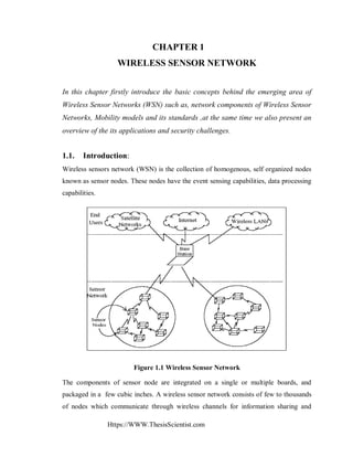
  • 1. Https://WWW.ThesisScientist.com CHAPTER 1 WIRELESS SENSOR NETWORK In this chapter firstly introduce the basic concepts behind the emerging area of Wireless Sensor Networks (WSN) such as, network components of Wireless Sensor Networks, Mobility models and its standards ,at the same time we also present an overview of the its applications and security challenges. 1.1. Introduction: Wireless sensors network (WSN) is the collection of homogenous, self organized nodes known as sensor nodes. These nodes have the event sensing capabilities, data processing capabilities. Figure 1.1 Wireless Sensor Network The components of sensor node are integrated on a single or multiple boards, and packaged in a few cubic inches. A wireless sensor network consists of few to thousands of nodes which communicate through wireless channels for information sharing and
  • 2. Https://WWW.ThesisScientist.com cooperative processing. A user can retrieve information of his/her interest from the wireless sensor network by putting queries and gathering results from the base stations or sink nodes. The base stations in wireless sensor networks behave as an interface between users and the network. Wireless sensor networks can also be considered as a distributed database as the sensor networks can be connected to the Internet, through which global information sharing becomes feasible. Wireless Sensor Networks consist of number of individual nodes that are able to interact with the environment by sensing physical parameter or controlling the physical parameters, these nodes have to collaborate in order to fulfil their tasks as usually, a single node is incapable of doing so and they use wireless communication to enable this collaboration. 1.1.1 Wireless Sensor Network Model: The major components of a typical sensor network are:  Sensor Field: A sensor field is the area in which the all sensors nodes are placed. Figure 1.2 : Wireless Sensor network model  Sensor nodes: Sensor node has capabilities of event sensing, data processing and communication capabilities.  Sink: A sink is a sensor node with the specific task of data receiving, data processing and data storing from the other sensor nodes. They serve to reduce the total number of messages that need to be sent, hence reducing the overall energy requirements of the network. Sinks are also known as data aggregation points.
  • 3. Https://WWW.ThesisScientist.com  Task Manager: The task manager also known as base station is a centralised point of control within the network that extracts information from the network. 1.1.2 Network Components of a Wireless Sensor Node: The main components of a general WSN are the sensor nodes, the sink (base station).  Sensing Unit: Sensors play a very important role in wireless sensor networks by creating a connection between physical world and computation world. Sensor is a hardware device used to measure the change in physical condition of an area of interest and produce response to that change. It converts the analogue data (sensed data from an environment) to digital data and then sends it to the microcontroller for further processing.  A typical wireless sensor node is a micro-electronic node with less than 0.5 Ah and 1.2 V power source. Figure 1.3: Components of a Wireless Sensor Node
  • 4. Https://WWW.ThesisScientist.com  Memory Unit: Memory unit of the sensor node is used to store both the data and program code. For data packets storing from neighbouring (other) nodes Random Only Memory (ROM) is normally used and to storing the program code, flash memory or Electrically Erasable Programmable Read Only Memory (EEPRM) is used.  Power Unit: A sensor node consist a power unit that responsible for computation and transmission and deliver power to all its units. The basic power consumption at node is due to computation and transmission where transmission is the most expensive activity at sensor node in terms of power consumption. Mostly, sensor nodes are battery operated but it can also scavenge energy from the environment through solar cells.  Processing Unit: Processing unit is responsible for data acquisition, processing incoming and outgoing information, implementing and adjusting routing information considering the performance conditions of the transmission. Sensor node has a microcontroller which consist a processing unit, memory, converters (analogue to digital, ATD) timer and Universal Asynchronous Receive and Transmit (UART) interfaces to do the processing tasks. 1.1.3 WSN Communication Architecture: The protocol stack consists of the physical layer, data link layer, network layer, transport layer and application layer. And also consist of power management plane, mobility management plane and task management plane. The main usage of protocol stack are integrating data with networking protocols, communicates power efficiently through the wireless medium. The physical layer is required for carrier frequency generation, frequency selection, signal detection, modulation and data encryption, transmission and receiving mechanisms. The Data Link Layer is required for medium access, error control, multiplexing and de- multiplexing of data streams and data frame detection.
  • 5. Https://WWW.ThesisScientist.com It also ensures reliable point to point and point to multi-hop connections in the network. The MAC layer of data link layer provides the facility of collision detection and use minimal power. The network layer is required for routing the information received from the transport layer i.e. finding the most efficient path for the packet to travel on its way to a destination. The Transport Layer is needed when the sensor network intends to be accessed through the internet. It also helps in maintaining the flow of data whenever the application requires it. The application layer is responsible for presenting all required information to the application and application users and propagating requests from the application layer down to the lower layer. Figure 1.4: Protocol Stack 1.2 Clustering in wireless sensor network: In clustering, the sensor nodes are partitioned into different clusters. Each cluster is managed by a node referred as cluster head (CH) and other nodes are referred as cluster nodes. Cluster nodes do not communicate directly with the sink node. They have to pass the collected data to the cluster head and cluster head received from data from cluster nodes and then aggregate the data and transmits it to the base station .Thus minimizes the energy consumption and number of messages communicated to base station. Also number of active nodes in communication is reduced.
  • 6. Https://WWW.ThesisScientist.com Sensor Node: It is the core component of wireless sensor network. It has the capability of sensing, processing, routing, etc. Cluster Head: The Cluster head (CH) is the master for all nodes in the specific cluster and responsible for different activities carried out in the cluster, such as data aggregation, data transmission to base station, scheduling in the cluster, etc. Base Station: Base station is considered as a main data collection node for the entire sensor network. It is the bridge between the sensor network and the end user. Normally this node is considered as a node with no power constraints. Figure 1.5: Clustered Sensor Network Cluster: It is the organizational unit of the network, created to simplify the communication in the sensor network. Advantages of Clustering:  Scalability for large number of nodes  Reduces communication overhead  Efficient use of resources in WSNs  Transmit aggregated data to the data sink  Reducing number of nodes taking part in transmission  Useful Energy consumption
  • 7. Https://WWW.ThesisScientist.com  1.3. Characteristics of Wireless Sensor Networks Wireless Sensor Networks have some unique characteristics. These are:  Low power consumption: Sensor nodes are small-scale devices with volumes approaching a cubic millimetre in the near future. Such small devices are very limited in the amount of energy they can store or harvest from the environment.  Ability to cope with node failures: Nodes are subject to failures due to depleted batteries or, more generally, due to environmental influences. Limited size and energy also typically means restricted resources (CPU performance, memory, wireless communication bandwidth and range).  Limited Communication Capability: The transmission range of a sensor nodes is varied from tens of meters to hundreds of meters, which is highly depend on the geographical environments and the natural causes. The bandwidth of a sensor node is also very limited. Consequently, how to finish the expected tasks under the constraint of limited communication capability is a challenge issue in Wireless Sensor Networks.  Limited Computing and Storage Capabilities: The computing, processing, and storage capabilities of sensor nodes are very limited. Thus, only some basic data processing and computing tasks can be finished on a node. Meanwhile, the memory and storage space of sensor nodes are also very limited, where some temporary data can be stored.  Dynamic Network: Wireless Sensor Networks are large-scale networks. During the working process of a Wireless Sensor Networks, some nodes may die due to exhaust their energy or damaged by some other causes, and some new nodes may come to join the network. Hence, how to deal with this dynamics for Wireless Sensor Networks and make the network adapt the changes is a challenge issue when design algorithms and protocols for Wireless Sensor Networks  Huge Data Flows: The data produced by the sensor nodes by viewed as data flows. Intuitively, as time goes on, huge data flows are generated by a Wireless Sensor Networks. Among these data flows, there may be a lot of redundant data. Considering the limitations of sensors nodes on computing, communication, and
  • 8. Https://WWW.ThesisScientist.com storage capabilities, how to manage, query, analyze, and utilize these data is another challenge works for researchers. 1.4. Applications of Wireless Sensor Networks: Wireless sensor network can be developed for various types of application based on its data delivery, application type and application objective. Generally WSN application can be classified into following four classes. 1. Commercial and Industrial Applications: a. Monitoring an Industrial Plant: The wireless sensors are used to monitor the state of the physical plant and control device Cost savings can be achieved through inexpensive wireless means. b. Inventory Control: Sensor nodes are used for warehouses products tagging. This will enable the users to track the exact location of the products as well as inventory the stock on hand. Inserting new products can be achieved by attaching the appropriate sensor nodes to the products. If the products are perishable, the senor node can also report the state of the products such as days in storage or temperature. 2. Health Applications a. Gym Workout Performance Monitoring: The gym member users pulse and respiratory rate can be monitored via wireless sensor nodes and transmitted to a personal computer for analysis. The gym club can monitors the exercise behaviour of members and intervene when members need help reaching their goals. b. Monitoring of Human Physiological Data: Sensor nodes can collected the physiological data and stored over a period of time to study human habits and behaviour. Sensor nodes allow greater freedom of movement and allow physicians to either monitor an existing condition. 3. Environmental Applications: a. Soil Condition Monitoring: Sensor nodes can monitor soil temperature and moisture for a given area. The sensor nodes can also be fitted with a variety of chemical and
  • 9. Https://WWW.ThesisScientist.com biological sensors so that the farmers can determine the level of fertilizer. This application is most suited for vineyards as minor changes in the environment can greatly affect the value of the crop and how it is subsequently processed. b. Seismic Activity Detection: Sensor nodes placed in regions for detection of seismic activity such as earthquakes, volcanic eruptions or a tsunami. Timely analysis of such information will enable cities to be evacuated. Sensor nodes placed in regions of seismic activity will enable geologists to monitor and predict the onset of an earthquake, volcanic eruption or a tsunami. 4. Security and Military Applications: A wireless sensor network can be an integral part of military command, intelligence, surveillance, targeting systems, control, computing, and communications. They can be quickly deployed and are fault tolerant, which makes them an ideal sensing technique for reconnaissance and surveillance. a. Monitoring of Force Movement and Inventory: Wireless sensor networks can be used for monitoring of force movement and availability of equipment and ammunition. This will enable the military commander to give order to his forces or equipment to where it is needed most. b. Battlefield Reconnaissance and Surveillance: A wireless sensor network can be used to locate and identify targets for potential attacks or to support an attack by friendly forces Deployed .And wireless sensors networks can also be used in place of guards or sentries 1.5 Motivation Recent research into wireless sensor network (WSN) has attracted great interest because of its advantages like self identification, self diagnostics, reliability, time awareness for co-ordination with other nodes. In WSN nodes in a network communicate with each other via wireless communication. Moreover, the energy required to transmit a message is about twice as great as the energy needed to receive the same message. The route of each message destined to the base station is really crucial in terms network lifetime: e.g., using short routes to the base station that contains nodes with depleted batteries may yield
  • 10. Https://WWW.ThesisScientist.com decreased network lifetime. On the other hand, using a long route composed of many sensor nodes can significantly increase the network delay. But, some requirements for the routing protocols are conflicting. Always selecting the shortest route towards the base station causes the intermediate nodes to deplete faster, this result in a decreased network lifetime. At the same time, always choosing the shortest path might result in lowest energy consumption and lowest network delay. Finally, the routing objectives are tailored by the application; e.g., real-time applications require minimal network delay, while applications performing statistical computations may require maximized network lifetime. Hence, different routing mechanisms have been proposed for different applications. These routing mechanisms primarily differ in terms of routing objectives and routing techniques, where the techniques are mainly influenced by the network characteristics. 1.6. Aims and objectives: The main aim of this research study is to identify the performance challenges for selected routing protocols in wireless sensors and then evaluate the selected routing protocols for a selected application environment (Static and Mobile) against the set of qualitative performance metrics for any protocol. Furthermore the another main objective of this thesis is to identify delivery demand of the communication for the selected application, to compare different routing protocols for these applications and to identify the protocol suitability in the selected application environment on the basis of performance results in order to attain efficient communication and save network resources. The particular goals of this thesis work are to:  Develop and design a simulation model and scenarios.  Perform a simulation with different metrics and different scenarios.  Analysis of the results in static and mobile environment.  Comparative study has been done on the basis of simulation results.  Deriving a conclusion on basis of performance evaluation. 1.7. Simulation Tool
  • 11. Https://WWW.ThesisScientist.com In our dissertation work we are using the Optimized Network Engineering Tool (OPNET v16.0) software for simulating selected routing protocols. OPNET is a network simulator. Figure1.7: Flow chart of OPNET It provides multiple solutions for managing networks and applications e.g. network operation, planning, research and development (R&D), network engineering and performance management. OPNET 16.0 is designed for modelling communication devices, technologies, and protocols and to simulate the performance of these technologies. It allows the user to design and study the network communication devices, protocols, individual applications and also simulate the performance of routing protocol. It supports many wireless technologies and standards such as, IEEE 2002.11, IEEE 2002.15.1, IEEE 2002.16, IEEE 2002.20 and satellite networks. OPNET IT Guru Academic Edition is available for free to the academic research and teaching community. It provides a virtual network environment that models the behaviour of an entire network including its switches, routers, servers, protocols and individual application. The main merits of OPNET are that it is much easier to use, very user friendly graphical user interface and provide good quality of documentation. 1.8. RESEARCH METHODOLOGY
  • 12. Https://WWW.ThesisScientist.com Research methodology defines how the development work should be carried out in the form of research activity. Research methodology can be understand as a tool that is used to investigate some area, for which data is collected, analyzed and on the basis of the analysis conclusions are drawn. There are three types of research i.e. quantitative, qualitative and mixed approach as defined in. 1. Quantitative Approach This approach is carried out by investigating the problem by means of collecting data, experiments and simulation which gives some results, these results are analyzed and decisions are made on their basis. This approach is used when the researchers‟ want verify the theories they proposed, or observe the information in greater detail. 2. Qualitative Approach This approach is usually involves the knowledge claims. These claims are based on a participatory as well as / or constructive perspectives. This approach follows the strategies such as ethnographies, phenomenology and grounded theories. When the researcher wants to study the context or focusing on single phenomenon or concepts, they used qualitative approach to achieve their desired goals. 3. Mixed Approach Mixed approach glue together both quantitative and qualitative approaches. This approach is followed when the researchers wants to base their knowledge claims on matter of fact grounds. Mixed approach has the ability to produce more complete knowledge necessary to put a theory and practice as it combined both quantitative and qualitative approaches. 4. Author’s Approach Author‟s approach towards the thesis is quantitative. This approach starts by studying the elated literature specific to security issues in MANETs. Literature review is followed by simulation modeling. The results are gathered and analyzed and conclusions are drawn on the basis of the results obtained from simulation. 5. Research Design The author divided the whole research thesis into four stages. 1) Problem Identification and Selection.
  • 13. Https://WWW.ThesisScientist.com 2) Literature study. 3) Building simulation. 4) Result analysis. Figure 1.8: Research Methodology 1) Problem Identification and Selection The most important phase, where it is important to select the proper problem area. Different areas are studied with in mind about the interest of authors. Most of the time is given to this phase to select the hot issue. The authors selected MANET as the area of interest and within MANET the focus was given to the security issues. 2) Literature Study Once the problem was identified the second phase is to review the state of the art. It is important to understand the basic and expertise regarding MANETs and the security issues involved in MANETs. Literature study is conducted to develop a solid background for the research. Different simulation tools and their functionality are studied.
  • 14. Https://WWW.ThesisScientist.com 3) Building Simulation The knowledge background developed in the literature phase is put together to develop and build simulation. Different scenarios are developed according to the requirements of the problems and are simulated. 4) Result Analysis The last stage and important and most of the time is given to this stage. Results obtained from simulation are analyzed carefully and on the basis of analysis, conclusions are drawn.
  • 15. Https://WWW.ThesisScientist.com Chapter 2 LITERATURE REVIEW In this chapter we have studied the various related work on Wireless Sensor Networks (WSNs) such as its routing protocols, its application classes its and its network simulator of Wireless Sensor Networks. By conducting literature survey, we studied different research articles, papers including books to identify factors which highly influence the routing protocols and affect their performance. 2.1 Related Work: Sonam Palden.et al; (2012): In this paper authors proposed a novel energy efficient routing protocol. The proposed protocol is hierarchical and cluster based. In this protocol, the Base Station selects the Cluster Heads (CH). The selection procedure is carried out in two stages. In the first stage, all candidate nodes for becoming CH are listed, based on the parameters like relative distance of the candidate node from the Base Station, remaining energy level, probable number of neighboring sensor nodes the candidate node can have, and the number of times the candidate node has already become the Cluster Head. The Cluster Head generates two schedules for the cluster members namely Sleep and TDMA based Transmit. The data transmission inside the cluster and from the Cluster Head tothe Base Station takes place in a multi-hop fashion. They compared the performance of the proposed protocol with the LEACH through simulation experiments. and observation is that the proposed protocol outperforms LEACH under all circumstances considered during the simulation. As a future scope they state that, the protocol can be enhanced for dealing with mobility of nodes. Even effort can be made to decide the number of clusters dynamically and this may give better scalability to the protocol for dealing with very large wireless sensor networks. P. Kamalakkannan.et al; [2013]: In this paper, they proposed an enhanced algorithm for Low Energy Adaptive Clustering Hierarchy–Mobile (LEACH-M)protocol called ECBR-MWSN which is Enhanced Cluster Based Routing Protocol for Mobile Nodes in Wireless Sensor Network. ECBR-MWSN protocol selects the CHs using the parameters
  • 16. Https://WWW.ThesisScientist.com of highest residual energy, lowest Mobility and least Distance from the Base Station. The Base Station periodically runs the proposed algorithm to select new CHs after a certain period of time. It is aimed to prolonging the lifetime of the sensor networks by balancing the energy consumption of the nodes. The experiments were performed to evaluate the performance of the proposed protocol in terms of four factors like Average Energy Consumption, Packet Delivery Ratio, Throughput, Routing Overhead and Average end to end Delay. The simulations results indicates that the proposed clustering approach is more energy efficient and hence effective in prolonging the network life time compared to LEACH-M and LEACH-ME. They also suggest in future scope that the algorithms and techniques implemented in the proposed protocol will be optimized in order to minimize energy and routing related packets, which in turn lead to reduced routing overhead. Then to find the energy consumption while delivery of packets under non-uniform transmission situations. And also the proposed protocol will improve the performance to decrease the delay. Particularly for reaching the optimal solution for mobile sensor networks is an open issue. Pallavi Jindal. et al; (2013):In this paper authors shows the various routing techniques like LEACH, WLEACH, LEACH-CC, GAF, CODE. They show the comparison between LEACH, WLEACH and LEACH-CC. Their survey shows the limitation of basic leach. Leach use TDMA or CDMA Mac to share channel. The goal of LEACH is to lower the energy consumption required to create and maintain clusters in order to improve the life time of a wireless sensor network. LEACH is a hierarchical protocol in which most nodes transmit to cluster heads, and the cluster heads aggregate and compress the data and forward it to the base station (sink). Each node uses a stochastic algorithm at each round to determine whether it will become a cluster head in this round. LEACH assumes that each node has a radio powerful enough to directly reach the base station or the nearest cluster head, but that using this radio at full power all the time would waste energy. By data-fusion and energy-equilibrium, LEACH can extend the life of network .But there are some disadvantage of leach that are: first it uses random number to decide a node whether becomes a cluster-head node, so when a low-energy node becomes cluster-head node, it will die immediately. Secondly, LEACH doesn‟t care the neighbor nodes when makes cluster head nodes, so when some nodes are far from its cluster-head node in long
  • 17. Https://WWW.ThesisScientist.com time, they will die immediately too. Finally, every node uses single-jump routing to transmit data, which makes that commutation between nodes too costly. L.I. Jian. et al; (2013):in their paper they aim at the node characteristic of uneven distribution in the real environment the improved algorithm combines the advantages of EUUC algorithm and PEGASIS algorithm. The new improved algorithm improves uneven energy consumption of the cluster head nodes under EUUC algorithm, also reduces the complexity of clustering signaling, as well as takes real-time problems into consideration. By calculating dispersion coefficient of the cluster to determine the communication topology within each cluster and by using multi-objective particle swarm optimization to optimize cluster head routing. The simulation results of the algorithm shows that the improved algorithm is more suitable for large-scale wireless sensor networks, and makes overall network performance more effective. But improved algorithm is to measure distance based on the signal intensity. In real application, the signal intensity is to being effected by outside environment. R. Balasubramaniyan et al; (2013):In the paper authors consider the study that in WMASNs, the number of control packets for flooding increases exponentially with the number of nodes. The CBRP (Cluster-Based Routing Protocol)methods were proposed to solve the problem of exponential increase. The CBRP methods have been widely used to achieve efficient management and extension of distributed nodes. Well-known CBRP methods include LCA (Linked Clustered Algorithm), LID (Lowest-ID), LCC (Least Cluster Change),MCC (Maximum Connectivity) and RCC (Random Competition Clustering) . These existing algorithms have clustering criteria for selecting cluster heads and are based on the minimum cluster overlap method in the formation of clusters. These algorithms, however, cannot guarantee stability due to the ambiguity in the selection of cluster heads. Thus, several clustering algorithms were proposed in WMASNs to improve performance and reduce overhead. Selecting the cluster head is based on the mobility of nodes in, and on the mobility of nodes and power capacity in. These algorithms have the advantage of clear selection of the cluster head, but they have the problem of requiring correct information for the attributes and relationships of nodes. Though many clustering algorithms are proposed, few algorithms are dedicated for wireless mobile ad hoc networks.
  • 18. Https://WWW.ThesisScientist.com Ali Norouzi.et al;(2013): In this paper authors made an elaborate study on the routing method featured with optimum energy consumption in wireless sensor networks. Some of routing protocols with high energy efficiency (LEACH, Director Diffusion, Gossiping, PEGASIS, and EESR) were examined. Authors have also view the strategies of the protocol for WSNs such as data aggregation and clustering, routing, different node role assignments, and data-center methods. The routing protocols were compared regarding variety of metrics influencing requirements of the specific application .The result of their paper in which the comparison showed that Gossiping consumes a medium amount of energy and best performance was obtained by PEGASIS and LEACH. Franscisco j. Martinez et al; (2009): In this paper authors present a survey and comparative study of several publicly available network simulators, mobility generators and Wireless sensor networks simulators. In their work , the network simulators like NS- 2, SNS, GloMoSim, SWANS, and QualNet briefly described by authors. In this paper authors also present comparative study of various mobility generator like SUMO, MOVE FreeSim, CityMob, STRAW, and Netstream. In their work authors conclude that SUMO, STRAW and MOVE have good traffic model support and also have some good features but these are the best. Finally the authors present briefly introduction of Wireless sensor networks simulators such as Trans, MobiREAL, GrooveNet, NCTUns. According to the authors survey GrooveNet and NCTUns are more frequently used for Wireless sensor networks simulations than simulation tools. Bhardwaj P. K et al; (2012): In this paper authors analyze performance of two routing protocols AODV and OLSR by using OPNET Modelar 14.5.In their work ,authors create a network scenario of 50 nodes with the comparison of network load media access delay and throughput to examine the AODV and OLSR routing protocols with simulation parameters like 800*800 m campus area , 50 nodes and 20 minutes simulation time .According to the authors simulation result OLSR routing protocol shows low media access delay and low network load in comparison of AODV , with the overall performance OLSR is better than AODV but it is not necessary that OLSR is always better than AODV. Moravejosharieh A. et al; (2013):Here authors, reveals the performance analysis of reactive routing protocols AODV, AOMDV and DSR. In their work, authors performed
  • 19. Https://WWW.ThesisScientist.com comparison with proactive routing protocol DSDV. In this paper authors used NS-2.34 simulation tool for simulation purpose with taken various parameters such as 200 second simulation time , 10*1000 m simulation area and 100 bytes packet size, by using performance metrics such as packet delivery ratio, average packet loss ratio and average end to end delay of packets are investigated on the basis of node velocity and node density . According to the authors simulation result, DSDV routing protocol shows the worst packet delivery ratio and AOMDV and AODV have highest average end to end delays. Siva D. Muruganathan. et al; (2010):here authors have made a comparison between the average query response time of the Two-level Hierarchical Clustering based Hybrid- routing Protocol (THCHP) and Adaptive Periodic Threshold-sensitive Energy Efficient sensor Network (APTEEN)Protocol, and the result shows that THCHP is better suited than APTEEN for delay sensitive WSN applications such as forest fire detection. APTEEN utilizes adaptive threshold values and a periodic update interval parameter to switch between proactive and reactive modes of data routing where as THCHP, an alternative hybrid routing protocol. Waghmare et al; (2008):in this paper authors try to make best use of GRPC channels by proposing a cluster based multi channel communication scheme. In this scheme authors assumed that each sensors node is equipped with two GRPC transceiver that can work on two different channel simultaneously. In their work they divide time in to periods that can be repeated every T millisecond. And each period is further divide into sub periods for exchange data. Mahmud et al; (2008):Here, authors proposed a hybrid media access technique for cluster based wireless sensors networks ,this technique is based on the scheduled based approach such as TDMA for intra cluster based communications and management , and contention based approach for the inter cluster based communications and management. In this scheme authors used a control channel for delivering the safety and non safety application related messages to the nearby clusters. Wan-Li Zhao. et al;(2010): in this paper authors have discussed the routing algorithm like Leach a clustering routing protocol which was first proposed in wireless sensor networks. Cluster head in LEACH can be randomly selected to average the power
  • 20. Https://WWW.ThesisScientist.com consumption in the whole network, yet the cluster head selection ignores such indicators as the residual energy of the nodes and the number of neighboring nodes. As a result, a node tends to act as a cluster head node for too long before it gets ineffective or there is no cluster head node to manage an area for a long time with slim chances of data collection. Even worse, from the perspective of the whole network, cluster heads are not optimized. Secondly, in HEED algorithm there are two parameters as the main references in cluster head selection. The major parameter depending on the residual energy of the node is used to randomly select the set of the initial cluster headed nodes. The node with more residual energy will be a cluster head in large probability. Paul J.M. Havinga. et al; (2013): in this paper authors made the study of basic clustering algorithm Leach. A comparison is made between Leach and Leach. In this paper they propose REC+, a Reliable and Energy-efficient Chain-cluster based routing protocol, which aims to achieve the maximum reliability in a multi-hop network by finding the best place for the Cluster Head (CH) and the proper shape/size of the clusters without the need of using any error controlling approaches that can be quite expensive in terms of computation and communication overhead. Most importantly, REC+ relaxes some strong assumptions that other cluster-based routing algorithms rely on, which make them inapplicable for real WSNs. Simulation results show that REC+ outperforms a number of other approaches in terms of delay, energy, delay*energy and lifetime. Compared with existing approaches that reform clusters in each round, REC+ starts to change the clusters hopes when the energy goes below a threshold or end to end reliability changes significantly. In the ongoing work, authors will work on making this centralized cluster-chain routing approach autonomous and distributed. Akyildiz.I.F. et al;(2002):In this paper authors present a communication architecture for wireless sensor networks and proceed to survey the current research pertaining to all layers of the protocol stack: Physical, Data Link, Network, Transport and Application layers. A wireless sensor network is deal as being composed of a large number of nodes which are deployed dense lyin close proximity to the phenomenon to be monitored. Each of these nodes collects data and its purpose is to route this information back to a sink. The network must possess self-organizing capabilities since the positions of individual nodes are not predetermined. The authors point out that none of the studies surveyed has a fully
  • 21. Https://WWW.ThesisScientist.com integrated view of all the factors driving the design of sensor networks and proceeds to present its own communication architecture and design factors to be used as a guideline and as a tool to compare various protocols.
  • 22. Https://WWW.ThesisScientist.com Chapter 3 BACKGROUND OF WSN 3.1 Classification of Routing protocols in WSN: Routing protocol of WSN can be categorized according to the nature of wireless sensor network and its architecture. Wireless sensors network can be classified in to two broad categories, network architecture based routing protocols and route selection based routing protocols. 3.1.1 Architecture Based Routing Protocols: In the WSN routing protocols can also divided according to the structure of network.Protocols included into this category are further divided into three subcategories according to their functionalities. These protocols are:  Flat-based routing  Hierarchical-based routing  Location-based routing 3.1.2 Route Selection Based Routing Protocols: This classification of protocol is based on how the source node finds a route to a destination node and can be further classified in to two categories. Proactive Routing Protocols:.These types of protocols are table based because they maintain table of connected nodes to transmit data from one node to another and each node share its table withanother node. Reactive Routing Protocols: These type of routing protocols is also known as On Demand routing protocols because it establish a route from source to destination whenever a node has something to send thus reducing burden on network. 3.2 Architecture Based Routing Protocols:
  • 23. Https://WWW.ThesisScientist.com In the WSN routing protocols can also divided according to the structure of network.Protocols included into this category are further divided into three subcategories according to their functionalities. These protocols are:  Flat-based routing  Hierarchical-based routing  Location-based routing 3.2.1 Flat-Based Routing: Flat-based routing is needed when huge amount of sensor nodes are required, where every node plays same role. In this type of routing the number of sensor nodes is very large therefore it is not possible to assign a particular Id to each and every node. This leads to data-centric routing approach in which Base station sends query to a group of particular nodes in a region and waits for response. Examples of Flat-based routing protocols are:  Energy Aware Routing (EAR)  Directed Diffusion (DD)  Sequential Assignment Routing (SAR)  Minimum Cost Forwarding Algorithm (MCFA)  Sensor Protocols for Information via Negotiation (SPIN)  Active Query forwarding In sensor network (ACQUIRE) Directed Diffusion (DD):Data aggregation model for a wireless sensor network known as directed diffusion routing protocol. The main idea of Data aggregation model is to dispose of unnecessary network operations through combining the data coming from different sources of route, eliminating redundancy, minimizing the number of transmissions. Directed diffusion is a data-centric and application aware model in the sense that all data generated by sensor nodes is named by attribute value pairs such as name of objects, interval, duration, geographic location etc. A base station may request data by broadcasting interests and each node receiving the interest can store in the cache the interest. The interests in the caches are compared with the received data with the values of the interest. This enables diffusion to achieve energy savings later by selecting empirically good paths. Each sensor node that receives the interest establishes a gradient
  • 24. Https://WWW.ThesisScientist.com toward the sensor node from which it received the interest. This process continues until gradients are built from the source back to the base station. Figure 5 shows an example of the workings of directed diffusion. Figure 3.1: Simplified Schematic for Directed Diffusion Directed diffusion routing protocol different from SPIN routing protocol in two aspects. The first being that directed diffusion routing protocol issues data queries on the basis of demand as the base station sends the queries to the sensor nodes. In SPIN routing protocol, nodes advertise the presence of data allowing the interested node to query that data. The second is that all communication in directed diffusion routing protocol is neighbor to neighbor with each node having the capability to perform data aggregation and caching. There is no need to maintain a global network topology, unlike SPIN routing protocol. However, directed diffusion may not be applied to applications that require continuous data delivery such as habitat monitoring since it is a query driven system. SPIN: Sensor Protocols for Information via Negotiation (SPIN) was designed to improve classic flooding protocols. It fit under data delivery model in which the nodes sense data and disseminate the data throughout the network by means of negotiation. In the SPIN routing protocol nodes use three types of messages for communication:
  • 25. Https://WWW.ThesisScientist.com  ADV messages -When a node has new data to share; it can advertise this using ADV message containing Metadata.  REQ messages - When it needs to receive actual data node sends an REQ.  DATA messages -DATA messages consist of actual data. The SPIN family Protocol is made up of four protocols, SPIN-PP, SPIN-EC, SPIN-RL and SPIN-BC. Figure 3.2: SPIN Protocol. In above figure. (a) Node A starts by advertising its data to node B (b) Node B responds by sending a request to node A. (c) After receiving the requested data. (d) Node B then sends out advertisements to its neighbours. (e) Who in turn send request s back to B (e-f). 3.2.2 Hierarchical-Based Routing: Hierarchical-based routing is used when network scalability and efficient communication is needed. It is also called cluster based routing. Hierarchical-based routing is energy efficient method in which high energy nodes are randomly selected for processing and
  • 26. Https://WWW.ThesisScientist.com sending data while low energy nodes are used for sensing and send information to the cluster heads. This property of hierarchical-based routing contributes greatly to the network scalability, lifetime and minimum energy. Examples of hierarchical-based routing protocols are;  Hierarchical Power-Active Routing (HPAR)  Threshold sensitive energy efficient sensor network protocol (TEEN)  Power efficient gathering in sensor information systems  Minimum energy communication network (MECN) TEEN and APTEEN: Threshold sensitive Energy Efficient sensor Network protocol (TEEN) is a hierarchical protocol designed to be responsive to sudden changes in the sensed attributes such as temperature. TEEN routing protocol using a hierarchical approach along with the use of a data-centric mechanism. The sensor network architecture is based on a hierarchical grouping where closer nodes form clusters and this process goes on the second level until base station (sink) is reached. The model is shown in Figure given below. After the clusters are formed, the cluster head broadcasts two thresholds to the nodes, one is the hard threshold and another is the soft threshold. The hard threshold allows the nodes to transmit only when the sensed attribute is in the range of interest, thus reducing the number of transmissions significantly. Once a node senses a value at or beyond the hard threshold, it transmits data only when the value of that attribute changes by an amount equal to or greater than the soft threshold. As a consequence, soft threshold will further reduce the number of transmissions if there is little or no change in the value of sensed attribute. One can adjust both hard and soft threshold values in order to control the number of packet transmissions. However, TEEN is not good for applications where periodic reports are needed since the user may not get any data at all if the thresholds are not reached. The Adaptive Threshold sensitive Energy Efficient sensor Network protocol (APTEEN) is an extension to TEEN routing protocol. The architecture of APTEEN routing protocol is same as in TEEN routing protocol. When the base station forms the clusters, the cluster heads broadcast the attributes, the threshold values, and the transmission schedule to all nodes. Cluster heads also perform data aggregation in order to save energy.
  • 27. Https://WWW.ThesisScientist.com Figure 3.3: Hierarchical Clustering in TEEN and APTEEN APTEEN routing protocol supports three different query types: historical queries, past data values queries; one-time queries, to take a snapshot view of the network; and persistent to monitor an event for a period of time. Simulation of TEEN routing protocol and APTEEN routing protocol has shown them to outperform LEACH routing protocol. The experiments have demonstrated that APTEEN‟s routing protocol performance is between LEACH routing protocol and TEEN routing protocol in terms of energy dissipation and network lifetime. TEEN routing protocol gives the best performance since it decreases the number of transmissions. The main drawbacks of the two approaches are the overhead and complexity of forming clusters in multiple levels, implementing threshold-based functions and dealing with attribute-based naming of queries. 3.2.3 Location-Based Routing In the location based routing, sensor nodes are scattered randomly in an area of interest. They are located mostly by using of Global position system. The distance between the sensor nodes is estimated by the signal strength received from those nodes and
  • 28. Https://WWW.ThesisScientist.com coordinates are calculated by exchanging information between neighbouring nodes. Location-based routing networks are; Sequential assignment routing (SAR)  Ad-hoc positioning system (APS)  Geographic adaptive fidelity (GAP)  Greedy other adaptive face routing (GOAFR)  Geographic and energy aware routing (GEAR)  Geographic distance routing (GEDIR) Geographic Adaptive Fidelity (GAF): Geographic Adaptive Fidelity is an energy- aware location based routing algorithm designed for mobile ad-hoc networks but has been applied to wireless sensor networks. Geographic Adaptive Fidelity conserving energy by switching off redundant sensors nodes. In this routing protocol whole network is divided into number of fixed zones and a virtual grid is formed for the covered area. Each node uses its GPS-indicated location to associate itself with a point in the virtual grid. Nodes associated with the same point on the grid are considered equivalent in terms of packet routing costs. Nodes within a zone collaborate by electing one node to represent the zone for a time period while the rest of the nodes sleep. A sample situation is taken from illustrated below. In the figure, node 1 can reach any of nodes, 2, 3 or 4. Nodes 2, 3 and 4 can reach node 5.Therefore, nodes 2, 3 and 4 are equivalent and two of them can sleep. Figure 3.4 Example of Virtual Grid in GAF Nodes rotate the active and sleep states so that the load to each node is balanced. It was noted that as the number of nodes increase, so would the lifetime of the network. There
  • 29. Https://WWW.ThesisScientist.com are three states in the defined in GAF. These states are: discovery for determining the neighbours in the grid, active reflecting the participation in the routing and sleep when the radio is turned off. The state transitions taken from are depicted below. Figure 3.5 State Transitions in GAF GAF is a location based routing protocol but may also be considered a hierarchical based protocol where clusters are based on geographic location. In a particular grid, a representative node acts as a leader node to transmit data to other nodes. The leader node, however, does not do data aggregation or fusion as in hierarchical protocol discussed earlier. GEAR: In the GEAR routing protocol, each node keeps an estimated cost and a learning cost of reaching the destination through neighbors. Figure 3.6 Geographic Forwarding in GEAR
  • 30. Https://WWW.ThesisScientist.com The estimated cost is a combination of residual energy and distance to destination. Hole occurs when a node does not have any closer neighbors to the target. If there are no holes, the estimated cost equal to the estimated cost is equal to the learned cost. The learned cost is propagated one hop back every time a packet reaches the destination so that route set up for next packet will be adjusted. 3.3 Route Selection Base Classification of Routing Protocols: This classification of protocol is based on how the source node finds a route to a destination node and can be further classified in to two categories. 3.3.1: Proactive Routing Protocols: Figure 3.7: Proactive routing protocols routing scheme These types of protocols are table based because they maintain table of connected nodes to transmit data from one node to another and each node share its table with another node. Different types of proactive routing protocols are Destination Sequence Distance Vector Routing (DSDV), Optimized link state routing (OLSR) and Fisheye State Routing.
  • 31. Https://WWW.ThesisScientist.com A. Optimized Link State Routing Protocol (OLSR): The Optimized Link State Routing (OLSR) protocol is described in RFC3626 [7]. OLSR is proactive routing protocol that is also known as table driven protocol by the fact that it updates its routing tables. OLSR has also three types of control messages which are describe bellow. Hello: This control message is transmitted for sensing the neighbor and for Multi Point Distribution Relays (MPR) calculation. Topology Control (TC): These are link state signaling that is performed by OLSR. MPRs are used to optimize theses messaging. Multiple Interface Declaration (MID): MID messages contains the list of all IP addresses used by any node in the network. All the nodes running OLSR transmit these messages on more than one interface. OLSR Working Multi Point Relaying (MPR) OLSR diffuses the network topology information by flooding the packets throughout the network. The flooding is done in such way that each node that received the packets retransmits the received packets. These packets contain a sequence number so as to avoid loops. The receiver nodes register this sequence number making sure that the packet is retransmitted once. The basic concept of MPR is to reduce the duplication or loops of retransmissions of the packets. Fig.1.5 Flooding Packets using MPR Only MPR nodes broadcast route packets. The nodes within the network keep a list of MPR nodes. MPR nodes are selected with in the vicinity of the source node. The selection of MPR is based on HELLO message sent between the neighbor nodes. The
  • 32. Https://WWW.ThesisScientist.com selection of MPR is such that, a path exist to each of its 2 hop neighbors through MPR node. Routes are established, once it is done the source node that wants to initiate transmission can start sending data. The whole process can be understood by looking into the Fig.1.6 below. The nodes shown in the figure are neighbors. “A” sends a HELLO message to the neighbor node “B”. When node B receives this message, the link is asymmetric. The same is the case when B send HELLO message to A. When there is two way communications between both of the nodes we call the link as symmetric link. HELLO message has all the information about the neighbors. MPR node broadcast topology control (TC) message, along with link status information at a predetermined TC interval. Fig: 1.6 Hello Message Exchange B. Destination Sequence Distance Vector Routing (DSDV): Destination Sequence Distance Vector Routing (DSDV)is a table driven routing protocol based on the Bellman-Ford algorithm. In this type of routing protocol every node in the network share packet with its entire neighbor. And packet contain information such as node‟s IP address, last known sequence number, hop count. Whenever there is topology change in network each node advertises its routing status after a fixed time or immediately. Working of Destination Sequence Distance Vector Routing (DSDV): The main objective of DSDV routing protocol is to avoiding loop formation and maintains its simplicity. In DSDV whenever any node want to transmitted a packet or information to the destination node, it using the routing table. Routing tables are maintained by each node in the network, each node routing table maintains some information like destination address, number of hops required to reach the destination and sequence number. Thus the routing table consist of following entries <destination, distance, next hop>.
  • 33. Https://WWW.ThesisScientist.com Figure 3.8: Example of Destination Sequence Distance Vector Routing operation. Whenever any node want to sending a message to other node than it adds a sequence number in the routing entries, the sequence number indicates the newness of the information to the routing table. In DSDV routing protocol routes with the latest sequence number are always preferred for forwarding a message to one node to other. If one or more source have same sequence number and sending a message to the same destination then in this case route with lower distance is preferred. Routing in DSDV: In the Table 2.1 represent a structure of routing table entries which is maintained at Destination (D) and the table 2.2 represent the exchanged messages. Table 3.1 Routing table entries maintained at Destination (D). Destination Next Hop Distance Sequence No. A B C D S A C C D A 1 2 1 0 2 6 6 6 6 6 In the starting, node D sends a message that broadcast its routing entries to its neighboring nodes , A and C. The neighboring nodes update their routing tables entries and then broadcast a new packet for informing to the all neighboring nodes that the destination node D will be reach through them. Next, the node A receives a message from node B, which announces that the node D at distance 2 and sequence number 6. As
  • 34. Https://WWW.ThesisScientist.com node A already has a routing entry for the destination node D with the same sequence number 6 and lower distance i.e. 1, it will ignore this message because both information are equally fresh, but the first provides a shorter route. Table 3.2 Exchanged message by D Destination Distance Sequence No. A B C D S 1 2 1 0 2 6 6 6 6 6 Therefore, finally, node S can set up a route to node D with distance 2 and node A as the next hop. For example if a node D moves and is no longer in the neighborhood of A and C, but is in neighborhood of S as given in figure 3.9. Figure 3.9 : Node D moves and the network topology changes accordingly. C. Ad hoc On Demand Distance Vector (AODV): Ad hoc On Demand Distance Vector(AODV)is an pure reactive routing protocol which is capable of both unicasting and multicasting. In Ad hoc On Demand Distance Vector (AODV), like all reactive protocols, it works on demand basis when it is required by the nodes within the network. When source node has to send some data to destination node then initially it propagates Route Request (RREQ) message which is forwarded by intermediate nodes until destination is reached. A route reply message is unicasted back
  • 35. Https://WWW.ThesisScientist.com to the source node if the receiver is either the node using the requested address, or ithas a valid route to the requested address that is shown is figure 2.10. (a) (b) Figure 3.10:AODV route discovery process. (a) Propagation of the RREQ. (b) Path of the RREP to the source. Working of Ad Hoc On Demand Distance Vector Routing (AODV):The Ad hoc On- Demand Distance Vector (AODV) allows the communication between two nodes via intermediated nodes, if those two nodes are not within the range of each other. To establish a route between source to the destination, AODV using route discovery phase, along which Route Request message (RREQ) messages are broadcasted to all its neighboring nodes. This phase makes sure that these routes do not forms any loops and find only the shortest possible route to the destination node. It also uses destination sequence number for each route entry, that ensures the loop free route, this is the one of the main benefit of AODV routing protocol. For example if two different sources sends two different request to a same destination node, then a requesting node selects the one with greatest sequence number. In the route discovery phase several control messages are defined in AODV. Different control messages are defined as follows. RREQ (Route Request):When any node wants to communicate with other node then it broadcast route request message(RREQ) to its neighboring nodes. This message is
  • 36. Https://WWW.ThesisScientist.com forwarded by all intermediate nodes until destination is reached. The route request messages (RREQ) contains the some information such as RREQ id or broadcast id, source and destination IP address, source and destination sequence number and a counter. RREP(Route Reply):When any intermediate nodes received Route Request (RREQ) message then it unicast the route reply message (RREP) to source node either it is valid destination or it has path to destination and reverse path is constructed between source and destination. Each route reply message (RREP) packet consist of some information such as hop count, destination sequence number, source and destination IP address. RERR (Route Error): Whenever there is any link failure arises in the routing process then route error message (RERR) is used for link failure notifications. The route error message RERR) consist of some information such as Unreachable Destination node IP Address, Unreachable Destination node Sequence Number. AODV Route Table Management: In AODV, Routing table management is required to avoid those entities of nodes that do not exist or having invalid route from source to destination. The need for routing table management is important to make communication loop free. It consists of following characteristics to maintain the route table for each node. •Destination IP address • Total number of hops to the destination • Destination sequence numbers • Number of active neighbors • Route expiration time AODV Route Maintenance: In AODV ,when any node in the network detects that a route is not valid anymore for communication it delete all the related entries from the routing table .And it sends the Route reply message(RREP) to all current active neighboring nodes to inform that the route is not valid anymore for communication purpose. 3.3.2: Reactive Routing Protocols: These type of routing protocols is also known as On Demand routing protocols
  • 37. Https://WWW.ThesisScientist.com Figure 3.12 : Reactive routing protocols routing scheme because it establish a route from source to destination whenever a node has something to send thus reducing burden on network. Reactive routing have route discovery phase where network is flooded in search of destination that shown in figure 2.12. There are different types of Reactive routing protocols like AODV, DSR, TORA. A. Dynamic Source Routing (DSR): One of the reactive protocols is dynamic source routing protocol. In this protocol it make possible for all the nodes to find a route to a destination in a multiple network hops dynamically. DSR routing protocol minimizes the overall network bandwidth overhead .And DSR also tries to conserve battery power as well as avoidance of routing updates that are large enough. However there is a support from the MAC layer that informs the routing protocol of any failure in nodes in DSR. Some properties of Dynamic source routing are:  In DSR the intermediate nodes do not save the up-to date routing information, thus DSR takes the advantage of source routing.  The network bandwidth is reduced because there are not periodic message advertisements.
  • 38. Https://WWW.ThesisScientist.com  By not sending or receiving advertisements the battery power is also reserved by DSR.  DSR scans for information in packets that are received and learns about the routes. i) Route Discovery DSR routing protocol all the known routes are stored in the cache. When a node wants to send data to another node, it first broadcasts an RREQ (Route request). This RREQ (Route request) is received by other nodes and as they receive it they start searching their cache for any available route to the destination node. In case on any unavailable routes this RREQ (Route request) is forwarded while the address of the current node is being recorded in the hop sequence. The RREQ (Route request) propagates in the network until the availability of a route to the destination or the availability of the destination itself. When this happens an RREP (Route reply) is generated and unicasted to the source node. The contents of this RREP (Route reply) packet are the sequence of hops in the network for reaching the destination node. Figure 3.13: DSR route discovery target node ii) Route Maintenance when any node in the network detects that a route is not valid anymore for communication it delete all the related entries from the routing table .And it sends the Route reply message(RREP) to all current active neighboring nodes to inform that the route is not valid anymore for communication purpose.
  • 39. Https://WWW.ThesisScientist.com Figure 3.14: DSR maintenance for error route. 3.4 Simulation and Simulation Tools: Simulation is three phase process which includes the designing of a model for theoretical or actual system followed by the process of executing this model on a digital computer and finally the analysis of the output from the execution. Simulation is learning by doing which means that to understand/ learn about any system, first we have to design a model for it and execute it. To understand a simulation model first we need to know about system and model. System is an entity which exists and operates in time while model is the representation of that system at particular point in time and space. This simplified representation of system used for it better understating. In wireless sensor network there are many simulation tools are used for simulation purpose describe as below: A. NCTUns: NCTUns (National Chiao Tung University Network Simulation) is a simulator that combines both traffic and network simulator in to a single module that built using C++ programming language and support high level of GUI support. It is a highly extensible and robust network simulator in no need to be concerned about the code complexity. Features:  It can simulate many standards such as IEEE 802.11a, IEEE 802.11b, IEEE 802.11e,IEEE 802.16d, IEEE802.11g and IEEE 802.11.  It supports large number of nodes.  It includes directional, bidirectional and omni directional commutation.
  • 40. Https://WWW.ThesisScientist.com B. NS-2(Network Simulator): Network Simulator (Version 2), called as the NS-2, is simply an event driven , open source ,portable simulation tool that used in studying the dynamic nature of communication networks. Users is feeding the name of a TCL simulation script as an input argument of an NS-2 executable command ns. NS-2 consists of two key languages one is the C++ and second is the Object-oriented Tool Command Language (OTCL). In NS-2 C++ defines the internal mechanism (backend) of the simulation objects, and OTCL defines external simulation environment (i.e., a frontend)for assembling and configuring the objects. After simulation, NS-2 gives simulation outputs either in form of text- based or animation-based. C. OPNET (Optimized network engineering tool): OPNET is a commercial network simulator environment used for simulations of both wired and wireless networks. It allows the user to design and study the network communication devices, protocols and also simulate the performance of routing protocol. This simulator follows the object oriented modelling approach. It supports many wireless technologies and standards such as,IEEE 802.11 , IEEE 802.15.1, IEEE 802.16, IEEE 802.20 and satellite networks. D. QualNet (Quality Networking): QualNet is a highly scalable , fastest simulator for large heterogeneous network It supports the wired and wireless network protocol. QualNet execute any type of scenario 5 to 10 times faster than other simulators. It is highly scalable and simulate up to 50,000 mobile nodes. And this simulator is designed as a powerful Graphical User Interface (GUI) for custom code development. one of the main advantage of QualNet is that it supports Windows and Linux. E. SWANS: SWANS (Scalable Wireless Ad hoc Network Simulator) was proposed to be a best alternative to the NS-2 simulator for simulating the wireless and ad hoc networks. On the basis of comparative study of simulators like SWANS, GloMoSim, and NS-2,it is found that SWANS simulator is the most scalable and
  • 41. Https://WWW.ThesisScientist.com more memory efficient. SWANS takes Java file as a input. It is a scalable wireless network simulator built top on the JIST platform and good capabilities like NS-2 and GloMoSim.
  • 42. Https://WWW.ThesisScientist.com Chapter 4 PROPOSED WORK 4.1 Software Environment In our dissertation work we are using the Optimized Network Engineering Tool (OPNET v14.5) software for simulating selected routing protocols. OPNET is a network simulator. It provides multiple solutions for managing networks and applications e.g. network operation, planning, research and development (R&D), network engineering and performance management. OPNET 14.5 is designed for modelling communication devices, technologies, and protocols and to simulate the performance of these technologies. It allows the user to design and study the network communication devices, protocols, individual applications and also simulate the performance of routing protocol. It supports many wireless technologies and standards such as, IEEE 802.11, IEEE 802.15.1, IEEE 802.16, IEEE 802.20 and satellite networks. OPNET IT Guru Academic Edition is available for free to the academic research and teaching community. Figure 4.1: Flow chart of OPNET It provides a virtual network environment that models the behaviour of an entire network including its switches, routers, servers, protocols and individual application. The main merits of OPNET are that it is much easier to use, very user friendly graphical user interface and provide good quality of documentation. The OPNET usability can be divided into four main steps. The OPNET first step is the modelling, it means to create
  • 43. Https://WWW.ThesisScientist.com network model. The sec step is to choose and select statistics. Third step is to simulate the network. Fourth and last step is to view and analyze results. 4.2 Simulation Statistics In OPNET there are two kinds of statistics, one is Object statistics and the other is Global statistics. Object statistics can be defined as the statistics that can be collected from the individual nodes. On the other hand Global statistics can be collected from the entire network. When someone choose the desired statistics then run the simulation to record the statistics. Table 4.1: Simulation Parameters Simulation Parameters Examined Protocols OLSR and DSR Number of Nodes 100,150,200, 250 and 300 Types of Nodes Static, Mobile Simulation Area 50*50 KM Simulation Time 3600 seconds Pause Time 200 s Performance Parameters Throughput, Delay, Network load Traffic type FTP Mobility model used Random waypoint Data Type Constant Bit Rate (CBR) Packet Size 512 bytes Trajectory VECTOR Long Retry Limit 4 Max Receive Lifetime 0.5 seconds Buffer Size(bits) 25600 Physical Characteristics IEEE 802.11g (OFDM) Data Rates(bps) 54 Mbps Transmit Power 0.005 RTS Threshold 1024 Packet-Reception Threshold -95 These collected results are viewed and analyzed. To view the results right click in the project editor workspace and choose view results or click on DES, results then view results.
  • 44. Https://WWW.ThesisScientist.com 4.3 Simulation Scenario Used The dissertation work is carried out in the OPNET Modeler 16.0. Below in fig. it is showing the simulation environment of one scenario having 200 mobile nodes for DSR routing protocol. The key parameters are provided here i.e. delay, network load and throughput. We run eight scenarios. In every scenario there are different numbers of mobile nodes and different mobility. In first scenario we have 100 mobile nodes for simulating OLSR routing protocol. In second scenario we have 100 mobile nodes for simulating DSR routing protocol and so on that shown in table. Table 4.2 Scenario used Scenarios Nodes and Its Types Protocol Scenario 1 100 Static Nodes OLSR Scenario 2 100 Static Nodes DSR Scenario 3 150 Static Nodes OLSR Scenario 4 150 Static Nodes DSR Scenario 5 200 Static Nodes OLSR Scenario 6 200 Static Nodes DSR Scenario 7 250 Static Nodes OLSR Scenario 8 250 Static Nodes DSR Scenario 1 100 Mobile Nodes OLSR Scenario 2 100 Mobile Nodes DSR Scenario 3 150 Mobile Nodes OLSR Scenario 4 150 Mobile Nodes DSR Scenario 5 200 Mobile Nodes OLSR Scenario 6 200 Mobile Nodes DSR Scenario 7 250 Mobile Nodes OLSR Scenario 8 250 Mobile Nodes DSR Each scenario was run for 3600 second (simulation time). All the simulations show the required results. Under each simulation we check the behavior of OLSR and DSR. Main goal of our simulation was to model the behavior of the routing protocols. We collected DES (global discrete event statistics) on each protocol and Wireless LAN. We examined average statistics of the delay, network load and throughput for the MANET. A campus network was modeled within an area of 2000 m x 2000 m. The mobile nodes were spread within the area. We take the FTP traffic to analyze the effects on routing protocols. We
  • 45. Https://WWW.ThesisScientist.com configured the profile with FTP application. The nodes were wireless LAN mobile nodes with data rate of 11Mbps. 4.4 Performance Parameters Here are different kinds of parameters for the performance evaluation of the routing protocols. These have different behaviours of the overall network performance. We will evaluate three parameters for the comparison of our study on the overall network performance. These parameters are delay, network load, and throughput for protocols evaluation. These parameters are important in the consideration of evaluation of the routing protocols in a communication network. These protocols need to be checked against certain parameters for their performance. To check protocol effectiveness in finding a route towards destination, we will look to the source that how much control messages it sends. It gives the routing protocol internal algorithm‟s efficiency. If the routing protocol gives much end to end delay so probably this routing protocol is not efficient as compare to the protocol which gives low end to end delay. Similarly a routing protocol offering low network load is called efficient routing protocol [17]. The same is the case with the throughput as it represents the successful deliveries of packets in time. If a protocol shows high throughput so it is the efficient and best protocol than the routing protocol which have low throughput. These parameters have great influence in the selection of an efficient routing protocol in any communication network. 4.4.1 End to End Delay: The packet end to end delay is the average time that packets take to traverse in the network [18, 19]. This is the time from the generation of the packet by the sender node up to their reception at the destination and is expressed in seconds. Hence all the delays in the network are called packet end-to-end delay. It includes all the delays in the network such as propagation delay (PD), processing delay (PD), transmission delay (TD), queuing delay (QD). …….. ( i )
  • 46. Https://WWW.ThesisScientist.com 4.4.2 Network Load: Network load can be described as the total amount of data traffic being carried by the network [18, 19] .When there is more traffic coming on the network, and it is difficult for the network to handle all this traffic so it is called the network load. High network load affects the VANET routing packets that reduce the delivery of packets for reaching to the channel. Large network load also increasing the collisions of packets. Network load is shown in the below figure 4.7. Figure 4.7: Network Load 4.4.3 Throughput: Throughput can be defined as the ratio of the total amount of data reaches a destination from the source [18, 19]. The time it takes by the destination to receive the last message is called as throughput. It is expressed as bytes or bits per seconds (byte/sec or bit/sec). There are some factors that affect the throughput such as; changes in topology, availability of limited bandwidth, unreliable communication between nodes and limited energy. A high throughput is absolute choice in every network. Throughput can be represented mathematically as in equation (ii). ………… (ii) 4.5 Modeling Methodology of OPNET
  • 47. Https://WWW.ThesisScientist.com This section of the project contains the analysis of the buttons, which are located in the environment of OPNET. In addition describes the basic modeling categories of OPNET, which are the following:  Network Editor  Node Editor and  Process Editor. The toolbar, which is located on the top of the above figure 4.8, can be analyzed as follows. Figure 4.8: The Main Toolbar of OPNET Environment. 4.5.1 OPNET Editors The OPNET environment incorporates tools for all phases of a simulation study, including model design, simulation, data collection and data analysis. Several OPNET editors represent these phases. The very basic OPNET editors are the following:  Network Editor  Node Editor and  Process Editor A. Network Editor
  • 48. Https://WWW.ThesisScientist.com The Network Editor graphically represents the topology of a communication network. Networks consist of node and link objects, configurable via dial boxes. Drag and drop nodes and links from the editor‟s object palettes to build the network, or use import and rapid object deployment features. Use objects from OPNET‟s extensive Model Library, or customize palettes to contain your own node and link models. The Network Editor provides geographical context, with physical characteristics, reflected appropriately in simulation of both wire line and mobile/wireless networks. Use the protocol menu to quickly configure protocols and activate protocol specific views [27]. Figure 4.9: Example of the Network Editor. B. Node Editor The Node Editor captures the architecture of a network device or system by depicting the flow of data between functional elements, called “modules”. Each module can generate, send, and receive packets from other modules to perform its function within a node. Modules typically represent applications, protocol layers, algorithms and physical resources such as buffers, ports, and buses. Modules are assigned process models (developed in the Process Editor) to achieve any required behavior [27].
  • 49. Https://WWW.ThesisScientist.com C. Node Editor Environment The environment of a Node Editor is shown in the following Figure 4.10 Figure 4.10: The Node Environment. The toolbar, which is located on the top of the above figure 4.11, can be analyzed as follows. Figure 4.11: The Node Editor Toolbar.
  • 50. Https://WWW.ThesisScientist.com Process Editor The Process Editor is used to define the behavior for the programmable modules. In this way, it is possible to control the underlying functionality of the node models created in the node editor. These models are used to simulate software subsystems, such as a communication protocol, and also to model hardware subsystems, such as the CPU of a MT. A process is an instance of a process model and operates within on module. Initially, a process model contains only one process, this is referred to as “the root process”. However, a process can create additional “child processes” dynamically. These can in turn create additional processes themselves. This is well suited to model certain protocols. Processes respond to interrupts. These interrupts indicate that events of interest have occurred like the arrival of a message or the expiration of a timer. An interrupted process takes actions in response to interrupts and then blocks, waiting for a new interrupt. It may also invoke another process and its execution is suspended until the invoked process blocks [28]. Finite state machines, named State Transition Diagrams (STDs) in OPNET, represent the process models. An example of a STD is shown in Figure 3.8. These STDs consist of icons representing states and lines that represent the transition between the states. The operations performed in each state or for a transition are expressed in Proto-C (embedded C/C++ code blocks and library of Kernel Procedures providing commonly needed functionality for modeling communications and information processing) [28]. The main features of a STD are: Initial State: is the first state the process model enters upon invocation. This state is easily identified by a large arrow on its left-hand side . It usually performs functions such as the initialization of variables [28]. The Transition Arc: describes the possible movement of a process from one state to another and the conditions under which such a change in state may take place. A transition with no attached condition is depicted with a directed solid line, while one with an attached condition is depicted using a directed dashed line [28]. The Transition Conditions: Transition conditions are specified as Booleans. If no possible transition or more than one possible transition exists then the simulation halts.
  • 51. Https://WWW.ThesisScientist.com A” default transition” ensures that a situation where a simulation halts due to the fact that no transition evaluated to TRUE never occurs [28]. The Transition Executive: The transition executive is carried out when a transition is taken. As a transition is made from one state to another, actions can be executed when leaving the first state (exit executives) and upon entering the next state (enter executives) [28]. Unforced States: Unforced States represent true states of the system. A process blocks after the enter executives of an unforced state have been executed. The exit executives are executed when a new interrupt causes the process to be reinvaded. The unforced states represent the possible stable states of process. These states have a red colour in the process editor [28]. Forced States: Forced States do not allow a process to wait or block. When a transition is followed that leads to a forced state, the enter executives are executed and another transition is followed. This chain continues until finally an unforced is entered. Forced states are useful when attempting to simplify a complex task by sub-dividing the task into multiple forced states. The forced states are easily discriminated from the unforced states by its green colour [28]. Variables: OPNET processes not only include the facility to define variables for use during process invocations, “temporary variables”, but also maintain a set of “state variables”. While the values of the temporary variables are lost between process invocations, the values of state variables are maintained. State variables are typically used to model counters, statistical information and retransmission timer values while temporary variables are simply used to complete tasks such as packet handling [28]. State Attributes: State attributes define a set of parameters, which can be used to tailor process instance beha viour. This allows generic specification of a process, which can be used in many different scenarios [28]. Process Editor Environment
  • 52. Https://WWW.ThesisScientist.com The environment of the Process Editor is shown in the following figure 4.12 Figure 4.12: Process Editor Environment. The toolbar, which is located on the top of the above figure 4.13, can be analyzed as follows. Figure 4.13: The Toolbar of Process Editor Environment.
  • 53. Https://WWW.ThesisScientist.com Finally, the sequence of the three basic editors of OPNET can be represented by the following figure 4.14 Figure 4.14: Three basic editors of OPNET. 4.6 IMPLEMENTATION PROCEDURE of WSN: To implement the AODV and DSR routing protocols in Vehicular ad hoc network we have to go through the following number of steps. A. Define Initial Simulation Parameters 1. Choose Campus network of size 1500 m x 1500 m (simulation area) and click on next and then select MANET and click YES. From MANET object palette drag and drop the one wlan_server (fixed node) onto the project editor workspace. 2. From MANET object palette drag and drop the several wlan_wkstn (mobile nodes) onto the project editor workspace 3. Click Edit  select all in subnet  select edit attributes 4. Click Protocol  IP  Addressing  Auto-assign IPv4 addresses 5. Right click and go to Edit attributes and then expand AD HOC Protocols and choose the appropriate protocol
  • 54. Https://WWW.ThesisScientist.com 6. For apply appropriate protocol on selected object tick on „apply to selected objects‟  click OK  Save B. Application Configuration This procedure defines the configuration steps for setting up the application that will be deployed in the profile configuration. 1. Drag and drop the application configuration object from the MANET object palette onto the project editor workspace and name it appropriately 2. Right click and go to edit attributes 3. Expand application definitions and enter the number of rows (1) 4. Click on the row and enter the name (FTP) 5. Under description choose Ftp, High load and click OK. This sets the application to model the high load FTP traffic. C. Profile Configuration This procedure defines the configuration of the profiles to be deployed in the MANET. 1. Drag and drop the Profile Configuration object from the MANET object palette onto the project editor workspace and name it appropriately 2. Right click and go to edit attributes 3. Expand profile configuration and enter the number of rows (1) 4. Enter the profile name 5. Under applications enter the number of rows (1) and choose FTP 6. Under FTP set the start time offset (seconds) to constant (0) and duration (seconds) to constant (10). This sets the time from the start of the profile to the start of the application. 7. Under FTP repeatability set inter-repetition time (seconds) to uniform (10, 20) and number of repetitions to constant (3). This defines when the next session of the application will start and the distribution name and parameters used for generating random session counts respectively.
  • 55. Https://WWW.ThesisScientist.com 8. Set the start time (seconds) to uniform (100, 3400) and duration to end of simulation. This defines at what instance the profile will start from the beginning of the simulation. 9. Leave repeatability at default of constant (300) for inter-repetition time and constant (0) for number of repetitions. 10. Click OK D. Deploying Traffic To deploy the configured profile to the network, follow the following procedure. 1. Protocol  Applications Deploy Defined 2. Select all mobile nodes and transfer to sources under your profile 3. Select the server and transfer to server under application: FTP 4. Click apply and then OK to complete the deployment E. Mobility Configuration Mobility Configuration defines the mobility pattern and model that the nodes will follow during the simulation. We use the random waypoint mobility model for our simulations. 1. Drag and drop the mobility configuration object from the object palette onto the workspace and name it appropriately 2. Right click on the mobility configuration object and edit attributes that shown in figure A.7. 3. In mobility configuration object attribute dialog box firstly expand default random waypoint then under the random waypoint parameters set speed (meters/seconds) to constant (10). This sets the speed at which the mobile node will be moving. 4. Under the random waypoint parameters set pause time (seconds) to constant (200). This sets the duration of the pause time for the mobile stations before changing direction to the new destination during the simulation and start time (seconds) to constant (0). 5. Leave the rest as default and click OK 6. To deploy the mobility profile to the MANET, Select Topology  Random Mobility  Set mobility profile 7. Enter the default random waypoint profile and click OK F. Collect Statistics
  • 56. Https://WWW.ThesisScientist.com The following procedure should be followed to collect global statistics for all the nodes. 1. In the workspace, right click and choose “choose individual DES statistics” 2. Expand global statistics and choose AODV, DSR and wireless LAN 3. Click OK and save G. Duplicate Scenario 1. Scenarios  Duplicate scenarios 2. Enter the name of the new scenario 3. Change the number of mobile nodes, AD HOC protocol and speed as appropriate according to the table above 4. Save. 5. Repeat the procedure for all the protocols in each category. H. Running Simulation 1. For running scenarios firstly we click on Scenarios  Manage Scenarios. After that Manage Scenarios window will pops up, in this window we will enter the appropriate simulation time of all defined scenarios. 2. In Manage Scenario window, click „collect‟ under results for all the scenarios and enter the appropriate simulation time for all scenarios then click OK to run the simulation. After that DES Execution Manager window will be appear. I. Viewing Results 1. For viewing result firstly we click on DES  Results  Compare Results or View Result. 2. Select the scenarios or project from the Result Browser pop up window for which you want to compare the results. 3. In result browser Expand Global statistics, choose the appropriate statistics you want to view.
  • 57. Https://WWW.ThesisScientist.com Chapter 5 Results and Analysis This chapter presents and analyzed the results of DSR and OLSR simulations. We have presented our results according to the scenarios we choose in two networks having static and mobile nodes. Fixed node network represents data gathering applications in WSN while mobile nodes depicts object tracking applications. 5.1. Fixed Nodes Scenarios for DSR and OLSR In a fixed node network first scenario we increased the number of fixed nodes to check protocols behavior with changing network size by looking at WLAN metrics and routing overhead. . All participating nodes in both scenarios were considered as fixed and submitting nodes, communicating to sink node within a regular interval. The application used for all scenarios was FTP with packet size 512 bytes with packet rate of 4 packet/sec. Each scenario was simulated for 3600 seconds. 100 fixed nodes were used initially and results were collected with and without node failure. Then nodes were increased up to 250 and after simulation results were collected for end to end delay, throughput and network load. In each scenario two different protocols DSR and OLSR were implemented (simulated) in order to evaluate their performance for designed network in the presence of scalability and node failure. The input parameters used for both scenarios were used the same show in table 1 except number of nodes. The results for each metric are show in graph below with respect to scenarios. 5.1.1 Network Load In figure 5.1-5.4, the graphs represent the network load in bits per second, wherein the horizontal line shows the simulation time in seconds and the vertical line indicates the network load in bits per second. To find routes, routing protocols used to send control information (packets). These control information along includes basically route request sent, route reply send and route error sent packets. Routing In order to check the protocol effectiveness in finding routes towards destination, it is interesting to check how much
  • 58. Https://WWW.ThesisScientist.com control packets it sends. This metric used to measure the internal algorithm‟s efficiency of routing protocol. The larger is routing overhead of a protocols (in packets/ bytes), larger will be the wastage of the resources (bandwidth). Therefore, it is necessary to examine the routing overhead of a protocol in order to determine its efficiency. Figure 5.1: Network load of OLSR and DSR for 100 Static nodes. Considering the results in figure 5.1, we observed the behavior of DSR in 100 nodes case without node failure scenario that DSR generates considerable routing overhead as simulation starts but then after a specific time interval it decreases overhead which indicates the routes establishment after which the overhead decrease regularly. Besides, DSR seems to generate more overhead if network grows as it use source routing therefore if a routes is not available from a node to destination somewhere in the middle it will propagate SOURCE REQUEST in the network. This can also lead to the generation of REQUEST ERRORS messages causing also routing overhead. While in small network of 100 nodes it performs better with negligible routing overhead which is discussed later. Furthermore, we found a notable change in DSR behavior in 150 nodes network case with nodes failure scenario shown in Figure 5.2
  • 59. Https://WWW.ThesisScientist.com Figure 5.2: Network load of OLSR and DSR for 150 Static nodes. It gives the routing overhead of 1packet/sec in 100 nodes case when it application runs but then quickly drops its overhead ration to 125bits/sec and stay with this ratio for rest of the simulation time. This implies that for small network DSR outperforms and makes it better choice for routing due to its reactive nature. This means that it sends control messages to nodes only when it is required and do not creates any overhead by sending periodic updates or by maintain routes information. On other hand, in 0 nodes scenario it jumps and gives 7100 bits/sec of routing overhead. A minor drop after I minute can be seen and then again it rises to 7400 bits/sec and stay for about 2 minutes with this rate. Similarly, again a minor rise is clear for the next minute but then a sudden drop up to 4800 bits/sec. the routing overhead rate then further decreasing the same way and shows a slight small rise again at the end of simulation. So this behavior of DSR in 150 nodes case in node failure scenario shows its operation nature very clearly. As it is clear from the graph that it‟s routing overhead a smaller than that of without node failure scenario but it treats both the failed and working nodes in the same way. This is because of source
  • 60. Https://WWW.ThesisScientist.com routing nature of DSR. As there is neither routing table information nor link status information (hello messages) present to DSR, therefore it starts by sending a large amount of control messages (ROUTE REQUESTS) to different nodes to reach a destination when application just starts running which is shown in the start of simulation. Figure 5.3: Network load of OLSR and DSR for 200 Static nodes But here we can see the difference in behavior with respect of scenario without node failure. As its overhead does not drop directly in start which means ROUTE REPLIES did not received and ROUTE ERROR generated to source which increase the overhead further. While the direct drop shows the successful route finding via same or different path and reduces overhead. On the other hand, if we look at behavior of OLSR it gives a consistent nature of routing overhead due to its proactive routing nature. This means that path to all nodes are already defined and calculated. The only overhead created at network is the periodic updates of routing information which is slightly low. Although network size will affect the routing overhead but it remains stable and consistent.
  • 61. Https://WWW.ThesisScientist.com Figure 5.4: Network load of OLSR and DSR for 250 Static nodes 5.1.2 End-to-End Delay During the transmission, submitting nodes (sender) in WLAN sends data (packet) to the recipient nodes which receive this data at its MAC layer and then forwarded to higher layers. By end-to-end delay, we mean the end-to-end delay of the entire packet received at WLAN MAC of all nodes in the network and forwarded to higher layer. This includes medium access delay at source MAC, individual reception of all fragments and frames transmission of frames through access point delay if enabled. In figure 5.5, we can see the behavior of DSR and OLSR for both 100 and 150 fixed nodes scenario with and without random node failure. If we look at the scenario without node failure, it is clear from the figure that, OLSR gives the lowest and consistent delay as compare to DSR in both small and large network. As the application starts it shows a minor spike but then it stay constant for the rest of the simulation time. OLSR is the proactive protocol which means that whenever application layer is interested to transmit traffic, routes in a network are always available. Periodic nature of routing updates provides fresh route to use. The use of predefined and pre-computed routes towards every node results in consistent nature of
  • 62. Https://WWW.ThesisScientist.com delay. OLSR use two types of control messages i.e. Hello and topology control messages. To find information about link status and host‟s neighbor it use hello message which only sent to one hop away. Figure 5.5: End to End Delay of OLSR and DSR for 100 Static nodes And to share own advertized neighbors, it broadcast topology control messages periodically. Now, If we look at graph of 100 and 150 nodes without node failure in Figure 5.6, it can be seen that it show a minor spick when the application starts running and then directly comes to a constant state throughout the entire simulation duration. This spike is show in time window between 0.0003 and 0005 seconds and then it‟s consistent behavior in term of delay is show by its value on staying at 0.0004 sec. The reason behind its initial spick (which in negligible) is its initial hello messaging use to share the link status and host‟s neighbor information. After sharing this information, due to its proactive nature path toward every node is always ready so it gives lowest and consistent delay. This means that, the absence of route discovery mechanism (Pre-computed) in OLSR ensures minimum latency.
  • 63. Https://WWW.ThesisScientist.com Figure 5.6: End to End Delay of OLSR and DSR for 150 Static nodes Figure 5.7: End to End Delay of OLSR and DSR for 200 Static nodes
  • 64. Https://WWW.ThesisScientist.com Figure 5.8: End to End Delay of OLSR and DSR for 250 Static nodes 5.1.3 Throughput The results of throughput are shown in figure 5.9-5.12. Throughput is the ratio of total amounts of data that reaches at the receiver end in the given period of time. The X-axis represents the time in second and Y-Axis indicates the throughput in bits per second. When the number of node increases, the throughput will also increase and hence the performance will be high. The ratio of total data received by a receiver from a sender for a time the last packet received by receiver measures in bit/sec and byte/sec This means that if high throughput is to be achieved, network delay should be low. The behavior of both routing protocols both in presence and absence of node failure for a WLAN consisting 100 & 150 is shown in figure 2 below. By looking at figure below we can see the overall throughput at WLAN reduced approximately up to 50% in presence of node failure with respect to without node failure scenario. This indicates that if nodes will fail in a network, the overall number of transmitting data (bits/bytes/packets) will decreased accordingly because of the less number of active flow at particular time (simulation time). As we are
  • 65. Https://WWW.ThesisScientist.com interested in protocols behavior so we will look at each protocol in both scenarios to compare their performances. Figure 5.9: Throughput of OLSR and DSR for 100 Static nodes. In without node failure scenario we can see that, in 100 nodes network DSR throughput rate starts with approx 4000 bit/sec and within no time it decreases up to 49000 bit/sec. the fact is, since DSR operates using source routing which means it construct source route in packet‟s header by giving the addresses of all nodes the packet has to be forwarded in order to reach the destination. This implies that it does not have any routing table information except source cache, therefore for each node it has to discover a route which involves route discovery, route reply packet and also need route maintenance at each hop. This causes a significant delay before data transmission also increase routing overhead. So it is clear from the graph that it performs worst as compared to OLSR and cannot maintain its rate at which it started. The reason here is the increasing number of nodes for which it has to establish routes. The more will be the number of nodes the more will be degradation in its performance due to the reason of delay at each hop which can be seen in DSR 100 nodes case in the same graph. It is also clear that in small network case (100 nodes), although its throughput rate is effected approx by 50% but then quickly
  • 66. Https://WWW.ThesisScientist.com for the rest of simulation time it maintain its transmission rata slightly consistent. While in 100 nodes case, its rate not only decreased to half of its rate at starting time but also it took longer time to maintain its rate slightly stable. Figure 5.10: Throughput of OLSR and DSR for 150 Static nodes This indicates that, if the number of nodes will increased the more time it will take for routing to reach all nodes and route maintenance as well . While looking at node failure scenario for both 100 & 150 nodes, it depicts that the performance of DSR drops from 50,000 bit/sec to 20,000bit/sec and in 100 nodes scenario it drops slightly with greater ratio i.e. from 100,000 bits/sec to 40,000. This again implies that the presence of random node failure will affect dense populated network badly as compare to small network. The reason is, in a large network it becomes difficult to discover a route from source to destination with the presence of failed node both by resources consumption (memory, energy) and overhead complexities. Looking at OLSR performance in 100 & 150 nodes scenarios without node failure, it not only out performs but maintains its rate stable after a short spike in both cases. This spike is because of control messages it needs to send to share network information. It is clear that low delay means high throughput, as OLSR experience minimum delay in transmission therefore it performs better by mainly transmitting packets receives from sender not taking into account any activity like route
  • 67. Https://WWW.ThesisScientist.com discovery or maintenance etc. Also in node failure case it performance can be viewed as degraded due to the number of failure nodes. Figure 5.11: Throughput of OLSR and DSR for 200 Static nodes. Here, it again maintains comparatively better throughput rate than DSR for both small and large network cases. Figure 5.12: Throughput of OLSR and DSR for 250 Static nodes.