Introduction To Environmental Engineering 4th Edition Davis Solutions Manual

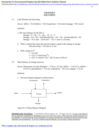
PROPRIETARY MATERIAL. © The McGraw-Hill Companies, Inc. All rights reserved. No part of this Manual
may be displayed, reproduced or distributed in any form or by any means, without the prior written permission of
the publisher, or used beyond the limited distribution to teachers and educators permitted by McGraw-Hill for their
individual course preparation. If you are a student using this Manual, you are using it without permission.
3-1
CHAPTER 3
SOLUTIONS
3-1 Lake Pleasant elevation drop
Given: Inflow = 0.0; Outflow = 0.0; Evaporation = 6.8 mm/d; Seepage = 0.01 mm/d
Solution:
a. The mass balance for the lake is
Storage = P + Qin + Iin – Qout – R – E – T
Storage = 0.0 + 0.0 – (0.01mm/d)(31d) – 0.0 – 0.0 – (6.8mm/d)(31d) – 0.0
Storage = -0.31 mm – 210.8 mm = -211.11 mm or -210 mm
b. With a vertical lake shore the elevation drop is equal to the change in storage.
Elevation drop = 210 mm or 21 cm
c. With a slope of 5˚
r = y*cscӨ
r = (211.11 mm)*csc(5˚)
r = (211.11 mm)(11.47) = 2421.4 mm or 242 cm
3-2 Mass balance on storage reservoir
Given: Dimensions of Lake Kickapoo = 12 km x 2.5 km; Inflow = 3.26 m3
/s; outflow =
2.93 m3
/s; precipitation = 15.2 cm; evaporation = 10.2 cm; seepage = 2.5 cm
Solution:
a. The mass balance diagram is shown below.
Figure S-3-2 Mass Balance Diagram
StorageInflow Outflow
Precipitation Evaporation
Seepage
Introduction To Environmental Engineering 4th Edition Davis Solutions Manual
Full Download: http://testbankreal.com/download/introduction-to-environmental-engineering-4th-edition-davis-solutions-manual/
This is sample only, Download all chapters at: testbankreal.com

3-2
b. The mass balance equation is:
∆Storage = Precipitation + Inflow - Evapotranspiration - Outflow - Seepage
c. Convert all units to volumes
Area of Lake Kickapoo = (12 km)(2.5 km) (1 x 106
m2
/km2
) = 3.0 x 107
m2
Precip. = (15.2 cm)(3.0 x 107
m2
)(10-2
m/cm) = 4.56 x 106
m3
Inflow = (3.26 m3
/s)(86,400 s/d)(31 d/mo of MAR) = 8.73 x 106
m3
Evap. = (10.2 cm)(3.0 x 107
m2
)(10-2
m/cm) = 3.06 x 106
m3
Outflow = (2.93 m3
/s)(86,400 s/d)(31 d/mo of MAR) = 7.85 x 106
m3
Seepage = (2.5 cm)(3.0 x 107
m2
)(10-2
m/cm) = 7.5 x 105
m3
d. Compute change in storage
∆Storage = 4.56 x 106
m3
+ 8.73 x 106
m3
- 3.06 x 106
m3
- 7.85 x 106
m3
- 7.5 x 105
m3
∆Storage = 1.63 x 106
m3
3-3 Mass balance on storage reservoir and runoff coefficient
Given: watershed area = 4,000 km2
; precipitation = 102 cm/y; flow of river = 34.2 m3
/s;
infiltration = 5.5 x 10-7
cm/s; evapotranspiration = 40 cm/y
Solution:
a. The mass balance diagram is shown below.

3-3
Figure S-3-3 Mass Balance Diagram
b. The mass balance equation is:
∆Storage = Precipitation - Outflow - Evapotranspiration - Infiltration.
c. It is convenient to solve the mass balance equation in units of cm/y, so converting
flow and infiltration:
( )( )( )( )
( )( ) ycm96.26
kmm101km4000
mcm100yd365ds86400sm2.34
Flow 2262
3
=
×
=
Infiltration = (5.5 x 10-7
cm/s)(86,400 s/d)(365 d/y) = 17.34 cm/y
d. Compute the change in storage.
∆Storage = 102 cm/y - 26.96 cm/y - 40 cm/y - 17.34 cm/y = 17.70 cm/y
The volume for the 4,000 km2
area,
Volume = (17.70 cm/y)(10-2
m/cm)(4,000 km2
)(1 x 106
m2
/km2
)
Volume = 7.08 x 108
m3
or 7 x 108
m3
e. The runoff coefficient is
26.0
cm102
cm96.26
ionprecipitat
runoff
C ===
Storage
Outflow
Precipitation Evapotranspiration
Infiltration

3-4
3-4 Infiltration rates and total volume
Given: Values for Horton constants for Fuquay pebbly lam sand
Solution:
a. For 12 minutes (.020 h)
f = 61 + (159 – 61) exp[(-4.7)(0.20 h)] = 99.28 or 99 mm/h
b. For 30 minutes (0.50 h)
f = 61 + (159 – 61) exp[(-4.7)(0.50 h )] = 70.35 or 70 mm/h
c. For 60 minutes (1.0 h)
f = 61 + (159 – 61) exp[(-4.7)(1.0 h)] = 61.89 or 62 mm/h
d. For 120 minutes (2.0 h)
f = 61 + (159 – 61) exp[(-4.7)(2.0 h)] = 61.00 or 61 mm/h
e. Volume over 120 minutes (2.0 h)
( )( ) ( )( )[ ]{ } mm85.14285.201220.27.4exp1
7.4
61159
261V =+=−
−
+=
3-5 Total volume of infiltration
Given: Values for Horton constants: fo = 4.70 cm/h or 47.0 mm/h; fc = 0.70 cm/h or 7.0
mm/h; k = 0.1085 h-1
and three sequential storms of 30 minute duration with
precipitation rates of 30 mm/h, 53 mm/h, and 23 mm/h.
Solution:
a. First 30 minutes
Vstorm = (30 mm/h)(0.5 h) = 15 mm
( )( ) ( )( )[ ]{ } mm97.225.01085.0exp1
1085.0
0.70.47
5.00.7Vhorton =−−
−
+=
Since the volume of precipitation is less than the infiltration, the volume of
infiltration is 15 mm
b. Second 30 minutes
Vstorm = (53 mm/h)(0.5 h) = 26.5 mm

3-5
( )( ) ( )( )[ ]{ } mm4.410.11085.0exp1
1085.0
0.70.47
−
+=
Since the volume of precipitation is 15 + 26.5 = 41.5 mm, the volume of infiltration is
41.5 mm
c. Third 30 minutes
Vstorm = (23 mm/h)(0.5 h) = 11.5 mm
( )( ) ( )( )[ ]{ } mm87.585.11085.0exp1
1085.0
0.70.47
−
+=
Since the volume of precipitation is 15 + 26.5 + 11.5 = 53.0 mm, the volume of
infiltration is 53 mm
3-6 Estimated evaporation
Given: Lake Hefner equations; air temperature= 30 °C; water temperature = 15 °C; wind
speed 9 m/s; and RH = 30 %.
Solution:
a. From Table 3-1, at 15 °C the saturation vapor pressure is estimated to be 1.704 kPa
b. Using a vapor pressure of 4.243 at 30 °C and 30 % RH, the vapor pressure in the
overlying air is estimated to be:
ea = (4.243 kPa)(0.30) = 1.2729 kPa
c. Estimated evaporation
E = 1.22(1.704 - 1.2729)(9) = 4.73 or 4.7 mm
3-7 Estimated evaporation – hot and dry
Given: Lake Hefner equations; air temperature = 40˚C; water temperature = 25˚C; wind
speed is 2.0 m/s; and relative humidity is 5 %
Solution:
a. From Table 3-1 with a water temperature of 25˚C, the saturation vapor pressure is

3-6
estimated to be 3.167 kPa
b. Using a vapor pressure of 7.378 at 40˚C and 5% RH, the vapor pressure of the
overlying air is estimated to be
ea = (7.378)(0.05) = 0.3689 kPa
c. Estimated evaporation
E = 1.22(3.167 – 0.3689)(2.0) = 6.83 or 6.8 mm/d
3-8 Estimated humidity to reduce evaporation to nil
Given: Water temperature = 10 °C; air temperature = 25 °C
Solution:
a. From Table 3-1, at 10 °C the saturation vapor pressure is 1.227 kPa
b. For E to = 0 regardless of wind speed, the values of ea and es must be equal. At 25 °C
the value of ea must be 1.227, so
ea = 1.227 = (3.167)(RH)
Solving for RH
387.0
167.3
227.1
RH == or 39 %
3-9 IDF curve for 2 y storm
Given: T = 2 y; n = 45 y; Table 3-1
Solution:
23
2
46
T
1n
m ==
+
=
Starting with the 5-minute duration, note that the 23rd ranked storm lies between the 49th
and 16th ranked storms, that is:

3-7
Intensity, mm/h
120 140
Rank 49 16
< 23 >
By interpolating find the intensity is 135.8 mm/h. Using m = 23 interpolate to find
intensities for selected durations.
Duration (min) Intensity (mm/h)
5 135.8
10 116.7
15 98.7
20 70.0
30 37.8
40 33.5
50 23.9
60 --
Given: T = 2 y ; n = 45; Table 3-1
Solution:
60.4
10
46
m ==
By interpolation find intensities for selected durations:
5 172.0
10 156.0
15 129.3
20 98.0
30 72.6
40 49.7
50 38.2
60 26.3

3-8
Given: T = 5 y; n = 10; Annual max data
Solution:
20.2
5
11
m ==
Under each duration find intensity of 2.20 ranked storm by interpolation:
Given: T = 2 y; n = 10; Annual max. data from 2-3
Solution:
50.5
2
11
==m
Under each duration find intensity of 5.50 ranked storm by interpolation:
30 82.0
60 61.2
90 41.1
120 16.2
3-13 Parking lot configuration
Given: Vertical and horizontal configurations
For “a” D = 830 m, S = 6.00 %
For “b” D = 600 m, S = 6.00 %
Solution:
a. From Table 3-3 under pavement select C = 0.95 for “asphaltic”
30 118.8
60 96.8
90 77.8
120 52.2

3-9
b. For configuration “a”
( )( )( )[ ] min75.7
817.1
08.14
00.6
83028.395.01.18.1
t
3
1
2
1
c ==
−
= or 7.8 min
c. For configuration “b”
( )( )( )[ ] min59.6
817.1
977.11
00.6
00.60028.395.01.18.1
t
3
1
2
1
c ==
−
= or 6.6 min
3-14 Mechanicsville runoff by rational method
Given: Figure P-3-14, 2 y storm and building types with areas shown in table below.
Solution:
Area Type Area (m2
) % of Total C*
Slate roofs 15831 21.39 0.95
Asphalt streets 18886 25.52 0.95
Flat (2%) sandy soil 39293 53.09 0.10
SUM 74010 100.00
*
From Table 3-3. The most conservative estimates of C are those that yield the
greatest runoff and, hence, result in the largest (most conservative) storm sewer.
Composite value for C
C = .2139(.95) + .2552(.95) + .5309(.10)
C = 0.2032 + 0.2424 + 0.0531
C = 0.4987
Calculate tc using "flat" slope of 2.0% from Eqn. 3-16
( )( )( )[ ] min65.25
2599.1
3266.32
0.2
27228.34987.01.18.1
t
3
1
2
1
c ==
−
=
From IDF Curve (Figure P-3-14) find i at Duration = 25.65 min
i = 59 mm/h
Compute peak discharge from Eqn. 3-15
Q = 0.0028(0.4987)(59)(74,010)(1 x 104 m2
/ha)
Q = 0.6097 m3
/s or 0.61 m3
/s

3-10
3-15 Mechanicsville runoff in Miami, FL
Given: Same as 3.14
Solution:
a. Calculate composite C and tc as in Problem 3.14
b. From IDF curve for Miami, FL find C at Duration = 25.65 min (0.42 h)
From Figure 3-10c read i ≅ 110 mm/h
c. Peak discharge
Q = 0.0028(0.4987)(110)(74010)(1 x 10-4
)
Q = 1.136 or 1.14 m3
/s
3-16 Little League/pasture runoff by rational method
Given:
A = 9.94 ha
D = 450 m
S = 2.00 %
C = 0.20
IDF curves from Boston, MA (Figure 3-10a)
5 year return period
Solution:
a. Compute tc
( )( )( )[ ] min398.49
2599.1
24.62
00.2
0.45028.320.01.18.1
t
3
1
2
1
c ==
−
=
b. For 5 y storm in Boston
h
h
82.0
min60
min398.49
=
From Figure 3-10a read i = 38 mm/h
c. Peak discharge
Q = 0.0028(0.20)(38)(9.94)
Q = 0.21 m3
/s

3-11
3-17 Little League/parking lot runoff
Given:
A = 2.64 ha
D = 200.0 m
S = 1.80 %
C = 0.70
IDF curves for Boston, MA (Figure 3-10a)
5 y return period
Solution:
a. Compute tc
( )( )( )[ ] min15.15
216.1
44.18
80.1
20028.370.01.18.1
t
3
1
2
1
c ==
−
=
b. From IDF curve for Boston
h
h
25.0
min60
min15.15
=
From Figure 3-10a read i = 76 mm/h
c. Peak discharge
Q = 0.0028(0.70)(76)(2.64)
Q = 0.39 m3
/s
d. Culvert does NOT have enough capacity
0.39 m3
/s > 0.21 m3
/s
3-18 Peak discharge at Holland, MI
Given:
A = 4.8 ha
D = 219.0 m
C = 0.85
S = 1.00 %
IDF curve equation for Holland, MI
Solution:
a. Calculate tc
( )( )( )[ ] min06.12
0.1
06.12
00.1
0.21928.385.01.18.1
t
3
1
2
1
c ==
−
=

3-12
b. Calculate i
hmm3.83
733.7
80.1193
706.12
80.1193
i 8.0
=
+
=
+
=
c. Peak discharge
Q = 0.0028(0.85)(83.31)(4.8)
Q = 0.95 m3
/s
3-19 Shopping mall runoff by rational method
Given: Sketch shown in Figure P-3-19 and IDF curve from Figure P-3-14
Solution:
PART I: Frequency of flooding with existing culvert
a. First calculate tc for pasture alone (Eqn. 3-16)
( )( )( )[ ] min74
0.2
100028.320.01.18.1
t
3
1
2
1
c =
−
=
b. From Fig. P-3-14 at duration = 74 min. find
i = 33 mm/h
c. Now determine design flow (maximum Q) for existing culvert from Eqn. 3-15
Q = 0.0028(0.20)(33)(40.0)
Q = 0.7392 or 0.74 m3
/s
d. Calculate tc for parking lot alone
( )( )( )[ ] min22
0.2
21.44728.370.01.18.1
t
3
1
2
1
c =
−
=
e. The intensity of rainfall that will cause flooding.
Since the tc from the parking lot is substantially less than that for the pasture, the peak
flows will not coincide and the controlling discharge will be for the shorter duration from
the parking lot. Thus, ignoring the pasture, the intensity on the parking lot that will yield
the peak discharge may be found by solving Eqn 3-15 for the intensity (i):

PROPRIETARY MATERIAL. © The McGraw-Hill Companies, Inc. All rights reserved. No part of
this Manual may be displayed, reproduced or distributed in any form or by any means, without the prior
written permission of the publisher, or used beyond the limited distribution to teachers and educators
permitted by McGraw-Hill for their individual course preparation. If you are a student using this Manual,
you are using it without permission.
3-13
( )( )( )
hmm71.37
ha0.1070.00028.0
sm7392.0
i
3
==
f. Using the tc for the parking lot and the intensity calculated in "e" and plotting the
intersection of these two lines on Figure P-3-14, find, by interpolation, that the frequency
of flooding is approximately 4 times per year.
PART II
Peak discharge for 10 y storm (again ignoring pasture because tc is so much greater):
a. From P-3-14 using tc = 22 min and freq. = 10 y
i = 100 mm/h
b. Then peak discharge (and design flow) for 10 y storm is
Q = 0.0028(0.70)(100 mm/h)(10.0 ha)
Q = 1.96 or 2.0 m3
/s
3-20 Clinic runoff by rational method
Given: Sketch shown in Figure P-3-20 and IDF curve in P-3-14.
Solution:
Part I: Frequency of flooding with existing culvert
a. Calculate the time of concentration (tc) for the pasture alone using Eqn 3-16:
( )( )( )[ ] min0.35
40.4
35028.316.01.18.1
t
3
1
2
1
c =
−
=
b. From Figure P-3-14 at a duration = 35 min and a 5 y storm find
i = 63 mm/h
c. Now calculate the design flow (maximum Q) for the existing culvert using Eqn 3-15:
Q = (0.0028)(0.16)(63 mm/h)(12.65 ha) = 0.36 m3
/s
d. Now calculate tc for the parking lot alone:

3-14
( )( )( )[ ] min6.14
70.1
83.11728.370.01.18.1
t
3
1
2
1
c =
−
=
e. The intensity of rainfall that will cause flooding.
Since the tc from the parking lot is substantially less than that for the pasture, the peak
flows will not coincide and the controlling discharge will be for the shorter duration from
the parking lot. Thus, ignoring the pasture, the intensity on the parking lot that will yield
the peak discharge may be found by solving Eqn 3-15 for the intensity (i):
( )( )( )
hmm
ha
sm
i 1.58
16.370.00028.0
36.0 3
==
f. Using the tc for the parking lot and the intensity calculated in "e" and plotting the
intersection of these two lines on Figure P-3-14, find, by interpolation, that the frequency
of flooding is approximately once every 3/4 year.
Part II
The design flow for a culvert that can handle a 10 year storm runoff from the parking lot
(again ignoring the pasture because the tc for the parking lot is so much smaller than that
for the pasture) may be found as follows:
a. From Figure P-3-14 with a tc = 14.6 min and a 10 year recurrence interval, the intensity
is found to be 127 mm/h.
b. The peak flow and, hence, the design flow is
Q = (0.0028)(0.70)(127 mm/h)(3.16 ha) = 0.79 m3
/s
3-21 Peak discharge from two adjacent parcels
Given: Figure labeled with variables
Upstream Parcel Downstream Parcel
A 3.0 ha 4.0 ha
C 0.35 0.30
D 193.5 m 100.0 m
S 1.50 % 4.40 %
Drainage ditch flows at 0.60 m/s
Drainage ditch is 200.0 m long
Seattle, WA IDF curves in Figure 3-10d

3-15
Solution:
a. Calculate runoff tc for the west parcel
( )( )( )[ ] min71.29
50.1
5.19328.335.01.18.1
t
3
1
2
1
c =
−
=
b. Calculate runoff tc for the east parcel
( )( )( )[ ] min92.15
40.4
0.10028.330.01.18.1
t
3
1
2
1
c =
−
=
c. Total tc for each parcel
( ) min26.35min55.5min71.29
mins60
1
sm60.0
m0.200
71.29traveltimett cwestc =+=











+=+=
tc(east) = 15.92 min
d. Therefore use 29.71 min as the maximum time of concentration and, hence, the
duration of the rainfall. From the Seattle, WA IDF curve at 29.71 min (0.5 h) find i =
17.5 mm/h
e. Sum the CA values
( )( ) ( )( ) 25.20.430.00.335.0CA =+=∑
f. Calculate peak discharge
Q = 0.0028(17.5)(2.25)
Q = 0.11 m3
/s
3-22 Peak discharge from three adjacent parking lots
Given: Figure labeled with variables
Storm sewer flows at 0.90 m/s. The sewer lengths are 250.0 m and 400.0 m. The 5 year
storm at Miami, FL (Figure 3-10c) is to be used.
Solution:
West Center East
A 8.0 ha 12.0 ha 6.0 ha
C 0.90 0.90 0.90
D 282.8 m 244.9 m 273.8 m
S 0.90 % 1.20 % 1.80 %

3-16
a. Calculate the runoff tc for the west lot
( )( )( )[ ] min36.11
965.0
96.10
90.0
8.28228.390.01.18.1
t
3
1
2
1
c ==
−
=
b. Calculate the total tc for the west lot
( ) min36.11min0.0min36.11traveltimett cwestc =+=+=
c. Calculate the runoff tc for the center lot
( )( )( )[ ] min60.9
063.1
203.10
20.1
9.24428.390.01.18.1
t
3
1
2
1
c ==
−
=
d. Calculate the total tc for the center lot
( ) min9.17
mins60
1
sm90.0
m400
min60.9traveltimett ccenterc =











+=+=
e. Calculate the runoff tc for the east lot
( )( )( )[ ] min87.8
216.1
788.10
80.1
8.27328.390.01.18.1
t
3
1
2
1
c ==
−
=
f. Calculate the total tc for the east lot
( ) min91.20min41.7
mins60
1
sm90.0
m0.250
min87.8traveltimett ceastc =+











+=+=
Note that the 7.41 min is the travel time calculated in “d” above for the 400.0 m from
M.H. in the center lot to the last M.H.
g. The largest total tc is 20.91 min. This is the maximum time of concentration and, thus,
is the duration of the rainfall. From the Miami, FL IDF curve find i = 120 mm/h for
the five year storm at 20.91 min (0.35 h).
h. Sum the CA values
( )( ) ( )( ) ( )( ) 40.230.690.00.1290.00.890.0CA =++=∑
i. Calculate peak discharge
Q = 0.0028(23.40)(120)
Q = 7.9 m3
/s

3-17
3-23 Unit hydrograph for Isoceles River
Given: Basin area = 14.40 km2
; stream discharge graph
Solution:
The direct runoff ordinates at 1500, 1600 and 1700 hours are shown in Figure S-3-23.
The volume may be computed by the method shown in the book or from the observation
that the area under the curve is equal to the volume and, hence, is equal to 1/2
(base)(height) of the triangle.
0
0.5
1
1.5
2
2.5
3
3.5
1300 1400 1500 1600 1700 1800 1900
Time (hr)
Flow(m3/s)
Figure S-3-23
Using the book method:
Time
Interval (h)
Total
Ord.
Base
Ord.
DRH Ord. Volume
Increment (m3
)
1430 – 1530 2.0 1.0 1.0 3600
1530 – 1630 3.0 1.0 2.0 7200
1630 – 1730 2.0 1.0 1.0 3600
SUM = 14400
Volumes were computed as in 3-25.
The unit depth as in 3-25 is
( )( )
cm10.0mcm100
kmm101km40.14
m14400
2262
3
=×
×

3-18
Compute U.H. Ord. as in 3-25
Plotting Time (h) U.H. Ord. (m3
/s-cm)
1.0 10.0
2.0 20.0
3.0 10.0
3-24 Unit hydrograph for Convex River
Given: Area of watershed = 100.0 ha; Total stream flow ordinates
Solution:
a. The volume may be computed by the method shown in the book or from the
observation that the area under the curve is equal to the volume and, hence, is equal to
(1/2)(π)(D2
/4) of the circle.
b. Using the book method
Time
Interval (h)
Total Ord.
(m3
/s)
Base Ord.
(m3
/s)
DRH Ord.
(m3
/s)
Volume
Increment (m3
)
2030 – 2130 3.0 1.5 1.5 5400
2130 – 2230 3.8 1.5 2.3 8280
2230 – 2330 4.0 1.5 2.5 9000
2330 – 0030 3.8 1.5 2.3 8280
0030 – 0130 3.0 1.5 1.5 5400
SUM = 36360
Total ordinates were provided in the problem statement. Baseline ordinates are read from
the extrapolated baseline (a horizontal line).
The volume increment is calculated as:
V = (DRH)(time interval)(3600 s/h)
For example:
V = (1.50 m3
/s)(1h)(3600 s/h) = 5400 m3
c. Determine the unit depth
( )( ) cm64.3mcm100
ham101ha100
m36360
24
3
=×
×
d. Compute the U.H. ordinates

3-19
1 h cmsm41.0
cm64.3
sm5.1 3
−=
2h cmsm63.0
cm64.3
sm3.2 3
3
−=
3h cmsm69.0
cm64.3
sm5.2 3
3
−=
4h ≡ 2h = 0.63 m3
/s-cm
5h ≡ 1h = 0.41 m3
/s-cm
3-25 Unit hydrograph for Verde River
Given: Basin area = 64.0 km2
; Stream flow data for 5 h storm
Solution: Begin by plotting stream flow data as in Figure S-3-25 on following page.
a. Plot base flow as straight line extrapolation from A to B.
b. Beginning of U.H. is at beginning of DH. Arbitrarily select time intervals as shown
and find ordinates from Figure S-3-25.
Time
Interval (h)
Total Ord.
(m
3
/s)
Base Ord.
(m
3
/s)
DRH Ord.
(m
3
/s)
Volume
Increment (m
3
)
10 to 15 1 0.4 0.6 10,800
15 to 20 3.4 0.4 3 54,000
20 to 30 6.24 0.4 5.84 210,240
30 to 40 5.77 0.4 5.37 193,320
40 to 50 4.29 0.4 3.89 140,040
50 to 60 2.72 0.38 2.34 84,240
60 to 70 1.64 0.38 1.26 45,360
70 to 80 0.79 0.3 0.49 17,640
80 to 90 0.25 0.25 0 0
Total Volume = 755,640
Total ordinate and base ordinate are read at midpoint of time interval. DRH = (Total
Ord.) - (Base Ord.). Volume increment is calculated as
For example 10-15 h
V = (0.60 m3
/s)(5 h)(3600 s/h) = 10800 m3
Determine the unit depth

3-20
( )( )
cm18.1mcm100
kmm101km64
755640
2262
=×
×
Hydrograph for Verde River
0
1
2
3
4
5
6
7
8
0 20 40 60 80 100
Time, h
Discharge,m3/s
A B
Figure S-3-25 Hydrograph for Verde River
Compute U.H. ordinates
51.0
18.1
6.0
UnitDepth
Ord.DRH
Ord.H.U ===
Time
Interval (h)
Plotting
Time (h)
U.H. Ordinate
(m
3
/s-cm)
0 to 5 2.5 0.51
5 to 10 7.5 2.54
10 to 20 15 4.95
20 to 30 25 4.55
30 to 40 35 3.29
40 to 50 45 1.98
50 to 60 55 1.07
60 to 70 65 0.42
Plotting time is time from beginning of precipitation excess. In essence
new time zero is established at point A in Figure S-3-25.

3-21
3-26 Unit hydrograph for Crimson River
Given: Basin area = 626 km2
; Stream flow data for 5 h storm
Solution: As in Problem 3-25 begin with plot. See Figure S-3-26.
Construct base flow line as in Problem 3-25. Determine direct runoff volume as in 3-25:
Total ordinate and base ordinate are read at midpoint of time interval. DRH = (Total
Ord.) - (Base Ord.). Volume increment is calculated as
For example 15-20 h
V = (2.1 m3
/s)(5 h)(3600 s/h) = 37800 m3
Determine unit depth as in 3-25
( )( )
cm40.0mcm100
kmm101km626
2486160
2262
=×
×
Time
Interval (h)
Total Ord.
(m
3
/s)
Base Ord.
(m
3
/s)
DRH Ord.
(m
3
/s)
Volume
Increment (m
3
)
15 to 20 3.5 1.4 2.1 37,800
20 to 30 15.14 1.3 13.84 498,240
30 to 40 21.55 1.2 20.35 732,600
40 to 50 15.77 1.1 14.67 528,120
50 to 60 11.03 1 10.03 361,080
60 to 70 6.88 1 5.88 211,680
70 to 80 3.46 0.9 2.56 92,160
80 to 90 1.48 0.8 0.68 24,480
90 to 100 0.77 0.77 0 0
Total Volume = 2,486,160

3-22
Hydrograph for Crimson River
0
5
10
15
20
25
0 20 40 60 80 100
Time, h
Discharge,m3/s
Figure S-3-26 Hydrograph for Crimson River
Compute U.H. Ord.
Time
Interval (h)
Plotting
Time (h)
U.H. Ordinate
(m
3
/s-cm)
0 to 5 2.5 5.29
5 to 15 10 34.85
15 to 25 20 51.24
25 to 35 30 36.94
35 to 45 40 25.25
45 to 55 50 14.81
55 to 65 60 6.45
65 to 75 70 1.71
75 to 85 80 0.00
85 to 90 90 0.00

3-23
3-27 Applying U.H. Ordinates to a storm sequence
Given: U.H. Ordinates and storm sequence
Solution:
Day Rainfall
Excess (cm)
DRH Ord. (m3
/s) Compound
Runoff (m3
/s)
1 2 3 4
1 0.30 0.04 N/A-1 N/A-2 N/A-2 0.04
2 0.20 0.23 0.02 N/A-2 N/A-2 0.25
3 0.0 0.04 0.15 N/A-2 N/A-2 0.19
4 0.0 0.0 0.03 N/A-2 N/A-2 0.03
Rainfall Excess = Precipitation - Abstractions
For day 1, R.E. = 0.50 – 0.20 = 0.30
N/A-1: Rain that falls in day 2 cannot appear in the stream the day before it rains.
N/A-2: No rain falls in days 3 and 4 so there cannot be any runoff.
3-28 Compound runoff hydrograph for Isoceles River
Given: Rainfall excess for 1st hour = 0.1 cm; for 2nd hour R.E. = 0.20 cm; for 3rd hour
R.E. = 0.05 cm; U.H. ordinates from Prob. 3-23.
Solution:
DRH OrdinatesTime R.E. (cm)
1 2 3
Compound
Runoff (m3
/s)
1 0.10 1.0 N/A N/A 1.0
2 0.20 2.0 2.0 N/A 4.0
3 0.05 1.0 4.0 0.5 5.5
4 0.0 0.0 2.0 1.0 3.0
5 0.0 0.0 0.0 0.5 0.5
3-29 Compound runoff hydrograph for Verde River (Problem 3-25)
Given: Rainfall excess of 15 mm/h for 5 h from 1500 to 2000 and 10 mm/h for 5 h from
0500 to 1000 and unit hydrograph ordinates from problem 3-25
Solution: R.E. = (15 mm/h)(5 h)/(10 mm/cm) = 7.50 cm.
Note: 1500 h = 0 h for computations.

3-24
DRH OrdinatesTime
Interval
(h)
Plotting
Time
(h)
UH Ord.
(m
3
/s-cm)
Rainfall
Excess
(cm) 1 2
Compound
Runoff (m
3
/s)
0 to 5 2.5 0.51 7.5 3.825 n/a 3.825
5 to 10 7.5 2.54 19.05 n/a 19.05
10 to 20 15 4.95 37.125 n/a 37.125
20 to 30 25 4.55 5 34.125 2.55 36.675 See Note
30 to 40 35 3.29 24.675 12.7 37.375 See Note
40 to 50 45 1.98 14.85 24.75 39.6
50 to 60 55 1.07 8.025 22.75 30.775
60 to 70 65 0.42 3.15 16.45 19.6
70 to 80 75 9.9 9.9
80 to 90 85 5.35 5.35
90 to
100 95 2.1 2.1
NOTE: The plotting time for these two points must be the same time after the start of precipitation
excess as the U.H. times, I.e. 2.5 and 7.5 h. Hence, the compound runoff will not be the sum as shown.
3-30 Compound runoff hydrograph for Crimson River
Given: Rainfall excess = 25 mm/h for 5 h and 15 mm/h for 5 h
Solution:
R.E. = (25 mm/h)(5 h)/(10 mm/cm) = 12.50 cm
R.E. = (15 mm/h)(5 h)/(10 mm/cm) = 7.50 cm
Note: 1200 h = 0 h for computations and plot

3-25
DRH Ordinates Interpolation*
Time
Interval
(h)
Plotting
Time
(h)
UH
Ord.
(m
3
/s-
cm)
Rainfall
Excess
(cm) 1 2
Compound
Runoff
(m
3
/s)
0 to 5 2.5 5.29 12.5 66.13 n/a 66.13
7.5 5.29 7.5 39.68
5 to 15 10 34.85 435.63 150.53 586.15
15 34.85 261.38
15 to 25 20 51.24 640.50 322.84 963.34
25 51.24 384.30
25 to 35 30 36.94 461.75 330.68 792.43
35 36.94 277.05
35 to 45 40 25.25 315.63 233.21 548.84
45 25.25 189.38
45 to 55 50 14.81 185.13 150.23 335.35
55 14.81 111.08
55 to 65 60 6.45 80.63 79.73 160.35
65 6.45 48.38
65 to 75 70 1.71 21.38 30.60 51.98
75 1.71 12.83
75 to 85 80 6.41 6.41
*Because of the odd offset (2.5 h) the DRH ordinates for the first and second storms do not plot at the
same time. I have linearly interpolated values from the second strom to determine runoff at the same
plotting time as the first storm. The value is used to compute compound runoff.
3-31 Reservoir volume for droughts
Given: Design volume = 7.00x106
Inflow = 3.2 m3
/s
Outflow = 2.0 m3
/s
Solution:
a. Write the mass balance equation in terms of volumes
V = (Qin)(t) – (Qout)(t)
b. Solve for t
d5.67
ds86400
1
sm0.2sm2.3
1000.7
QQ
V
t 33
6
outin
=











−
×
=
−
=

3-26
3-32 Woebegone water tower
Given: Estimeated demand cylce
Pump capacity = 36 L/s
Solution:
a.This is a mass balance problem. Set up tabular form as shown below.
Time Qin (L/s) Vin (L) Qout (L/s) Vout (L) ∆S Σ∆s
12am – 6am 36 777600* 0.0 0.0 777600 777600
6am – 12noon 36 777600 54.0** 1166400 -388800 388800
12noon – 6pm 36 777600 54.0 1166400 -388800 0.0
6pm – 12midnight 36 777600 36.0 777600 0.0 0.0
*(36 L/s)(6 h)(3600 s/h) = 777600
**(54 L/s)(6 h)(3600 s/h) = 1166400
b. Volume of water tower required is 777600 L
3-33 Water supply from Clear Fork Trinity River
Given: Table of mean monthly discharge; Demand = 0.35 m3
/s
Solution:
a. Mass balance by spreadsheet
Year Month
Qin
(m
3
/s) Qin*∆t (m
3
)
Qout
(m
3
/s)
Qout*∆t
(m
3
) ∆S (m
3
) Σ∆S (m
3
)
1951 Jul 0.98 2,624,832 0.35 937,440 1,687,392 0
Aug 0 0 0.35 937,440 -937,440 -937,440
Sep 0 0 0.35 907,200 -907,200 -1,844,640
Oct 0 0 0.35 937,440 -937,440 -2,782,080
Nov 0.006 15,552 0.35 907,200 -891,648 -3,673,728
Dec 0.09 241,056 0.35 937,440 -696,384 -4,370,112
1952 Jan 0.175 468,720 0.35 937,440 -468,720 -4,838,832 <=
Feb 0.413 999,130 0.35 846,720 152,410 -4,686,422
Mar 0.297 795,485 0.35 937,440 -141,955 -4,828,378
Apr 1.93 5,002,560 0.35 907,200 4,095,360 -733,018
May 3.65 9,776,160 0.35 937,440 8,838,720 8,105,702 <= Reservoir is full
and overflows excess
b. Volume required is 4838832 m3
c. Reservoir is full and overflows excess at end of May.

3-27
3-34 Water supply for Squannacook River
/s
Solution:
Year Month
Qin
(m
3
/s) Qin*∆t (m
3
)
Qout
(m
3
/s) Qout*∆t (m
3
) ∆S (m
3
) Σ∆S (m
3
)
1964 Jan 3.77 10,097,568 1.76 4,713,984 5,383,584 0
Feb 2.57 6,217,344 1.76 4,257,792 1,959,552 0
Mar 7.33 19,632,672 1.76 4,713,984 14,918,688 0
Apr 6.57 17,029,440 1.76 4,561,920 12,467,520 0
May 1.85 4,955,040 1.76 4,713,984 241,056 0
Jun 0.59 1,529,280 1.76 4,713,984 -3,184,704 -3,184,704
Jul 0.38 1,017,792 1.76 4,713,984 -3,696,192 -6,880,896
Aug 0.25 669,600 1.76 4,713,984 -4,044,384 -10,925,280
Sep 0.21 544,320 1.76 4,561,920 -4,017,600 -14,942,880
Oct 0.27 723,168 1.76 4,713,984 -3,990,816 -18,933,696
Nov 0.36 933,120 1.76 4,561,920 -3,628,800 -22,562,496
Dec 0.79 2,115,936 1.76 4,713,984 -2,598,048 -25,160,544
1965 Jan 0.65 1,740,960 1.76 4,713,984 -2,973,024 -28,133,568
Feb 1.33 3,217,536 1.76 4,257,792 -1,040,256 -29,173,824
Mar 2.38 6,374,592 1.76 4,713,984 1,660,608 -27,513,216
Apr 3.79 9,823,680 1.76 4,561,920 5,261,760 -22,251,456
May 1.47 3,937,248 1.76 4,713,984 -776,736 -23,028,192
Jun 0.59 1,529,280 1.76 4,713,984 -3,184,704 -26,212,896
Jul 0.23 616,032 1.76 4,713,984 -4,097,952 -30,310,848
Aug 0.2 535,680 1.76 4,713,984 -4,178,304 -34,489,152
Sep 0.19 492,480 1.76 4,561,920 -4,069,440 -38,558,592
Oct 0.27 723,168 1.76 4,713,984 -3,990,816 -42,549,408
Nov 0.45 1,166,400 1.76 4,561,920 -3,395,520 -45,944,928
Dec 0.64 1,714,176 1.76 4,713,984 -2,999,808 -48,944,736
1966 Jan 0.61 1,633,824 1.76 4,713,984 -3,080,160 -52,024,896
Feb 1.96 4,741,632 1.76 4,257,792 483,840 -51,541,056
Mar 5.55 14,865,120 1.76 4,713,984 10,151,136 -41,389,920
Apr 2.92 7,568,640 1.76 4,561,920 3,006,720 -38,383,200
May 2.46 6,588,864 1.76 4,713,984 1,874,880 -36,508,320
Jun 0.8 2,073,600 1.76 4,713,984 -2,640,384 -39,148,704
Jul 0.26 696,384 1.76 4,713,984 -4,017,600 -43,166,304
Aug 0.18 482,112 1.76 4,713,984 -4,231,872 -47,398,176
Sep 0.27 699,840 1.76 4,561,920 -3,862,080 -51,260,256
Oct 0.52 1,392,768 1.76 4,713,984 -3,321,216 -54,581,472
Nov 1.75 4,536,000 1.76 4,561,920 -25,920 -54,607,392
Dec 1.35 3,615,840 1.76 4,713,984 -1,098,144 -55,705,536

3-28
b. Volume required is 56476224 m3
c. The reservoir is not full at the end of December 1967.
3-35 Water supply from the Hoko River
/s
Solution:
Note: Flow restriction implies
10.0
Q
sm325.0
in
3
=
sm25.3
10.0
sm325.0
Q 3
3
in ==
Year Month
Qin
(m
3
/s) Qin*∆t (m
3
)
Qout
(m
3
/s) Qout*∆t (m
3
) ∆S (m
3
) Σ∆S (m
3
)
1972 May 3 8,035,200 3.25 8,704,800 -669,600 -669,600
Jun 1 2,592,000 3.25 8,704,800 -6,112,800 -6,782,400
Jul 5.32 14,249,088 3.25 8,704,800 5,544,288 -1,238,112
Aug 0.841 2,252,534 3.25 8,704,800 -6,452,266 -7,690,378
Sep 2 5,184,000 3.25 8,424,000 -3,240,000 -10,930,378
Oct 1.14 3,053,376 3.25 8,704,800 -5,651,424 -16,581,802 <=
Nov 11.8 30,585,600 3.25 8,424,000 22,161,600 5,579,798 <= reservoir is full
b. Volume or reservoir is 16,581,802 m3
1967 Jan 1.68 4,499,712 1.76 4,713,984 -214,272 -55,919,808
Feb 1.53 3,701,376 1.76 4,257,792 -556,416 -56,476,224 <=
Mar 2.64 7,070,976 1.76 4,713,984 2,356,992 -54,119,232
Apr 10.62 27,527,040 1.76 4,561,920 22,965,120 -31,154,112
May 6.29 16,847,136 1.76 4,713,984 12,133,152 -19,020,960
Jun 3.17 8,216,640 1.76 4,713,984 3,502,656 -15,518,304
Jul 2.22 5,946,048 1.76 4,713,984 1,232,064 -14,286,240
Aug 0.72 1,928,448 1.76 4,713,984 -2,785,536 -17,071,776
Sep 0.47 1,218,240 1.76 4,561,920 -3,343,680 -20,415,456
Oct 0.6 1,607,040 1.76 4,713,984 -3,106,944 -23,522,400
Nov 1.07 2,773,440 1.76 4,561,920 -1,788,480 -25,310,880
Dec 3.03 8,115,552 1.76 4,713,984 3,401,568 -21,909,312 <= Reservoir is not full yet

3-29
3-36 Bar Nunn retention pond
Given: Tabulation of inflow and outflow; Each interval is 1 h
Solution:
a. Using mass balance technique complete the table.
Interval Qin (L/s) Vin (m3
) Qout (L/s) Vout (m3
) ∆V (m3
) Σ∆V (m3)
1 10.0 36.0* 10.0 36.0 0 0
2 20.0 72.0 10.0 36.0 36.0 36.0
3 30.0 108.0 10.0 36.0 72.0 108.0
4 20.0 72.0 10.0 36.0 36.0 144.0
5 15.0 54.0 10.0 36.0 18.0 162.0
6 5.0 18.0 10.0 36.0 Outflow exceeds inflow
*Example calculation
(10.0 L/s)(1 h)(3600 s/h)(1x10-3
m3
/L) = 36.0 m3
b. The maximum V is 162.0 m3
. Therefore, the volume of the retention basin should be
162.0 m3
.
3-37 Menominee River flood storage
Given: Table of mean monthly discharges January 1, 1959 – December 31, 1960.
Flood stage is at 100 m3
/s
Downstream discharge is 100 m3
/s
Solution:
a. Mass balance by spreadsheet (following page)

3-30
Year Month
Qin
(m
3
/s) Qin*∆t (m
3
)
Qout
(m
3
/s) Qout*∆t (m
3
) ∆S (m
3
) Σ∆S (m
3
)
1959 Jan 46.7 125,081,280 100 267,840,000 -142,758,720 0
Feb 43.1 104,267,520 100 241,920,000 -137,652,480 0
Mar 55 147,312,000 100 267,840,000 -120,528,000 0
Apr 110 285,120,000 100 259,200,000 25,920,000 25,920,000
May 105 281,232,000 100 267,840,000 13,392,000 39,312,000
Jun 56.7 146,966,400 100 259,200,000 -112,233,600 0
<= Reservoir
completely
empty at end
of JUN
Jul 48.3 129,366,720 100 267,840,000 -138,473,280 0
Aug 78 208,915,200 100 267,840,000 -58,924,800 0
Sep 142 368,064,000 100 259,200,000 108,864,000 108,864,000
Oct 155 415,152,000 100 267,840,000 147,312,000 256,176,000
Nov 122 316,224,000 100 259,200,000 57,024,000 313,200,000
Dec 78.2 209,450,880 100 267,840,000 -58,389,120 254,810,880 See note
1960 Jan 82.3 220,432,320 100 267,840,000 -47,407,680 207,403,200 See note
Feb 71 171,763,200 100 241,920,000 -70,156,800 137,246,400 See note
Mar 62.4 167,132,160 100 267,840,000 -100,707,840 36,538,560 See note
Apr 242 627,264,000 100 259,200,000 368,064,000 404,602,560
May 373 999,043,200 100 267,840,000 731,203,200 1,135,805,760
Jun 135 349,920,000 100 259,200,000 90,720,000 1,226,525,760 <= max. vol
Jul 83.4 223,378,560 100 267,840,000 -44,461,440 1,182,064,320
Aug 72.1 193,112,640 100 267,840,000 -74,727,360 1,107,336,960
Sep 80.8 209,433,600 100 259,200,000 -49,766,400 1,057,570,560
Oct 60.5 162,043,200 100 267,840,000 -105,796,800 951,773,760
Nov 102 264,384,000 100 259,200,000 5,184,000 956,957,760
Dec 68.2 182,666,880 100 267,840,000 -85,173,120 871,784,640
<= Reservoir not
empty at end
of DEC
NOTE: Although Qin is less than 100 m3
, the reservoir is not empty at the end of DEC (or JAN, FEB,
MAR).
b. Volume required is 1,226,525,760 m3
3-38 Spokane River flood storage
Given: Table of mean monthly discharges for March 1957 through October 1958
Flood stage is ≥ 250 m3
/s
Discharge is 250 m3
/s for each flood
Solution:

3-31
Year Month
Qin
(m
3
/s) Qin*∆t (m
3
)
Qout
(m
3
/s) Qout*∆t (m
3
) ∆S (m
3
) Σ∆S (m
3
)
1957 Jan 99 265,161,600 250 669,600,000 -404,438,400 0
Feb 61 147,571,200 250 604,800,000 -457,228,800 0
Mar 278 744,595,200 250 669,600,000 74,995,200 74,995,200
Apr 461 1,194,912,000 250 648,000,000 546,912,000 621,907,200
May 792 2,121,292,800 250 669,600,000 1,451,692,800 2,073,600,000
Jun 329 852,768,000 250 648,000,000 204,768,000 2,278,368,000 <= max. vol
Jul 33.6 89,994,240 250 669,600,000 -579,605,760 1,698,762,240
Aug 12.5 33,480,000 250 669,600,000 -636,120,000 1,062,642,240
Sep 15.7 40,694,400 250 648,000,000 -607,305,600 455,336,640
Oct 55.5 148,651,200 250 669,600,000 -520,948,800 0
<= Reservoir
completely empty
by end of OCT
Nov 66.9 173,404,800 250 648,000,000 -474,595,200 0
Dec 73 195,523,200 250 669,600,000 -474,076,800 0
1958 Jan 80 214,272,000 250 669,600,000 -455,328,000 0
Feb 245 592,704,000 250 604,800,000 -12,096,000 0
Mar 234 626,745,600 250 669,600,000 -42,854,400 0
Apr 408 1,057,536,000 250 648,000,000 409,536,000 409,536,000
May 548 1,467,763,200 250 669,600,000 798,163,200 1,207,699,200
Jun 152 393,984,000 250 648,000,000 -254,016,000 953,683,200
Jul 29.5 79,012,800 250 669,600,000 -590,587,200 363,096,000
Aug 4.5 12,052,800 250 669,600,000 -657,547,200 0
<= Reservoir not
empty at end
of AUG
Sep 24.4 63,244,800 250 648,000,000 -584,755,200 0
Oct 36.8 98,565,120 250 669,600,000 -571,034,880 0
Nov 153 396,576,000 250 648,000,000 -251,424,000 0
Dec 240 642,816,000 250 669,600,000 -26,784,000 0
b. Storage required = 2.28 x 109
m3
c. The reservoir is not empty.
3-39 Rappahannuck River flood storage
Given: Table of mean monthly discharge
Flood stage is 5.8 m3
/s
Downstream discharge is constant at average flow for the period
Solution:

3-32
Year Month
Qin
(m
3
/s) Qin*∆t (m
3
)
Qout
(m
3
/s) Qout*∆t (m
3
) ∆S (m
3
) Σ∆S (m
3
)
1960 Jan 4.11 11,008,224 5.8 15,534,720 -4,526,496 0
Feb 9.71 23,490,432 5.8 14,031,360 9,459,072 9,459,072
Mar 7.7 20,623,680 5.8 15,534,720 5,088,960 14,548,032
Apr 13.3 34,473,600 5.8 15,033,600 19,440,000 33,988,032
May 11.3 30,265,920 5.8 15,534,720 14,731,200 48,719,232
Jun 9.97 25,842,240 5.8 15,033,600 10,808,640 59,527,872
Jul 2.97 7,954,848 5.8 15,534,720 -7,579,872 51,948,000
Aug 1.85 4,955,040 5.8 15,534,720 -10,579,680 41,368,320
Sep 2.77 7,179,840 5.8 15,033,600 -7,853,760 33,514,560
Oct 1.1 2,946,240 5.8 15,534,720 -12,588,480 20,926,080
Nov 1.23 3,188,160 5.8 15,033,600 -11,845,440 9,080,640
Dec 1.31 3,508,704 5.8 15,534,720 -12,026,016 0
<= Reservoir completely
empty by end of DEC
1961 Jan 3.31 8,865,504 5.8 15,534,720 -6,669,216 0
Feb 15.4 37,255,680 5.8 14,031,360 23,224,320 23,224,320
Mar 9.85 26,382,240 5.8 15,534,720 10,847,520 34,071,840
Apr 15.5 40,176,000 5.8 15,033,600 25,142,400 59,214,240
May 11.1 29,730,240 5.8 15,534,720 14,195,520 73,409,760
Jun 6.82 17,677,440 5.8 15,033,600 2,643,840 76,053,600
Jul 3.23 8,651,232 5.8 15,534,720 -6,883,488 69,170,112 <= max. vol
Aug 2.24 5,999,616 5.8 15,534,720 -9,535,104 59,635,008
Sep 1.7 4,406,400 5.8 15,033,600 -10,627,200 49,007,808
Oct 1.16 3,106,944 5.8 15,534,720 -12,427,776 36,580,032
Nov 1.77 4,587,840 5.8 15,033,600 -10,445,760 26,134,272
Dec 4.25 11,383,200 5.8 15,534,720 -4,151,520 21,982,752
1962 Jan 5.44 14,570,496 5.8 15,534,720 -964,224 21,018,528
Feb 5.61 13,571,712 5.8 14,031,360 -459,648 20,558,880
Mar 16.8 44,997,120 5.8 15,534,720 29,462,400 50,021,280
Apr 10.7 27,734,400 5.8 15,033,600 12,700,800 62,722,080
May 5.27 14,115,168 5.8 15,534,720 -1,419,552 61,302,528
Jun 6.88 17,832,960 5.8 15,033,600 2,799,360 64,101,888
Jul 3.57 9,561,888 5.8 15,534,720 -5,972,832 58,129,056
Aug 1.51 4,044,384 5.8 15,534,720 -11,490,336 46,638,720
Sep 0.855 2,216,160 5.8 15,033,600 -12,817,440 33,821,280
Oct 0.932 2,496,269 5.8 15,534,720 -13,038,451 20,782,829
Nov 4.73 12,260,160 5.8 15,033,600 -2,773,440 18,009,389
Dec 3.6 9,642,240 5.8 15,534,720 -5,892,480 12,116,909
b. Storage required = 6.92 x 107
m3

3-33
3-40 Hydraulic gradient size and direction
Given: A 100 ha square; total piezometric head at each corner.
Solution:
a. Determine the dimensions of the square by converting to m2
and taking square root.
Area = (100 ha)(104
m2
/ha) = 1.0 x 106
m2
Distance between wells = length of side = (1.0 x 106
m2
)0.5
= 1,000 m
b. The hydraulic gradient is exactly from west to east because both western total heads
and the eastern total heads are the same. There is no need to plot the points. Either the
NE/NW line or the SE/ SW line can be used to calculate the magnitude of the
hydraulic gradient:
4
100.6
1000
306.30
radientHydraulicG −
×=
−
=
3-41 Hydraulic gradient size and direction
Given: Same wells as in Problem 3-40; water levels measured from ground surface.
Solution:
a. Distances are the same as Problem 3-40.
b. Note that water elevations are measured from the surface, so the gradient is from the
east to the west. The NW corner is 0.4 below the NE and SE corners and the SW
corner is 0.6 m below the NE and SE corners.
c. The flow pattern is a little more complex. Since the total head at the NE corner is the
same as that of the SE corner, a point midway between the two corners is assumed to
have the same total head. Begin the construction with the point midway between the
NE and SE corners and the other two corners as shown below.

3-34
Figure S-3-41
d. Graphically determine the distance from A to B to be 370 m and calculate the
hydraulic gradient as:
4
104.5
370
4.06.0
radientHydraulicG −
×=
−
=
3-42 Hydraulic gradient for modeling study
Given: Well grid; ground surface elevation; and depth to ground water table in each well.
Solution:
a. Note that water elevations are measured from the surface
b. Plot the wells and elevations as shown below
NW
-0.4
SW
-0.6
NE
0.0
SE
0.0
0.0
370

3-35
Figure S-3-42
c. Follow directions given under “Definition of Terms” in Section 3-5. The graphical
construction is shown on the next page.
The calculation of the pont on CA with head equal to B is as follows:
00066.0
500
33.0
m500
52.585.5
==
−
5.85 – 5.52 = 0.33
5.63 – 5.52 = 0.11
5.85 – 5.63 = 0.22
0.33/500 = 0.00066 m/m
0.22/0.00066 = 333.33
0.11/0.00066 = 166.67
Sum = 500
333.33 m
166.67 m
A
-5.85
B
-5.63
C
-5.52
r
α
280.0 m
Direction of flow

3-36
m67.166
00066.0
11.0
00066.0
52.563.5
==
−
Measure 166.67 m from point C to point of equal head.
500 – 166.67 = 333.33
d. Calculate the distance
( )
0.280
33.333
tan 1
=α−
α = 49.97˚
The distance is then r = 280.0*sin(α) = 280.0*sin(49.97) = 214.396 m
00103.0
396.214
63.585.5
radientHydraulicG =
−
=
3-43 Darcy velocity
Given: hydraulic conductivity = 6.9 x 10-4
m/s; hydraulic gradient = 0.00141; porosity =
0.20
Solution:
a. The Darcy velocity is given by Equation 3-21
v = (6.9 x 10-4
m/s)(0.00141) = 9.73 x 10-7
m/s
b. The average linear velocity is given by Equation 3-25
sm1086.4
20.0
sm1073.9
v 6
7
−
−
×=
×
=′
3-44 Darcy velocity for fine sand
Given: hydraulic conductivity = 3.5 x 10-5
m/s; hydraulic gradient = 0.00141; porosity =
0.45
Solution:
a. Darcy velocity is given by Equation 3-21
v = (3.5 x 10-5
m/s)(0.00141) = 4.94 x 10-8
m/s
b. Average linear velocity is given by Equation 3-25

3-37
3-45 Darcy velocity and hydraulic gradient
Given: Average linear velocity = 0.60 m/d; porosity = 0.30; hydraulic
conductivity = 4.75 x 10-4
m/s
Solution:
a. Solve Equation 3-25 for the Darcy velocity
v = (v’)(porosity)
v = (0.60 m/d)(0.30) = 0.18 m/d
In m/s
v = (0.18 m/d)/(86400 s/d) = 2.08 x 10-6
m/s
b. Solve Equation 3-21 for the hydraulic gradient
00439.0
sm1075.4
sm1008.2
k
v
dr
dh
4
6
=
×
×
== −
−
3-46 Travel time in an aquifer
Given: two piezometers 280 m apart; difference in levels = 1.4 m; hydraulic
conductivity = 50 m/d; porosity = 0.20
Solution:
a. First compute the Darcy velocity
dm25.0
m280
m4.1
dm50v =





=
b. Compute the average linear velocity as
dm25.1
20.0
dm25.0
v ==′
3-47 Steady-state drawdown for artesian aquifer
Given: Artesian aquifer 28.0 m thick; piezometric surface 94.05 m above the confining
layer; pumping rate of 0.00380 m3
/s; drawdown of 64.05 m at observation well
48.00 m away; sandstone aquifer.
Find: Drawdown at observation well 68.00 m away.
Solution:
A sketch of the problem is shown below

3-38
Figure S-3-47
a. From the aquifer material (sandstone) and Table 3-5, find that the hydraulic
conductivity (K) is 5.8 x 10-7
.
b. Calculate h1
h1 = 94.05 m - 64.05 m = 30.00 m
c. Using Eqn 3-28 and T = KD = (5.8 x 10-7
)(28.0 m) = 1.624 x 10-5
m2
/s
( )( )






−×π
=
−
00.48
00.68
ln
m00.30hsm10624.12
00380.0 2
25
d. Solve for h2
( )
( ) m97.4200.3097.1200.30
10624.12
00.48
00.68
ln00380.0
00.30
T2
r
r
ln)Q(
h 5
1
2
2 =+=+
×π












=+
×π×














= −
e. Compute the drawdown
s2 = 94.05 - 42.97 = 51.08 m

3-39
3-48 Steady-state drawdown in artesian aquifer
Given: Artesian aquifer 99.99 m thick; piezometric surface 170.89 m above bottom
confining layer; pumping rate of 0.0020 m3
/s; drawdown of 12.73 m at well
280.0 m away; sandstone aquifer.
Solution:
Sketch is similar to 3-47 with furthest well 1492.0 m away.
a. From the aquifer material (sandstone) in Table 3-5 find a hydraulic conductivity of 5.8
x 10-7
m/s
b. Calculate h1
h1 = 170.89 – 12.73 = 158.16 m
c. Using Equation 3-28
and T = KD = (5.8 x 10-7
m/s)(99.99 m) = 5.80 x 10-5
m2
/s
Solve Equation 3-28 for h2
( ) ( )
( )
m35.16716.15819.916.158
1080.52
m0.280
m0.1492
lnsm0020.0
16.158
T2
r
r
lnQ
h 5
3
1
2
2 =+=+
×π






=+
π






= −
d. The drawdown is
s2 = 170.89 – 167.35 = 3.54 m
3-49 Steady-state artesian drawdown
Given: Artesian aquifer 42.43 m thick; piezometric surface 70.89 m above bottom
confining layer; pumping rate of 0.0255 m3
/s; drawdown of 5.04 m in well 272.70
m from the pumping well; fractured rock aquifer.
Solution:
Sketch similar to that for Problem 3-47 but the unknown drawdown is between the
pumping well and the observation well given at r1 = 64.28 m
a. From the aquifer material (fractured rock), in Table 3-5 find a hydraulic conductivity
of 5.8 x 10-5
m/s

3-40
b. Calculate h2
h2 = 70.89 – 5.04 = 65.85
c. Using Equation 3-28
and T = KD = (5.8 x 10-5
m/s)(42.43 m) = 2.46 x 10-3
m2
/s
Solve Equation 3-28 for h1
( ) ( )
( ) 47.6338.285.65
1046.22
28.64
70.272
ln0255.0
85.65
T2
r
r
lnQ
hh 3
1
2
21 =−=
×π






−=
π






−= −
d. The drawdown is
s = 70.89 – 63.47 = 7.42 m
3-50 Hydraulic conductivity of a confined aquifer
Given: Confined aquifer 82.0 m thick; drawdown of 3.55 m at 41.0 m away; drawdown
of 1.35 m at 63.5 m away; pumping rate of 0.0280 m3
/s; non-pumping
piezometric surface = 109.5 m
Solution:
a. Calculate h1 and h2
h1 = 109.5 – 3.55 = 105.95 m
h2 = 109.5 – 1.35 = 108.15 m
b. Solve Equation 3-28 for T
( )
( )
( )
( )
sm1086.8
82.13
0122.0
95.10515.1082
0.41
5.63
ln280.0
hh2
r
r
lnQ
T 24
12
1
2
−
×==
−π






=
−π






=
c. Solve T = KD for K
sm1008.1
m0.82
sm1086.8
D
T
K 5
24
−
−
×=
×
==
3-51 Steady-state drawdown to aquiclude (Qmax ?)
Given: Example Prob. 3-10; drawdown at (h1) observation well 2.0 m from pumping
well is lowered to bottom of aquiclude
Solution:
A sketch of the problem is shown below

3-41
Figure S-3-51
a. From Example Problem 3-10: K = 1.5 x 10-4
m/s
b. As in example problem
h1 = 40.0 - 10.0 = 30.0 m
h2 = 40.0 - 1.0 = 39.0 m
( )( )( ) sm0184.0
61.4
1048.8
m0.2
m0.200
ln
m0.30m0.39m0.10sm105.12
Q 3
24
=
×
=






−×π
=
−−
3-52 Radius of steady-state drawdown of 2.0 m
Given: Artesian aquifer 5 m thick; aquifer material is mixture of sand and gravel;
piezometric surface 65 m above confining layer; drawdown of 7 m at observation
well 10 m from pumping well; pumping rate is 0.020 m3
/s
Solution:
A sketch of the problem is shown below.
R1 = 2.0 m
10.0 m
40.0 m
S2 = 1.0 m
K
Pumping well
R 2 = 200.00 m

3-42
Figure S-3-52
a. From Table 3-5 with "sand and gravel” aquifer material find: K = 6.1 x 10-4
m/s
b. The transmissibility is:
T = KD = (6.1 x 10-4
m/s)(5 m) = 0.00305 m2
/s
c. Calculate heights above confining layer
h1 = 65.0 - 2.0 = 63.0 m
h2 = 65.0 - 7.0 = 58.0 m
d. Setup Eqn. 3-29
( )( )






−×π
=
−
0.10
r
ln
m0.58m0.63sm1005.32
sm020.0
2
23
3
e. Solve for r2
( )( )
sm020.0
m0.58m0.63sm1005.32
0.10
r
ln 3
25
2 −×π
=





−
Taking exponential of both sides of eqn.
( )( ) ( ) 41.12079.4exp
sm020.0
m0.58m0.63sm1005.32
exp
0.10
r
3
23
2
==





 −×π
=





−
r2 = (10.0)(120.41) = 1204.1 or 1200 m
S1 = 7.0 m
R 2 = ?
R1 = 10.0 m
5.0 m
65.0 m
K
Pumping well
S2 = 2.0 m

3-43
3-53 Steady-state unconfined aquifer hydraulic conductivity
Given: Depth of well = 18.3 m; static water level = 4.57 m below grade; test well
pumped at rate of 0.0347 m3/s; drawdown at observation wells: 2.78 m at
distance of 20 m; 0.73 m at distance of 110.0 m
Solution:
A similar sketch of the problem can be found in Problem 3-54
a. Calculate depth of aquifer
D = 18.3 – 4.57 = 13.73 m
b. Calculate h1 and h2
h1 = 13.73 – 2.78 = 10.95 m
h2 = 13.73 – 0.73 = 13.0 m
c. Solve Equation 3-29 for K
( )
( )
( )
( ) ( )[ ] sm1084.3
1054.1
1092.5
m95.10m0.13
0.20
0.110
lnsm0347.0
hh
r
r
lnQ
K 4
2
2
22
3
2
1
2
2
1
2
−
−
×=
×
×
=
−π






=
−π






=
3-54 Steady-state drawdown to bottom of aquifer
Given: Example Prob. 3-12; s1 = 30.0 m
Solution:
Figure S-3-54

3-44
a. From the example problem: K = 6.4 x 10-3
b. Calculate heights above confining layer
h1 = 30.0 - 30.0 = 0.0 m
h2 = 30.0 - 9.90 = 20.10 m
c. Calculate the maximum pumping rate
( ) ( )( )[ ] sm36.1
9915.5
1231.8
m25.0
m0.100
ln
m0.0)m10.20sm104.6
Q 3
223
==






−×π
=
−
3-55 Contractor dewatering unconfined aquifer
Given: Q = 0.0280 m3
/s; aquifer = medium sand; dimensions shown on drawing below
Solution:
A sketch of the problem is shown below. From number of days of pumping (1066)
assume that this is steady-state.
Figure S-3-55
a. Using Table 3-5 and "medium sand" find: K = 1.5 x 10-4
m/s
b. Calculate heights above confining layer
h1 = 14.05 - 9.52 = 4.53 m (h1)2
= 20.52
S1 = 9.52 m
R1 = 10.0 m
Pumping well
S2 = 4.81 m
R 2 = ?
14.05 m

3-45
h2 = 14.05 - 4.81 = 9.24 m (h2)2
= 85.38
c. Setup Eqn. 3-30
( )( )






−×π
=
−
0.10
r
ln
52.2038.85sm105.1
sm0280.0
2
24
3
e. Solve for r2
( )( )
sm0280.0
52.2038.85sm105.1
0.10
r
ln 3
24
2 −×π
=





−
Taking exponential of both sides of eqn.
( )( ) { } 9790.20916.1exp
sm0280.0
52.2038.85sm105.1
exp
0.10
r
3
24
2
==





 −×π
=
−
( )( ) m79.299790.20.10r2 ==
3-56 Dewatering aquifer
Given: Unconfined, steady-state, lower piezometric surface 5.25 m below static at 45.45
m from well and 2.50 m at 53.56 m; aquifer material is loam.
Solution:
a. Calculate heights above confining layer
h1 = 30.0 – 5.25 = 24.75 m
h2 = 30.0 – 2.50 = 27.50 m
b. From Table 3-5 find K = 6.4 x 10-6
m/s for loam soil
c. Set up Eqn. 3-30 and solve for Q
( )( ) ( )[ ]
( )
sm0176.0
164.0
1089.2
18.1ln
1089.2
45.45
56.53
ln
75.245.27104.6
Q 3
33226
=
×
=
×
=






−×π
=
−−−

3-46
3-57 Height of piezometric surface
Given: Unconfined aquifer 20 m thick; K = 1.5 x 10-4
; pumping rate is 0.015 m3
/s;
drawdown at 0.25 m diameter well is 8.0 m.
Find: Height of piezometric surface 80.0 m away.
Solution:
Figure S-3-57
a. Calculate height above confining layer
h1 = 20.0 - 8.0 = 12.0 m (h1)2
= 144.0
b. Setup Eqn. 3-30 (Note that r1 = diameter/2)
( )( )( )






−×π
=
−
125.0
0.80
ln
0.144hsm105.1
sm0150.0
2
2
24
3
c. Solve for h2
( )
( ) 73.3490.144
1071.4
1069.9
0.144
sm105.1
125.0
0.80
lnsm0150.0
h 4
2
24
3
2
2 =+
×
×
=+
×π






= −
−
−
m70.1873.349h2 ==
S1 = 8.0 mPumping well
H2 = ?
R1 = 0.5(diameter) = 0.125 m
20.0 m
R 2 = 80.0 m

3-47
3-58 Height of piezometric surface (0.5 m diameter well)
Given: See Problem 3-57; new well diameter
Solution:
a. Sketch is same as Problem 3-57
b. Set up Eqn. 3-30 (Note that r1 = diameter/2)
( )( )[ ]






−×π
=
−
250.0
0.80
ln
0.144hsm105.1
sm0150.0
2
2
4
3
c. Solve for h2
( )
( ) 61.3270.1446.1830.144
1071.4
1065.8
0.144
105.1
250.0
0.80
ln0150.0
h 4
2
4
2
2 =+=+
×
×
=+
×π






= −
−
−
m10.1861.327h2 ==
3-59 Unsteady flow in a confined aquifer
Given: Aquifer thickness = 28.00 m; aquifer material is fractured rock; drawdown in
pumping well is 6.21 m after 48 hours of pumping; pumping rate is 0.0075 m3
/s
Solution:
a. From Table 3-5 find K = 5.8 x 10-5
m/s
b. Note from Eqn. 3-30 that T = KD and calculate transmissivity
T = KD = (5.8 x 10-5
m/s)(28.00 m) = 1.62 x 10-3
m2
/s
c. Convert 48 hour pumping time to days so units are consistent
(48 h)/(24 h/d) = 2 d
d. Solve Eqn. 3-35 for s2
( ) ( )( ) m38.721.618.31068.321.6
2
48
ln
sm1062.14
sm0075.0
s 1
23
3
2 =+×=+





×π
= −
−
Note: Well diameter is not relevant for solution.

3-48
3-60 Transmissibility from pumping data (unsteady flow)
Given: Well dia. = 0.61 m; Q = 0.0303 m /s; s = 0.98 m at 8 min; s = 3.87 m at 24 h
Solution: (following example 3-10)
( )
( ) ( )0.180ln
3168.36
sm0303.0
min8
hmin60h24
ln
m98.0m87.34
sm0303.0
T
33
=





−π
=
( ) sm1033.41929.5000834.0T 23−
×==
3-61 Transmissivity of confined aquifer
Given: Pumping rate = 0.0076 m3
/s; drawdown at 0.10 min = 3.00m and at 1.00 min =
34.0 m
Solution:
a. Use Eqn 3-36
( )
( )( ) sm1049.430.21095.1
10.0
00.1
ln
m0.3m0.344
sm0076.0
T 255
3
−−
×=×=





−π
=
Note: Diameter of well is not relevant for solution.
3-62 Storage coefficient from pumping data
Given: At 96.93 m drawdown = 1.04 m after 80 min of pumping at 0.0170 m /s; t0 = 0.6
min; T = 5.39 x 10-3
m2
/s
Solution: (following example 3-13)
( )( )( )( )
( )2
23
93.96
mins60min6.0sm1039.525.2
S
−
×
=
)!NoUnits(10647.4
10395.9
4366.0
S 5
3
−
×=
×
=
Check u assumption
( ) ( )
( )( )( )
3
2
1
3
52
102.4
10305.1
10366.4
mins60min801039.54
10647.493.96
u −
−
−
−
×=
×
×
=
×
×
=
u = 4.2 x 10-3
< 0.01 , therefore okay.

3-49
3-63 Drawdown at observation well
Given: Data in Problem 3-62; 80 days of pumping
Solution:
a. Using Equation 3-35
( )
( )






×π
=− −
min80
dmin1440d80
ln
1039.54
sm0170.0
m04.1s 3
3
2
( ) ( )( ) m87.204.127.72510.004.11440ln
0677.0
0170.0
s2 =+=+=
3-64 Drawdown at pumping well
Given: T = 2.51 x 10-3
m2
/s; S = 2.86 x 10-4
; well diameter is 0.5 m; pumping rate is
0.0194 m3
/s; two days of pumping.
Solution:
a. Calculate u (see Eqn. 3-31) using r = well diameter/2
( ) ( )
( )( )( )
8
3
5
3
42
1003.1
1073.1
1079.1
ds86400d21051.24
1086.2m25.0
u −
−
−
−
×=
×
×
=
×
×
=
b. At this point two solution techniques are possible. One is to work the problem using
the W(u) method of Eqn. 3-31. The other is to recognize that u is << 0.01 and use
Eqn. 3-34. Although not required in the problem statement, both methods are
employed here.
c. By the exact W(u) method.
Using u as calculated above and Table 3-6 find
W(u) = 17.8435
Compute drawdown using Eqn. 3-31
( )( )8435.17
sm1051.24
sm0194.0
s 23
3
−
×π
=
( )( ) m97.108435.17615.0s ==

3-50
d. By the approximation of Eqn. 3-34
( )
( )( )( )
( ) ( ) 







×
×
×π
= −
−
− 42
23
23
3
1086.225.0
ds86400d2sm1051.225.2
ln
sm1051.24
sm0194.0
s






×
×
×
= −− 5
2
2
1079.1
1076.9
ln
1015.3
0194.0
s
( ) ( ) ( )( ) m96.108.17615.01046.5ln615.0s 7
==×=
3-65 Storage coefficient from pumping test data
Given: Q = 0.0350 m3
/s; r = 300.0 m; drawdown values at three time intervals.
Solution:
Using the first and last times and following Example 3-13
a. Calculate transmissibility
( )
( )0.17ln
1858.35
0350.0
min100
min1700
ln
m10.3m90.54
sm0350.0
T
3
=





−π
=
( ) sm10818.2833.200099.0T 23−
×==
b. From plot below determine t0 = 4.4 min

3-51
Estimation of Virtual Time
-2
-1
0
1
2
3
4
5
6
7
1 10 100 1000 10000
Time, min
Drawdown,m
t(0) = 4.4 min
Figure S-3-65
c. Calculate storage coefficient
( )( )( ) )!NoUnits(109.1
100.9
674.1
300
mins60min4.410818.225.2
S 5
42
3
−
−
×=
×
=
×
=
Given: Data in Problem 3-65; observation well 100.0 m form pumping well
Solution:
a. Calculate T as in Prob. 3-65 solution.
T = 2.818 x 10-3
m2
/s.
b. Use t0 from Prob. 3-65 solution.
( )( )( ) ( ))!NoUnits1067.1
100.1
674.1
100
mins60min4.410818.225.2
S 5
42
3
−
−
×=
×
=
×
=

3-52
Given: Q = 0.0221 m3
/s; r = 100.0 m; drawdown values at three time intervals.
Solution: Using the first and last times and following Example 3-13
a. Calculate transmissibility
( )
( ) sm10766.10.144ln
2035.62
0221.0
min10
min1440
ln
m35.1m30.64
sm0221.0
T 23
3
−
×==





−π
=
b. From plot below determine t0 = 2.5 min
0
1
2
3
4
5
6
7
1 10 100 1000 10000
Time, min
Drawdown,m
t(0) = 2.5 min
Figure S-3-67
( )( )( )
( )
( )!NoUnits1096.5
101
5960.0
m100
mins60min5.2sm10766.125.2
S 5
42
23
−
−
×=
×
=
×
=

3-53
Given: Data in Problem 3-67; observation well 60.0 m form pumping well
Solution:
a. Calculate T as in Prob. 3-67 solution.
T = 1.766 x 10-3
m2
/s.
b. Use t0 from Prob. 3-67 solution.
( )( )( )
( )
( )!NoUnits10656.1
106.3
5960.0
m0.60
mins60min5.2sm10766.125.2
S 4
32
23
−
−
×=
×
=
×
=
3-69 Storage coefficient from pumping data
Given: 0.76 m diameter well pumping at 0.0035 m3
/s; drawdown at three time intervals
Solution:
a. Using the first and last time and following Example 3-14, calculate the tranmissivity
( )
( )( ) sm1063.391.31028.9
20.0
0.10
ln
m00.2m00.54
sm0035.0
T 245
3
−−
×=×=





−π
=
b. From plot of drawdown versus time below find t0 = 0.015 min

3-54
y = 0.7672Ln(x) + 3.2391
0
1
2
3
4
5
6
0.01 0.1 1 10
Time, min
Drawdown,m
t(0) = 0.015 min
Figure S-3-69
c. Calculate storage coefficient using Eqn. 3-37
Note that r = (0.76 m)/2 = 0.38 m
( )( )( )
( )
( )!NoUnits1009.5
144.0
1035.7
m38.0
mins60min015.0sm1063.325.2
S 3
4
2
24
−
−−
×=
×
=
×
=
3-70 Interference of well A on B
Given: Wells 106.68 m apart; QA = 0.0379 m3
/s; T = 4.35 x 10-3
m2
/s; S = 4.1 x 10-5
Solution:
a. Calculate u
( ) ( )
( )( )( )
7
5
1
23
52
1050.8
1049.5
1067.4
ds86400d365sm1035.44
101.4m68.106
u −
−
−
−
×=
×
×
=
×
×
=
b. From Table 3-6 find W(u) = 13.4008
c. Calculate interference
( ) m29.94008.13
sm1035.44
sm0379.0
s 23
3
AonB =×
×π
= −

3-55
3-71 Total drawdown in well B
Given: Data in Prob. 3-70
Solution:
a. Calculate u for well B (r = 0.460/2 = 0.230)
( ) ( )
( )( )( ) 5
6
3
52
1049.5
101689.2
ds86400d3651035.44
101.4230.0
u
×
×
=
×
×
=
−
−
−
u = 3.95 x 10-12
c. Calculate drawdown in well B pumping alone
( )
( ) m83.116675.25
1035.44
0252.0
s 3B =
×π
= −
d. Total drawdown in well B
sTotal in B = sB + sA on B
where sA on B was determined in Prob. 3-70
sTotal in B = 11.83 + 9.29 = 21.12 m
3-72 Interference of well 12 on 13
Given: Wells 100.0 m apart; Q12 = 0.0250 m3
/s; T = 1.766 x 10-3
m2
/s; S = 6.675 x 10-5
Solution:
a. Calculate u
( ) ( )
( )( )( ) 5
1
3
52
10709.1
10675.6
ds86400d28010766.14
10675.6100
u
×
×
=
×
×
=
−
−
−
u = 3.906 x 10-6

3-56
c. Calculate interference
( )
( ) m38.138773.11
10766.14
0250.0
s 313on12 =
×π
= −
3-73 Total drawdown in well 13
Solution:
a. Calculate u for well 13 (r = 0.500/2 = 0.250)
( ) ( )
( )( )( ) 5
6
3
52
10709.1
1017.4
ds86400d28010766.14
10675.6250.0
u
×
×
=
×
×
=
−
−
−
u = 2.44 x 10-11
c. Calculate drawdown in well 13 pumping alone
( )
( ) m25.328594.23
10766.14
0300.0
s 313 =
×π
= −
d. Total drawdown in well 13
sTotal in 13 = s13 + s12 on 13
Where s12 on 13 was determined in Prob. 2-72.
sTotal in 13 = 32.25 + 13.38 = 45.63 m
3-74 Interference of well X on wells Y and Z
Given: Wells located at 100 m intervals; QX = 0.0315 m3
/s; QY = 0.0177 m3
/s; QZ =
0.0252 m3
/s; all well diameters = 0.3 m; T = 1.77 x 10-3
m2
/s; S = 6.436 x 10-5
Solution:

3-57
a. Calculate u
( ) ( )
( )( )( )
5
3
52
XY 1005.1
ds86400d1001077.14
10436.6100
u −
−
−
×=
×
×
=
( ) ( )
( )( )( )
5
3
52
XZ 1021.4
ds86400d1001077.14
10436.6200
u −
−
−
×=
×
×
=
b. From Table 3-6 find W(u)XY = 10.8849 and W(u)XZ = 9.4986
c. Calculate drawdown in Y from X
( )
( ) m42.158849.10
1077.14
0315.0
s 3XY =
×π
= −
d. Calculate drawdown in Z from X
( )
( ) m45.134986.9
1077.14
0315.0
s 3XZ =
×π
= −
3-75 Total drawdown in well X
Solution
a. Calculate u
For well X (r = 0.3/2 = 0.150 m)
( ) ( )
( )( )( )
11
3
52
X 1037.2
ds86400d1001077.14
10436.6150.0
u −
−
−
×=
×
×
=
( ) ( )
( )( )( )
5
3
52
YX 1005.1
ds86400d1001077.14
10436.6100
u −
−
−
×=
×
×
=
( ) ( )
( )( )( )
5
3
52
ZX 1021.4
ds86400d1001077.14
10436.6200
u −
−
−
×=
×
×
=
b. From Table 3-6 find W(u)X = 23.8895, W(u)YX = 10.8849, W(u)ZX = 9.4986
c. Calculate drawdown in well X pumping alone

3-58
( )
( ) m83.338895.23
1077.14
0315.0
s 3X =
×π
= −
d. Calculate drawdown in well X from wells Y and Z
( )
( ) m66.88895.10
1077.14
0177.0
s 3YX =
×π
= −
( )
( ) m76.104986.9
1077.14
0177.0
s 3YX =
×π
= −
e. Calculate total drawdown in well X
m26.5376.1066.883.33ssss ZXYXXTotalX =++=++==
3-76 Effect of adding 6th well
Given: S = 6.418 x 10-5
; T = 1.761 x 10-3
m2
/s; static pumping level = 6.90 m below
ground level; depth from ground surface to top of artesian = 87.0 m; depth of
wells and pumping rates; t = 100 days.
Solution:
a. A spreadsheet can be used to perform the calculations.
b. Set up grid coordinates on well field. The following were used to solve this problem
(differences in scaling will affect the results):
Well x-coord. (m) y-coord. (m)
1 0 0
2 100 0
3 0 100
4 100 100
5 0 200
6 100 200
c. Calculate the distance between wells
Distance btw wells #1 #2 #3 #4 #5 #6
to #1 0 100 100 141.4214 200 223.6068
to #2 100 0 141.4214 100 223.6068 200
to #3 100 141.4213562 0 100 100 141.4214
to #4 141.4213562 100 100 0 141.4214 100
to #5 200 223.6067977 100 141.4214 0 100
to #6 223.6067977 200 141.4214 100 100 0

3-59
d. Calculate u
e. Calculate W(u)
W(u) for well #1 #2 #3 #4 #5 #6
to #1 23.88717694 10.88260715 10.88261 10.18947 9.496344 9.273211
to #2 10.88260715 23.88717694 10.18947 10.88261 9.273211 9.496344
to #3 10.88260715 10.18947051 23.88718 10.88261 10.88261 10.18947
to #4 10.18947051 10.88260715 10.88261 23.88718 10.18947 10.88261
to #5 9.496344423 9.273211417 10.88261 10.18947 23.88718 10.88261
to #6 9.273211417 9.496344423 10.18947 10.88261 10.88261 23.88718
f. Calculate drawdown in each well
Drawdown for well #1 #2 #3 #4 #5 #6 Well # Total Drdwn (m)
on well #1 23.86 15.49 9.29 8.15 12.19 10.56 1 79.54
on well #2 10.87 34.00 8.70 8.70 11.90 10.81 2 84.99
on well #3 10.87 14.50 20.40 8.70 13.97 11.60 3 80.05
on well #4 10.18 15.49 9.29 19.11 13.08 12.39 4 79.54
on well #5 9.48 13.20 9.29 8.15 30.66 12.39 5 83.18
on well #6 9.26 13.52 8.70 8.70 13.97 27.20 6 81.35
g. There is potential for adverse effects if the piezometric surface is drawn below the
bottom of the aquiclude (top of aquifer). To see if this has happened, 6.90 m must be
added to the total drawdown for each well because drawdown is calculated from
undisturbed piezometric surface (non-pumping water level) and not the ground
surface. This total must then be compared with the distance to the top of the artesian
aquifer as measured from the ground surface.
Well #
Depth to
piezometric
surface* (m)
Depth to top
of aquifer* (m)Okay?
1 86.44 87Yes
2 91.89 87No
3 86.95 87Yes
4 86.44 87Yes
5 90.08 87No
6 88.25 87No
* From ground surface
u for well #1 #2 #3 #4 #5 #6
to #1 2.37273E-11 1.05455E-05 1.05E-05 2.11E-05 4.22E-05 5.27E-05
to #2 1.05455E-05 2.37273E-11 2.11E-05 1.05E-05 5.27E-05 4.22E-05
to #3 1.05455E-05 2.1091E-05 2.37E-11 1.05E-05 1.05E-05 2.11E-05
to #4 2.1091E-05 1.05455E-05 1.05E-05 2.37E-11 2.11E-05 1.05E-05
to #5 4.21819E-05 5.27274E-05 1.05E-05 2.11E-05 2.37E-11 1.05E-05
to #6 5.27274E-05 4.21819E-05 2.11E-05 1.05E-05 1.05E-05 2.37E-11

3-60
Given: S = 2.11 x 10-6
; T = 4.02 x 10-3
m2
/s; static pumping level = 9.50 m below
ground level; depth from ground surface to top of artesian = 50.1 m; depth of
wells and pumping rates, t = 100 days.
Solution:
a. A spreadsheet can be used to perform the calculations.
b. Set up grid coordinates on well field. The following were used to solve this problem
1 0 0
2 600 150
3 0 300
4 600 450
5 0 600
6 600 750
c. The effect of adding the sixth well is the increase in drawdown caused by the sixth
well on the total drawdown of each individual well:
Well
No.
Drawdown w/
6th Well (m)
Drawdown w/o
6th Well (m)
Increase in
Drawdown (m)
1 39.6 34.35 5.25
2 44.71 39 5.71
3 40.78 35.29 5.49
4 39.46 33.06 6.4
5 43.16 37.48 5.68
6 41.16 N/A N/A
d. There is potential for adverse effects if the piezometric surface is drawn below the

3-61
Well
No.
Depth to Piez.
Surface* (m)
Depth to Top
of Aquif.* (m) Okay?
1 49.09 50.1 Yes
2 54.21 50.1 No
3 50.28 50.1 No
4 48.96 50.1 Yes
5 52.66 50.1 No
6 50.65 50.1 No
*
From ground surface.
3-78 Acceptable pumping rate/time
Given: Problem 3-77; Drawdown in wells 2-5 too deep; new well diameter = 1.50 m
Solution:
The new, larger well diameter mitigates the problem of excessive drawdown. A wide
variety of combinations of pumping rate or time adjustments may be used to achieve an
acceptable drawdown. Another solution is to lower the pumping rate of well 6 to 0.0170
m3
/s.
Given: S = 2.8 x 10-5
; T = 1.79 x 10-3
m2
/s; static pumping level = 7.60 m below ground
level; depth from ground surface to top of artesian = 156.50 m; depth of wells and
pumping rates, t = 180 days.
Solution:
A spreadsheet can be used to perform the calculations.
a. Set up grid coordinates on well field. The following were used to solve this problem
1 125 0
2 0 240
3 190 125
4 65 360
5 245 240
6 125 475
b. The effect of adding the sixth well is the increase in drawdown caused by the sixth
well on the total drawdown of each individual well:

3-62
Well
No.
Drawdown w/
6th Well (m)
Drawdown w/o
6th Well (m)
Increase in
Drawdown (m)
1 145.3 125.96 19.34
2 152.58 130.8 21.78
3 151.5 130.94 20.56
4 150.8 126 24.8
5 152.21 130.39 21.82
6 148.55 N/A N/A
c. There is potential for adverse effects if the piezometric surface is drawn below the
Well No.
Depth to Piez.
Surface* (m)
Depth to Top
of Aquif.* (m) Okay?
1 152.9 156.5 Yes
2 160.18 156.5 No
3 159.1 156.5 No
4 158.4 156.5 No
5 159.81 156.5 No
6 156.15 156.5 Yes but close
*
From ground surface.
3-80 Acceptable pumping rate/time
Given: Problem 3-79; Drawdown in wells 2-5 too deep; new well diameter = 1.80 m
Solution:
The new, larger well diameter mitigates the problem of excessive drawdown. A wide
variety of combinations of pumping rate or time adjustments may be used to achieve an
acceptable drawdown. Another solution is to lower the pumping rate of well 6 to 0.0454
m3
/s.

3-63
DISCUSSION QUESTIONS
3-1 The answer is False. Rewrite the statement as:
An artesian aquifer is under pressure because of the weight of the overlying water.
The height of the water to the piezometric surface provides the pressure.
3-2 The base flow may be determined by sketching the extrapolation of discharge curve as
shown below.
3-3 The discharge would have to be measured until the time of concentration was achieved.
The data to be gathered to determine the time of concentration would include:
topographic data to determine the overland flow distance (D) and the slope (S) and a
description of the surface characteristics to determine the runoff coefficient (C).
3-4 The variables in the rational formula include the runoff coefficient (C), the rainfall
intensity (i) and the area (A). The rational formula assumes that steady state conditions
have been achieved. This occurs when the precipitation has fallen long enough to achieve
the time of concentration. For a constant rainfall intensity, the discharge does not
increase for durations of precipitation greater then the time of concentration. Thus, the
rainfall intensity selected for use in the rational formula is the intensity that corresponds
to the time of concentration. An IDF curve is entered with the time of concentration and
an intensity reading taken at the desired return period.
When a flood has a recurrence interval (return period) of 5 years, it means that a
chance of another flood of the same or greater intensity occurring next year is 20
percent.

3-64
The hydrologic year used for data presentation of rainfall or runoff events is from
October 1 to September 30.
3-7 Because water is encountered in the drilling at 1.8 m and the well is terminated with a
screen at 6.0 -8.0 m, we can hypothesize that this is an unconfined aquifer with the
ground water table at 1.8 m below the ground surface.
3-8 The notes indicate the casing is sealed to the clay at 13.7-17.5 m and that the static water
level is 10.2 m below the ground surface. We hypothesize that the fine sand is a confined
aquifer between the clay and the bedrock. The clay serves as an aquiclude, the bedrock as
a confining layer. The piezometric surface for the confined aquifer is 10.2 m below
grade.
3-9 The sketch showing well interference is shown below. It is not symmetrical because the
two wells are pumping at different rates. Figure 3-26 shows the symmetric case.
Introduction To Environmental Engineering 4th Edition Davis Solutions Manual
Full Download: http://testbankreal.com/download/introduction-to-environmental-engineering-4th-edition-davis-solutions-manual/
This is sample only, Download all chapters at: testbankreal.com

Introduction To Environmental Engineering 4th Edition Davis Solutions Manual

Recommended

Recommended

More Related Content

What's hot

What's hot (20)

Similar to Introduction To Environmental Engineering 4th Edition Davis Solutions Manual

Similar to Introduction To Environmental Engineering 4th Edition Davis Solutions Manual (20)

Recently uploaded

Recently uploaded (20)

Introduction To Environmental Engineering 4th Edition Davis Solutions Manual