1) The document analyzes the absorption of 10 keV x-rays and 100 MeV gamma rays in soft tissue. It finds that x-rays are almost totally absorbed after 5 cm, while gamma rays lose only 8.3% of their energy. 2) It then calculates that while gamma rays lose a smaller fraction of energy, their overall energy loss is much greater due to their higher initial energy. 3) Different interaction mechanisms are discussed for each type of radiation, with photoelectric effect dominating for x-rays and pair production occurring for gamma rays.

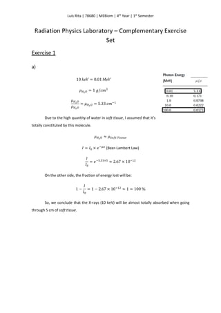
1. Luís Rita | 78680 | MEBiom | 4th
Year | 1st
Semester
Radiation Physics Laboratory – Complementary Exercise
Set
Exercise 1
a)
10 𝑘𝑒𝑉 = 0.01 𝑀𝑒𝑉
𝜌 𝐻2 𝑂 = 1 𝑔/𝑐𝑚3
𝜇 𝐻2 𝑂
𝜌 𝐻2 𝑂
= 𝜇 𝐻2 𝑂 = 5.33 𝑐𝑚−1
Due to the high quantity of water in soft tissue, I assumed that it’s
totally constituted by this molecule.
𝜇 𝐻2 𝑂 ≈ 𝜇 𝑆𝑜𝑓𝑡 𝑇𝑖𝑠𝑠𝑢𝑒
𝐼 = 𝐼0 × 𝑒−𝜇𝑥
(Beer-Lambert Law)
𝐼
𝐼0
= 𝑒−5.33×5
≈ 2.67 × 10−12
On the other side, the fraction of energy lost will be:
1 −
𝐼
𝐼0
= 1 − 2.67 × 10−12
≈ 1 = 100 %
So, we conclude that the X-rays (10 keV) will be almost totally absorbed when going
through 5 cm of soft tissue.

2. Luís Rita | 78680 | MEBiom | 4th
Year | 1st
Semester
b)
If we do just the same thing as before (now, for 100 MeV gamma rays), we realize that
the absorption won’t be as high as before. This was expected, just by observing Figure 1 (as high
is the photon energy, as low will be mass absorption coefficient).
𝐼
𝐼0
= 𝑒−0.0173×5
≈ 0.917
1 −
𝐼
𝐼0
= 1 − 0.917 = 0.083 = 8.3 %
Figure 1 – Mass absorption coefficient of photons in water.

3. Luís Rita | 78680 | MEBiom | 4th
Year | 1st
Semester
c)
Considering 1 beam of X-rays (10 keV) and another of gamma-rays (100 MeV) with the
same intensity, the energy lost by each one when focusing in soft tissue will be:
X-rays (0.01 MeV)
𝐸X−rays = 𝑁 × 0.01 × 1
Gamma-rays (100 MeV)
𝐸γ−rays = 𝑁 × 100 × 0.083
Finally, comparing the values of energy lost by these 2 types of radiation:
𝐸γ−rays
𝐸X−rays
=
𝑁 × 100 × 0.083
𝑁 × 0.01 × 1
= 830
In spite of the fraction of energy lost by gamma-rays being much lower than the one
associated to x-rays (previous questions), the first radiation is much more energetic, that’s why
we obtained
𝐸γ−rays
𝐸X−rays
= 830.

4. Luís Rita | 78680 | MEBiom | 4th
Year | 1st
Semester
d)
Starting by representing Photoelectric Effect, Compton Scattering and Pair Production
regions, we obtain Figure 2. Just by observing the graph, it’s evident that for x-ray radiations,
Photoelectric Effect will be predominant. And for energies around 100 MeV (gamma radiation),
Pair Production will be the observable phenomenon.
The main interaction between x-rays and matter will be by ionization and excitation. In
this specific case, between photons and Hydrogen/Oxygen atoms by ionization. In other words,
some atoms will release their electrons, in response to the incidence of 0.01 MeV photons.
Through these processes most of the radiation will be absorbed by the soft tissue.
For greater energies, we may find a phenomenon called Pair Production. As soon as each
photon is absorbed by the atoms, it’s expected that each one (atoms) will emit one electron and
one positron (conserving like these the initial momentum and energy). As Figure 2 shows, this
can only happen for photon energies greater than 𝐸 𝛾 = 2𝑚 𝑒 𝑐2
≈ 1.022 𝑀𝑒𝑉 > 100 𝑀𝑒𝑉.
Because each emitted particle will have to have at least 0.511 𝑀𝑒𝑉. This is verified, gamma-rays
have 100 𝑀𝑒𝑉. Concluding, gamma rays lose about 8 % of their energy, in 5 𝑐𝑚 of soft tissue,
this way.
Figure 2 – Photoelectric Effect, Compton Scattering and Pair Production regions.
X-rays
𝛾-rays

5. Luís Rita | 78680 | MEBiom | 4th
Year | 1st
Semester
Exercise 2
a)
𝑅 =
∆𝐸
𝐸
=
𝐹𝑊𝐻𝑀
𝐸
1.3325 − 1.1732 = 0.1593 𝑀𝑒𝑉 (Figure 3)
𝐹𝑊𝐻𝑀 < 0.1593
So, the maximum value of the energy resolution for the peak with the highest energy is
given by:
𝑅 × 𝐸 = 𝐹𝑊𝐻𝑀 < 0.1593
𝑅 <
0.1593
𝐸
=
0.1593
1.3325
= 0.12 or 𝑅(%) < 12 %
Figure 3 – Decay scheme of 60Co.

6. Luís Rita | 78680 | MEBiom | 4th
Year | 1st
Semester
b)
We can calculate a system resolution by to different ways:
 𝑅 =
∆𝐸
𝐸
(just as I did before);
 𝑅 =
∆𝑁
𝑁
(1)
Besides this, as we are working with a Poissonian distribution, the following expression is
also valid:
∆𝑁 = 2.35𝜎 = 2.35√𝑁 (2)
Joining expression (1) and (2):
𝑅 =
2.35√𝑁
𝑁
=
2.35
√𝑁
(3)
Now, calculating the number of photons emitted due to each transition, knowing that
the NaI scintillator emits one photon per 26 eV of energy deposited:
𝑁𝛾1
𝑒𝑚𝑖𝑡𝑡𝑒𝑑
=
1.3325 × 106
26
= 5.1 × 104
𝑝ℎ𝑜𝑡𝑜𝑛𝑠
𝑁𝛾2
𝑒𝑚𝑖𝑡𝑡𝑒𝑑
=
1.1732 × 106
26
= 4.5 × 104
𝑝ℎ𝑜𝑡𝑜𝑛𝑠
Photons with 1.3325 MeV were represented as 𝛾1 and with 1.1732 MeV as 𝛾2. Assuming
a constant detection efficiency of 5%:
𝑁𝛾1
𝑑𝑒𝑡𝑒𝑐𝑡𝑒𝑑
= 5.1 × 104
× 0.05 = 2.55 × 103
𝑝ℎ𝑜𝑡𝑜𝑛𝑠
𝑁𝛾2
𝑑𝑒𝑡𝑒𝑐𝑡𝑒𝑑
= 4.5 × 104
× 0.05 = 2.25 × 103
𝑝ℎ𝑜𝑡𝑜𝑛𝑠
Finally, using expression (3), it’s calculable the resolution for each peak:
𝑅 𝛾1(%) =
2.35
√2.55 × 103
× 100 = 4.65 % < 12 %
𝑅 𝛾2(%) =
2.35
√2.25 × 103
= 4.95 % < 12 %
As the resolution of both peaks, resulted from the decay of 60
Co, is lower than 12 %, we
conclude that the one created by photons 𝛾1 is distinguishable from the one created by 𝛾2.

7. Luís Rita | 78680 | MEBiom | 4th
Year | 1st
Semester
Exercise 3
a)
Knowing that the minimum energy loss of heavy particles in matter through excitation
and ionization processes corresponds to 𝛽𝛾 ≈ 3:
Kinetic Energy: 𝑇 = 𝐸 − 𝑚𝑐2
(4)
𝛾𝛽 = √(
𝐸
𝑚𝑐2
)
2
− 1
(𝛾𝛽)2
= (
𝐸
𝑚𝑐2
)
2
− 1 ⇔ 𝐸 = √((𝛾𝛽)2 + 1)(𝑚𝑐2)2 ⇔ 𝐸 = 𝑚𝑐2√(𝛾𝛽)2 + 1 (5)
Substituting 5 in 4, we obtain the kinetic energy expression depending only from the
mass of the particle:
𝑇 = 𝑚𝑐2√(𝛾𝛽)2 + 1 − 𝑚𝑐2
i. Muons (M = 105.7 MeV)
𝑇 = 105.7 × √10 − 105.7 = 228.55 𝑀𝑒𝑉
ii. Protons (M = 938.3 MeV)
𝑇 = 938.3 × √10 − 938.3 = 2.03 𝐺𝑒𝑉
iii. α particles (M = 3727.3 MeV)
𝑇 = 3727.3 × √10 − 3727.3 = 8.06 𝐺𝑒𝑉

8. Luís Rita | 78680 | MEBiom | 4th
Year | 1st
Semester
b)
Some relativistic initial identities that will be useful later on.
𝛾 =
𝐸
𝑚𝑐2
𝛽 = √1 −
1
𝛾2
= √1 −
1
𝐸2
𝑚2 𝑐4
𝛽2
= 1 −
1
𝐸2
𝑚2 𝑐4
⇔ 𝛽2
=
𝐸2
− 𝑚2
𝑐4
𝐸2
For low velocities (𝛽𝛾 < 3 − 3.5) Bethe-Bloch equation is, approximately:
−
𝑑𝐸
𝑑𝑥
≈ 𝑘
1
𝛽2
The average range for heavy charged particles is:
𝑅̅ = ∫
𝑑𝐸
−
𝑑𝐸
𝑑𝑥
𝑚𝑐2
𝐸0
= ∫
𝑑𝐸
𝑘
1
𝛽2
𝐸0
𝑚𝑐2 = ∫
𝑑𝐸
𝑘
1
𝐸2−𝑚2 𝑐4
𝐸2
𝐸0
𝑚𝑐2 =
1
𝑘
∫
𝐸2−𝑚2 𝑐4
𝐸2 𝑑𝐸
𝐸0
𝑚𝑐2 =
1
𝑘
[𝐸 +
𝑚2 𝑐4
𝐸
]
𝑚𝑐2
𝐸0
=
1
𝑘
(−
2𝑚𝑐2 𝐸0
𝐸0
+
𝐸0
2
𝐸0
+
𝑚2 𝑐4
𝐸0
) =
1
𝑘
(
𝑚2 𝑐4+𝐸0
2
−2𝑚𝑐2 𝐸0
𝐸0
) =
1
𝑘
(
(𝐸0−𝑚𝑐2)
2
𝐸0
) =
1
𝑘
𝑇0
2
𝐸0
(𝑐𝑚) ∎

9. Luís Rita | 78680 | MEBiom | 4th
Year | 1st
Semester
c)
i.
Before starting any calculations, it’s important to verify if alpha particles with a kinetic
energy of 3 MeV are moving quickly or slowly. Particularly, if 𝛽𝛾 < 3 − 3.5.
𝑀 = 3.73 × 109
𝑒𝑉
𝛾𝛽 = √(
𝑇 + 𝑚𝑐2
𝑀
)
2
− 1 = √(
3 × 106 + 3.73 × 109
3.73 × 109 )
2
− 1 = 0.04 ≪ 3
Again, assuming the soft tissue is totally made of water:
𝑍𝑆𝑜𝑓𝑡 𝑇𝑖𝑠𝑠𝑢𝑒 = 7.5 (presented in theoretical classes)
𝐴 𝑆𝑜𝑓𝑡 𝑇𝑖𝑠𝑠𝑢𝑒 = 𝐴 𝐻2 𝑂 = 16 + 1 + 1 = 18
𝑧 𝛼 𝑝𝑎𝑟𝑡𝑖𝑐𝑙𝑒 = +2
𝜌 𝑆𝑜𝑓𝑡 𝑇𝑖𝑠𝑠𝑢𝑒 = 𝜌 𝐻2 𝑂 = 1 𝑔𝑚/𝑐𝑚3
𝐼 𝐻2 𝑂 = 75 𝑒𝑉
𝑚 𝑒 𝑐2
= 511 𝑘𝑒𝑉
Substituting previous constants in k equation (provided in the Exercise set):
𝑘 = 0.1535 × 106
× 2 ×
𝑍
𝐴
𝑧2
𝜌 ln (
2𝑚 𝑒 𝑐2
𝐼
)
= 0.1535 × 106
× 2 ×
7.5
18
× (−2)2
× ln (
2 × 511 × 103
75
) = 4.871 𝑀𝑒𝑉
Finally, calculating the average crossing distance:
𝑅 =
1
𝑘
𝑇0
2
𝐸0
(6)
𝑅 =
1
4.871 × 106
(3 × 106
)2
3 × 106 + 3.73 × 109
= 4.95 × 10−4
𝑐𝑚

10. Luís Rita | 78680 | MEBiom | 4th
Year | 1st
Semester
ii.
Once again, before continuing we should verify if equation (6) is applicable. To do so, we
proceed just as before.
𝛾𝛽 = √(
𝑇 + 𝑚 𝑒 𝑐2
𝑚 𝑒 𝑐2 )
2
− 1 = √(
0.546 × 106 + 511 × 103
511 × 103 )
2
− 1 = 1.81 < 3
After verifying the low velocity condition, we can star calculating R.
𝑘 = 0.1535 × 106
× 2 ×
𝑍
𝐴
𝑧2
𝜌 ln (
2𝑚 𝑒 𝑐2
𝐼
)
= 0.1535 × 106
× 2 ×
7.5
18
× (−1)2
ln (
2 × 511 × 103
75
)
= 1.218 𝑀𝑒𝑉 (7)
The only difference between this case and the previous is the particle that was studied.
So, as expected the only value that was changed in equation (7) was the charge of the particle.
𝑅 =
1
𝑘
𝑇0
2
𝐸0
=
1
1.218 × 106
(0.546 × 106
)2
0.546 × 106 + 511 × 103
= 0.23 𝑐𝑚
The average range of the most energetic electrons emitted from 90
Sr is 0.23 cm.
Note: to obtain the value from the most energetic electrons emitted from 90
Sr, I
searched in Wikipedia (https://en.wikipedia.org/wiki/Strontium-90).

11. Luís Rita | 78680 | MEBiom | 4th
Year | 1st
Semester
Exercise 4
Like in exercise 3, it will be assumed that there aren’t radiative losses. First of all, it is
necessary to verify if we are in the presence of a case of low velocities. To do that, we compare
the product 𝛽𝛾 with the limit of the region of small velocities 𝛽𝛾 = 3.
𝑇 𝑚𝑎𝑥 ≡ 𝑄 = 0.764 𝑀𝑒𝑉 (https://en.wikipedia.org/wiki/Thallium)
𝛾𝛽 = √(
𝑇 𝑚𝑎𝑥 + 𝑚 𝑒 𝑐2
𝑚 𝑒 𝑐2 )
2
− 1 = √(
0.764 × 106 + 511 × 103
511 × 103 )
2
− 1 = 2.29 < 3
Once, I calculated 𝛾𝛽 with 𝑇 𝑚𝑎𝑥, we will certainly remain in the valid region after
calculating the kinetic energy later.
Useful data:
𝑍
𝐴
= 0.5 (as studied in the theoretical classes, it’s a valid approximation for small atomic
numbers)
𝜌 𝑝𝑜𝑙𝑦𝑒𝑡ℎ𝑦𝑙𝑒𝑛𝑒 = 0.935 𝑔𝑚/𝑐𝑚3
(https://en.wikipedia.org/wiki/Polyethylene)
𝐼 𝑝𝑜𝑙𝑦𝑒𝑡ℎ𝑦𝑙𝑒𝑛𝑒 = 57.4 𝑒𝑉 (http://physics.nist.gov/cgi-
bin/Star/compos.pl?mode=text&refer=ap&matno=221)
𝑘 = 0.1535 × 106
× 2 ×
𝑍
𝐴
𝑧2
𝜌 ln (
2𝑚 𝑒 𝑐2
𝐼
)
= 0.1535 × 106
× 2 × 0.5 × (−1)2
0.935 ln (
2 × 511 × 103
57.4
)
= 1.405 𝑀𝑒𝑉 (7)
Now, we are able to calculate the kinetic energy related to an average crossing of 0.15
cm.
𝑅 =
1
𝑘
𝑇𝑒
2
𝑇𝑒+𝑚 𝑒 𝑐2 ⇔ 𝑘𝑅𝑇𝑒 + 𝑘𝑅𝑚 𝑒 𝑐2
= 𝑇𝑒
2
⇔ 𝑇𝑒 = 0.450 𝑀𝑒𝑉 (other solution doesn’t
have physical meaning (<0))
Finally, to determine shielding efficiency, we just have to calculate the ratio between
the number of electron with a kinetic energy until 450 keV and number of particles with energies
until the end point of the spectrum.

12. Luís Rita | 78680 | MEBiom | 4th
Year | 1st
Semester
Number of shielded electrons:
∫ 𝑁(𝑇𝑒)𝑑𝑇𝑒
𝑇𝑒
0
= ∫ 𝑐𝑜𝑛𝑠𝑡√𝑇𝑒
2 + 2𝑇𝑒 𝑚 𝑒 𝑐2(𝑄 − 𝑇𝑒)2
(𝑇𝑒 + 𝑚 𝑒 𝑐2
)𝑑𝑇𝑒
450×103
0
= 𝑐𝑜𝑛𝑠𝑡 × 4.22 × 1028
𝑐𝑜𝑢𝑛𝑡𝑠
Total number of electrons:
∫ 𝑁(𝑇𝑒)𝑑𝑇𝑒
𝑄
0
= ∫ 𝑐𝑜𝑛𝑠𝑡√𝑇𝑒
2 + 2𝑇𝑒 𝑚 𝑒 𝑐2(𝑄 − 𝑇𝑒)2
(𝑇𝑒 + 𝑚 𝑒 𝑐2
)𝑑𝑇𝑒
764×103
0
= 𝑐𝑜𝑛𝑠𝑡 × 5.19 × 1028
𝑐𝑜𝑢𝑛𝑡𝑠
Both integrals were calculated numerically using a software present in:
http://www.integral-calculator.com/.
Finally, shielding efficiency will be:
∫ 𝑁(𝑇𝑒)𝑑𝑇𝑒
𝑇𝑒
0
∫ 𝑁(𝑇𝑒)𝑑𝑇𝑒
𝑄
0
× 100 =
𝑐𝑜𝑛𝑠𝑡 × 4.22 × 1028
𝑐𝑜𝑛𝑠𝑡 × 5.19 × 1028
× 100 = 81.3 %

13. Luís Rita | 78680 | MEBiom | 4th
Year | 1st
Semester
Exercise 5
a)
The ratio
𝑁𝑢𝑚𝑏𝑒𝑟 𝑝𝑎𝑟𝑡𝑖𝑐𝑙𝑒𝑠 𝑟𝑒𝑎𝑐ℎ𝑖𝑛𝑔 𝑑𝑒𝑡𝑒𝑐𝑡𝑜𝑟
𝑁𝑢𝑚𝑏𝑒𝑟 𝑝𝑎𝑟𝑡𝑖𝑐𝑙𝑒𝑠 𝑒𝑚𝑖𝑡𝑡𝑒𝑑 𝑏𝑦 𝑡ℎ𝑒 𝑠𝑜𝑢𝑟𝑐𝑒
can be obtained using the following
expression:
𝑅 =
Ω
4𝜋
Ω corresponds to the solid angle occupied by the detector and 4𝜋 𝑠𝑟 is the solid angle
of a sphere. It only makes sense to use this formula because the source is isotropic.
Exact definition Ω
𝑐𝑜𝑠𝜃 𝑚𝑎𝑥 =
𝑑
√𝑑2 + 𝑎2
=
1
√1 + (
𝑎
𝑑
)
2
Ω 𝑒𝑥𝑎𝑐𝑡 = ∫ dΩ = 2𝜋(1 − 𝑐𝑜𝑠𝜃 𝑚𝑎𝑥) = 2𝜋
(
1 −
1
√1 + (
𝑎
𝑑
)
2
)
= 0.0312 𝑠𝑟
𝑅 𝑒𝑥𝑎𝑐𝑡 =
0.0312
4𝜋
= 0.00248
For reasons of simplicity and because it’s 2 orders of magnitude below 15.00 cm, the
uncertainty in d distance was neglected.
Approximation 𝑎 ≪ 𝑑
Ω 𝑎𝑝𝑝𝑟𝑜𝑥 = 𝜋
𝑎2
𝑑2
= 0.0314 𝑠𝑟
𝑅 𝑎𝑝𝑝𝑟𝑜𝑥 =
0.0314
4𝜋
= 0.0025
Previous calculations confirm that the approximation 𝑎 ≪ 𝑑 is valid. 𝑅 𝑒𝑥𝑎𝑐𝑡 and 𝑅 𝑎𝑝𝑝𝑟𝑜𝑥
are almost the same.
𝑎 = 1.5 𝑐𝑚
𝑑 = 15.00 ± 0.05 𝑐𝑚

14. Luís Rita | 78680 | MEBiom | 4th
Year | 1st
Semester
b)
This experiment is described by a Poisson distribution. So, the relative error in the
number of counts (n) is given by
1
√ 𝑛
. Consequently, if we pretend to obtain a statistical
uncertainty below 1%,
1
√ 𝑛
< 0.01 ⇔ 𝑛 > 10 000 𝑒𝑙𝑒𝑐𝑡𝑟𝑜𝑛𝑠 should be detected.
Assuming the electrons don’t interact with the air and the detector’s efficiency is 100%,
it’s possible to calculate the number of these particles that should emitted by the source:
𝑁 =
10 000
0.00248
= 4.03 × 106
𝑒𝑚𝑖𝑡𝑡𝑒𝑑 𝑒𝑙𝑒𝑐𝑡𝑜𝑛𝑠

15. Luís Rita | 78680 | MEBiom | 4th
Year | 1st
Semester
c)
i.
We know that the detector acquired for 100 seconds a bunch of particles at a count rate
of 400 cnts/s. It’s also known that from those 400 cnts/s, it’s included a background rate of 1.0 ±
0.1 cnts/s. Goal: calculate the count rate of particles emitted by the source (and detected) and
its statistical error.
Starting by calculating the uncertainty related to the overall count rate (Source +
Background):
Δ𝐶𝑅 𝑆+𝐵 = √(Δ𝑛)2 (
1
𝑡
)
2
+ (Δ𝑡)2 (
1
𝑡2
)
2
= √
40000
10000
= 2 𝑐𝑛𝑡𝑠/𝑠
𝐶𝑅 𝑆+𝐵 = 400 ± 2 𝑐𝑛𝑡𝑠/𝑠
Δ𝑡 ≈ 0 because it’s much lower than Δ𝑛.
Finally, it was asked us to calculate the number of counts (only from the source) and
related uncertainty.
Δ𝐶𝑅 𝑆 = √(Δ𝐶𝑅 𝑆+𝐵)2 + (𝐶𝑅 𝐵)2 = √(2)2 + (0.1)2 = 2.0025 ≈ 2 𝑐𝑛𝑡𝑠/𝑠
𝐶𝑅 𝑆 = 399 ± 2 𝑐𝑛𝑡𝑠/𝑠

16. Luís Rita | 78680 | MEBiom | 4th
Year | 1st
Semester
ii.
The relative error obtained before for the total number counts performed in c) is:
∆𝐶 =
1
√40 000
= 0.005 = 0.5 %
So, if we want to obtain the same relative error but now for the background counting,
the same number of detections must be performed.
𝐶𝑅 =
𝑁𝑢𝑚𝑏𝑒𝑟 𝑜𝑓 𝐶𝑜𝑢𝑛𝑡𝑠
∆𝑡
⇔ ∆𝑡 = 40 000 𝑠 ≈ 11 ℎ𝑜𝑢𝑟𝑠

17. Luís Rita | 78680 | MEBiom | 4th
Year | 1st
Semester
d)
Starting by converting half-life and the 204
Tl source age to seconds, we get:
𝑇1
2
= 3.78 × 365.25 × 24 × 3600 = 1.192 × 108
𝑠
∆𝑇 = 10 × 365.25 × 24 × 3600 = 3.156 × 108
𝑠
Now, using the exponential decay formula, we calculate 𝜆 coefficient.
𝐴 = 𝐴0 𝑒−𝜆𝑡
⇔
𝐴0
2
= 𝐴0 𝑒−𝜆×1.192×108
⇔ 𝜆 = 5.815 × 10−9
𝑠−1
The activity after 10 years will be:
𝐴 = 37 × 103
× 𝑒−5.815×10−9×3.156×108
= 5904.44 𝐵𝑞
1 𝜇𝐶𝑖 = 37 × 103
𝐵𝑞
Finally, assuming that the efficiency of the detector is 100 %, the count rate will be:
𝐶𝑅 = 5904.44 ×
0.0312
4𝜋
= 14.6 𝑐𝑛𝑡𝑠/𝑠