SlideShare a Scribd company logo
1 of 35
Download to read offline
Taguchi Techniques
1 MGM‟s Jawaharlal Nehru Engineering College
INDEX
Chapter
Number
Chapter Particulars Page Number
Literature Review 2
1 Introduction 4
1.1 Definitions of Quality 5
1.2 Taguchi Definition of Quality 6
2 Taguchi Loss Function 7
2.1 Taguchi‟s Quality Philosophy 8
3 Objective of Taguchi Methods 11
3.1 Eight steps in Taguchi Methodology 11
4 Quadratic Loss Function 12
4.1 Variation of Quadratic Loss Function 14
5 Signal to Noise Ratio 16
6 Case Study I 18
7 Orthogonal Arrays 25
8 Case Study II 28
9 Conclusion and Future Scope 33
9.1 Conclusion 33
9.2 Future Scope 33
10 References 34
Taguchi Techniques
2 MGM‟s Jawaharlal Nehru Engineering College
LITERATURE REVIEW
Paper
No.
Book / Research Paper Title Author Year
1. Taguchi Techniques for Quality
Engineering.
Phillip J. Ross 2005
2.
Design and Analysis of
Experiments.
Douglas C. Montgomery 2001
3.
Application of Taguchi method in
the optimization of End Milling
parameters
J. A. Ghani
I. A. Choudhary
H. H. Hassan
2003
4.
Optimisation of Deep Drilling
Process Parameters of AISI 321
Steek using Taguchi Method
Arshad Noor Siddiqueee
Zahid A. Khan
Mukesh Kumar
2014
5. Robust Design
K. Sudhakar
P. M. Mujumdar 2002
6.
The Taguchi Methods of quality
control examined:
with reference to Sundstrand-Sauer
Cheryl Lynn Moller-Wong 1988
Taguchi Techniques
3 MGM‟s Jawaharlal Nehru Engineering College
TABLE & GRAPH INDEX
Table/ Graph
Number
Title of Table/ Graph Page Number
G1 Traditional Quality Definition 6
G2 Taguchi Quality Definition 6
G3 Traditional Interpretation of Specification 8
G4 Time Temperature Relationship 10
G5 Nominal the better 14
G6 Smaller the better 14
G7 Larger the better 15
G8 Asymmetric 15
T1 Comparison between Signal to Noise Ratios 17
G9 Outer Diameter Histogram 18
G10 Outer Diameter Loss Function 19
T2 Cost of part versus outer Diameter 20
G11 Distribution due to tool wear 22
G12 Cost comparison 23
T3 Orthogonal Array 26
T4 Orthogonal Arrays 27
T5 23
Factorial Design 27
T6 24
Factorial Design 27
T7 Interaction Columns of an Orthogonal Array 29
Taguchi Techniques
4 MGM‟s Jawaharlal Nehru Engineering College
1. INTRODUCTION
When Japan began its reconstruction efforts after World War II, Japan faced an acute
shortage of good quality raw material, high quality manufacturing equipment and skilled
engineers. The challenge was to produce high quality products and continue to improve
quality product under these circumstances.
The task of developing a methodology to meet the challenge was assigned to Dr. Genichi
Taguchi, who at that time was manager in charge of developing certain
telecommunication products at the electrical communication laboratories (ECL) of
Nippon Telecom and Telegraph Company (NTT).
Through his research in the early 1960‟s, Dr Taguchi developed the foundation of
Orthogonal Arrays and Robust design and validated his basics philosophies by applying
them in the development of many products. He developed the concept of the Quality Loss
Function in the 1970‟s. He also published the third and most current edition of his book
on experimental designs. Genichi Taguchi made many important contributions during his
lifetime in the field of quality control. The term Taguchi Methods is coined after him. Dr
Taguchi received the individual DEMING AWARD in 1962, which is one of the highest
recognition in the quality field.
When the need is to have a process so robust that the process may not stay always within
the specification but needs to stay centred at the target, Taguchi‟s Techniques are very
useful. The underlying belief in this process is that every time a process moves away from
the target there is loss to customer even if the process is within the specifications. This
method focuses not only on the controllable factors as in conventional design of
experiments but also considering the noise factors.
Taguchi Techniques
5 MGM‟s Jawaharlal Nehru Engineering College
1.1 TRADITIONAL DEFINITION OF QUALITY
The term, „Quality‟ was defined in the following way:
 “Fitness for use”
 Dr. Juran (1964)
 The leading promoter of the “zero defects” concept and author of Quality is Free
(1979) defines quality as” Conformance to requirements.
 Philips Crosby
 Quality should be aimed at needs of consumer, present and future.
 Dr. Deming
 The totality of features and characteristics of a product or service that bears on its
ability to satisfy given needs.
 The American Society for Quality Control (1983)
 The aggregate of properties of a product determining its ability to satisfy the needs it
was built to satisfy.
 (Russian Encyclopedia)
 The totality of features and characteristics of a product and service that bear on its
ability to satisfy a given need.
 (European Organization for Quality Control Glossary 1981)
Although these definitions are all different, some common threads run through them:
 Quality is a measure of the extent to which customer requirements and
expectations are satisfied.
 Quality is not static, since customer expectation can change.

Quality involves developing product or service specifications and standards to meet
customer needs (quality of design) and then manufacturing products or providing services
which satisfy those specifications and standards (quality of conformance). It is important
to note that the above quality definitions which are before 1950‟s does not refer to grade
or features. For example Honda Car has more features and is generally considered to be a
higher grade car than Maruti. But it does not mean that it is of better quality. A couple
with two children may find that a Maruti does a much better job of meeting their
requirements in terms of case of loading and unloading ,comfort when the entire family is
in the car, gas mileage, maintenance, and of course ,basic cost of vehicle.
Taguchi Techniques
6 MGM‟s Jawaharlal Nehru Engineering College
1.2 TAGUCHI DEFINITION OF QUALITY
Traditional Definition:
The more traditional "Goalpost"
mentality of what is considered good
quality says that a product is either good
or it isn't, depending or whether or not it
is within the specification range
(between the lower and upper
specification limits -- the goalposts).
With this approach, the specification
range is more important than the nominal
(target) value. But, is the product as good
as it can be, or should be, just because it
is within specification.
G1
Taguchi Definition:
Taguchi says no to above definition. He
define the „quality‟ as deviation from on-
target performance. According to him,
quality of a manufactured product is total
loss generated by that product to society
from the time it is shipped. Financial loss
or Quality loss.
G2
Taguchi Techniques
7 MGM‟s Jawaharlal Nehru Engineering College
2. TAGUCHI LOSS FUNCTION
Taguchi loss function recognizes the customer‟s desire to have products that are more
consistent, part to part, and a producer‟s desire to make low cost products.
Genichi Taguchi has an unusual definition for product quality: “Quality is the loss a
product causes to society after being shipped, other than any losses caused by its intrinsic
functions.” By “loss” Taguchi refers to the following two categories.
• Loss caused by variability of function.
• Loss caused by harmful side effects.
An example of loss caused by variability of function would be an automobile that does
not start in cold weather. The car‟s owner would suffer a loss if he or she had to pay some
to start a car. The car owner‟s employer loses the services of the employee who is now
late for work. An example of a loss caused by a harmful side effect would be frost (cold)
suffered by the owner of the car which would not start.
An unacceptable product which is scrapped or rework prior to shipment is viewed by
Taguchi as a cost to the company but not a quality loss.
Taguchi suggests defining the function as follows:
Loss (y) = 𝑘 𝑦 − 𝑚 2
Where, k = A / 𝑑2
And
A = the cost of corrective action necessary to change the process
d = the value of the process
m = the target value of the process characteristic
y = the measurement of the unit in question
k = the loss coefficient
Loss (y) = the incremental loss
Taguchi Techniques
8 MGM‟s Jawaharlal Nehru Engineering College
G3: Traditional interpretation of specification.
2.1 TAGUCHI’S QUALITY PHILOSOPHY
Genichi Taguchi‟s impact on the word quality scene has been far- reaching. His quality
engineering system has been used successfully by many companies in Japan and
elsewhere. He stresses the importance of designing quality into product into processes,
rather than depending on the more traditional tools of on-line quality control. Taguchi‟s
approach differs from that of other leading quality gurus in that he focuses more on the
engineering aspects of quality rather than on management philosophy of statistics. Also,
Dr. Taguchi uses experimental design primarily as a tool to make products more robust-
to make them less sensitive to noise factors. That is, he views experimental design as a
tool for reducing the effects of variation on product and process quality characteristics.
Earlier applications of experimental design focused more on optimizing average product
performance characteristics without considering effects on variations. Taguchi‟s quality
philosophy seven basic elements:
Taguchi Techniques
9 MGM‟s Jawaharlal Nehru Engineering College
1. An important dimension of the quality of a manufactured product is the total loss
generated by product to society. At a time when the BOTTOM LINE appears to be the
driving force for so many organizations, it seems strange to see “loss to society” as part of
product quality.
2. In a competitive economy, continuous quality improvement and cost reduction are
necessary for staying in business. This is hard lesson to learn. Masaaki Imai (1986) argues
very persuasively that the principal difference between Japanese and American
management is that American companies look to new technologies and innovation as the
major route to improvement, while Japanese companies focus more on “Kaizen” means
gradual improvement in everything they do. Taguchi stresses use of experimental designs
in parameter design as a way of reducing quality costs. He identifies three types quality
costs: R & D costs, manufacturing costs, and operating costs. All three costs can be
reduced through use of suitable experimental designs.
3. A continues quality improvement program includes continuous reduction in the
variation of product performance characteristics about their target values. Again Kaizen.
But with the focus on product and process variability this does not fit the mould of quality
being of conformance to specification.
4. The customer‟s loss due to a product‟s performance variation is often
approximately proportional to the square of the deviation of the performance
characteristic from its target value. This concept of a quadratic loss function, says that any
deviation from target results in some loss of the customer, but that large deviations from
target result in severe losses.
5. The final quality and cost of manufactured product are determined to a large
extent by the engineering designs of the product and its manufacturing process. This is so
simple, and so true. The future belongs to companies, which, once they understand the
variability‟s of their manufacturing processes using statistical process control, move their
quality improvement efforts upstream to product and process design.
Taguchi Techniques
10 MGM‟s Jawaharlal Nehru Engineering College
6. A product (or process) performance variation can be reduced by exploiting the
nonlinear effects of the product (or process) parameters on the performance
characteristics. This is an important statement because its gets to the heart of off-line QC.
Instead of trying to tighten speciation beyond a process capability, perhaps a change in
design can allow specifications to be loosened. As an example, suppose that in a heating
process the tolerance on temperature is a function of the heating time in the oven. The
tolerance relationship is represents by the band in given figure. For example : If a process
specification says the heating process is to last 4.5 minutes, then the temperature must be
held between 354.0 degrees and 355.0 degrees, a tolerance interval 1.0 degrees wide.
Perhaps the oven cannot hold this tight a tolerance. One solution would be spending a lot
of money on a new oven and new controls. Other possibility would be to change the time
for the heating process to, say, 3.5 minutes. Then the temperature would need to be held
to between 358.0 and 360.6 degrees an interval of width 2.6 degrees. If the oven could
hold this tolerance, the most economical decision might be to adjust the specifications.
This would make the process less sensitive to variation in oven temperature.
G4: Time Temperature relationship
7. Statistically designed experiments can be used to identify the settings of product
parameters that reduce performance variations. And hence improve quality, productivity,
performance, reliability, and profits, statistically designed experiments will be the
strategic quality weapon of the 1990‟s.
Taguchi Techniques
11 MGM‟s Jawaharlal Nehru Engineering College
3. OBJECTIVE OF TAGUCHI METHODS
The objective of Taguchi‟s efforts is process and product-design improvement through the
identifications of easily controllable factors and their settings, which minimize the
variation in product response while keeping the mean response on target. By setting those
factors at their optimal levels, the product can be made robust to changes in operating and
environmental conditions. Thus, more stable and higher-quality products can be obtained,
and this is achieved during Taguchi‟ parameter-design stage by removing the bad effect of
the cause rather than the cause of the bad effect. Furthermore, since the method is applied
in a systematic way at a pre-production stage (off-line), it can greatly reduce the number
of time-consuming tests needed to determine cost-effective process conditions, thus
saving in costs and wasted products.
3.1 EIGHT-STEPS IN TAGUCHI METHODOLOGY
1. Identify the main function, side effects and failure mode.
2. Identify the noise factor, testing condition and quality characteristics.
3. Identify the objective function to be optimized.
4. Identify the control factor and their levels.
5. Select the Orthogonal Array, Matrix experiments.
6. Conduct the Matrix equipment.
7. Analyze the data; predict the optimum levels and performance.
8. Perform the verification experiment and plan the failure action.
Taguchi Techniques
12 MGM‟s Jawaharlal Nehru Engineering College
4. QUADRATIC LOSS FUNCTION
When an objective characteristic y deviates from its target value m, some financial loss
will occur. Therefore, the financial loss, sometimes referred to simply as quality loss or
used as an expression of quality level, can be assumed to be a function of y, which we
shall designate L(y), When y meets the target m, the of L(y) will be at minimum;
generally, the financial loss can be assumed to be zero under this ideal condition:
L (m) = 0 ……………… Equation 2.1
Since the financial loss is at a minimum at the point, the first derivative of the loss
function with respect to y at this point should also be zero. Therefore, one obtains the
following equation:
L΄ (m) = 0 …………….. Equation 2.2
If one expand the loss function L(y) through a Taylor series expansion around the target
value m and takes Equations (2.1) and (2.2) into consideration, one will get the following
equation:
L(y) = L(m) + L΄ (m)(y-m)/1!+L΄΄(m)(y-m) ²/2!+ ……………
=L΄΄(y-m)²/2! +………
Result is obtained because the constant term L(m) and the first derivative term L‟(m) are
both zero. In addition, the third order and higher order term are assumed to be negligible.
Thus, one can express the loss function as a squared term multiplied by constant k:
L(y) =k(y-m)² …………… Equation 2.3
Taguchi Techniques
13 MGM‟s Jawaharlal Nehru Engineering College
When the deviation of the object characteristic from the target value increases, the
corresponding quality loss will also increase. When magnitude of deviation is outside of
the tolerance specifications, this product should be considered defective.
Let the cost due to defective product be A and the corresponding magnitude of the
deviation from the target value be. Taking into right hand side of Equation (2.3), one can
determine the value for constant k by following Equation:
k=cost of defective product / (tolerance)²
Consider the visitor to the BHEL Heavy Electric Equipment Company in India who was
told, “In our company, only one unit of product needs to be made for our nuclear power
plant. In fact, it is not really necessary for us to make another unit of product. Since the
sample size is only one, the variance is zero. Consequently, the quality loss is zero and it
is not really necessary for us to apply statistical approaches to reduce the variance of our
product.”
However, the quality loss function [L = k(y – m) ²] is defined as the mean square
deviation of objective characteristics from their target value, not the variance of products.
Therefore, even when only one product is made, the corresponding quality loss can still be
calculated by Equation (2.3). Generally, the mean square deviation of objective
characteristics from their target values can be applied to estimate the mean value of
quality loss in Equation (2.3). One can calculate the mean square deviation from target σ²
(σ² in this equation is not variance) by the following equation (the term σ² is also called
the mean square error or the variance of products):
Taguchi Techniques
14 MGM‟s Jawaharlal Nehru Engineering College
4.1 VARIATION OF THE QUADRATIC LOSS FUNCTION
Nominal the best type:
Whenever the quality characteristic y has a finite target value, usually nonzero, and the
quality loss is symmetric on the either side of the target, such quality characteristic called
nominal-the-best type. This is given by equation
L(y) =k(y-m) ²
G5
Colour density of a television set and the output voltage of a power supply circuit are
examples of the nominal-the-best type quality characteristic.
Smaller-the-better type:
Some characteristic, such as radiation leakage from a microwave oven, can never take
negative values. Also, their ideal value is equal to zero, and as their value increases, the
performance becomes progressively worse. Such characteristic are called smaller-the-
better type quality characteristics. The response time of a computer, leakage current in
electronic circuits, and pollution from an automobile are additional examples of this type
of characteristic. The quality loss in such situation can be approximated by the following
function, which is obtain from equation by substituting m = 0
L(y) =ky²
This is one side loss function because y cannot take negative values.
G6
Taguchi Techniques
15 MGM‟s Jawaharlal Nehru Engineering College
Larger-the-better type:
Some characteristics, such as the bond strength of adhesives, also do not take negative
values. But, zero is there worst value, and as their value becomes larger, the performance
becomes progressively better-that is, the quality loss becomes progressively smaller. Their
ideal value is infinity and at that point the loss is zero. Such characteristics are called
larger-the-better type characteristics. It is clear that the reciprocal of such a characteristics
has the same qualitative behaviour as a smaller-the-better type characteristic. Thus we
approximate the loss function for a larger-the-better type characteristic by substituting 1/y
for y in
L(y) = k [1/y²]
G7
Asymmetric loss function:
In certain situations, deviation of the quality characteristic in one direction is much more
harmful than in the other direction. In such cases, one can use a different coefficient k for
the two directions. Thus, the quality loss would be approximated by the following
asymmetric loss function:
k ( y – m ) ²,y > m
L(y) = k(y-m) ², y ≤ m
G8
Taguchi Techniques
16 MGM‟s Jawaharlal Nehru Engineering College
5. SIGNAL TO NOISE RATIO
In Taguchi designs, a measure of robustness used to identify control factors that reduce
variability in a product or process by minimizing the effects of uncontrollable factors
(noise factors). Control factors are those design and process parameters that can be
controlled. Noise factors cannot be controlled during production or product use, but can
be controlled during experimentation. In a Taguchi designed experiment, you manipulate
noise factors to force variability to occur and from the results, identify optimal control
factor settings that make the process or product robust, or resistant to variation from the
noise factors. Higher values of the signal-to-noise ratio (S/N) identify control factor
settings that minimize the effects of the noise factors.
Taguchi experiments often use a 2-step optimization process. In step 1 use the signal-to-
noise ratio to identify those control factors that reduce variability. In step 2, identify
control factors that move the mean to target and have a small or no effect on the signal-to-
noise ratio.
The signal-to-noise ratio measures how the response varies relative to the nominal or
target value under different noise conditions. You can choose from different signal-to-
noise ratios, depending on the goal of your experiment. For static designs, Minitab offers
four signal-to-noise ratios as shown in figure.
The Nominal is Best (default) signal-to-noise ratio is useful for analyzing or identifying
scaling factors, which are factors in which the mean and standard deviation vary
proportionally. Scaling factors can be used to adjust the mean on target without affecting
signal-to-noise ratios.
Taguchi Techniques
17 MGM‟s Jawaharlal Nehru Engineering College
T1: Comparison between Signal to Noise Ratios
Taguchi Techniques
18 MGM‟s Jawaharlal Nehru Engineering College
6. CASE STUDY I
Tool Wear in a Process
This case study is intended to show cost-oriented approach to quality control. With a very
capable process goalpost philosophy allows tool wear to produce parts which vary from
one specification limit to other. The lost function economically justifies different quality
control approach. An important aspect of product and process quality is the relative width
of the distribution and the specification limits of the product. If the distribution is
narrower than the specification limits of the products, then it is possible to make all or
nearly all parts. All of this is desirable from goalpost point of view.
A typical tolerance of machined part is to be +- 0.25mm. A process that would be very
capable with respect to this tolerance would be modelled as shown in figure.
G9: Outer Diameter Histogram.
The Taguchi loss function quantifies the variability present in a process. If a part reaches
the end of the manufacturing line with diameter exceeding the upper or lower limit, the
part should be scrapped at $4.00. The scrap cost is one aspect of loss to society.
Using the cost as a reference value, a loss function can be constructed as shown in figure.
Taguchi uses the mathematical equation to model this picture of cost v/s outer diameter.
Loss (y) = 𝑘 𝑦 − 𝑚 2
Taguchi Techniques
19 MGM‟s Jawaharlal Nehru Engineering College
G10: Outer Diameter Loss Function.
This equation, L is the loss associated with a diameter value y, m is the nominal value of
specification, and value of k is a constant depending upon the cost at the specification
limits and the width of specification.
L = 𝑘 𝑦 − 𝑚 2
$4.00 = k 𝐿𝑆𝐿 – 𝑚
2
The lower specification limit (LSL) is substituted into equation, which is where the $4.00
loss is incurred. The upper specification limit also could be used for this calculation.
Solving for k,
𝑘 =
$4.00
𝐿𝑆𝐿 – 𝑚 2
𝑘 =
$4.00
−0.010 – 0.0 2
k = $40,000 per sq in.
L = 40,000 𝑦 − 0.0 2
Now the loss associated with any part can be computed depending on the value of its
diameter.
Taguchi Techniques
20 MGM‟s Jawaharlal Nehru Engineering College
For instance, a part with diameter of + 0.003 in (+ 0.08 mm) costs
L = 40,000 0.003 − 0.0 2
L = $ 0.36
This is the loss per unit for each part shipped with an outer diameter of +0.003 in.
Similarly for a part diameter of -0.002 in which are 11 quantities in number the cost
incurred would be,
L ( - 0.002 ) = $ 40,000 −0.002 − 0.0 2
= $ 0.16 x 11
= $1.76
𝐿 =
$10.56
100 𝑃𝑎𝑟𝑡𝑠
$0.11 per part
T2: Cost of part versus outer Diameter
Taguchi Techniques
21 MGM‟s Jawaharlal Nehru Engineering College
A second method of estimating average loss per part entails using the loss equation in a
slightly modified form. Mathematically, this calculation is equivalent to using the average
value of the 𝑦 − 𝑚 2
portion of the loss equation.
𝐿 =
𝑘[ 𝑦1 − 𝑚 2
+ 𝑦2 − 𝑚 2
+ … + 𝑦𝑛 − 𝑚 2
]
𝑁
Where, N: number of parts sampled
If all the values of (y – m) values are squared, added together and divided by the number
of items, then the result is desired value. For a large number of parts, the average loss per
part is equivalent to
𝐿 = 𝑘 𝑆2
+ 𝑦 − 𝑚 2
𝑆2
: Variance around the average.
𝑦 : Average value of y for the group.
𝑦 − 𝑚 : Offset of the group average.
𝑆2
= 2.64 x 10⁻⁶
𝑖𝑛2
𝑦 = 0.0
𝐿 = 𝑘 𝑆2
+ 𝑦 − 𝑚 2
𝐿 = 40,000 2.64 𝑋 10−6
+ 0.0 − 0.0 2
𝐿1 = $ 0.11 per part
This second method uses the general loss function for a nominal is best situation.
Taguchi Techniques
22 MGM‟s Jawaharlal Nehru Engineering College
This example demonstrates the loss associated with a distribution that has a very good
process capability ratio and is centrally located on the target value of 0.0 in. Traditional
quality control would cause a situation where there would be a variation in size.
The loss function uses the average and variance for a group of parts to calculate loss. For
a group of parts where the distribution average is continually increasing, the variance is
G11: Distribution due to tool wear
𝑆 𝑅𝑒𝑠𝑢𝑙𝑡𝑎𝑛𝑡
2
= 𝑆 𝑂𝑟𝑖𝑔𝑖𝑛𝑎𝑙
2
+
𝑊2
12
Where W is the width of tool wear allowed.
𝑆 𝑂
2
= 2.64 𝑥 10−6
𝑖𝑛2
W = 0.010 in
𝑆 𝑅
2
= 2.64 𝑥 10−6
+
0.0102
12
= 1.10 x 10⁻⁵
Taguchi Techniques
23 MGM‟s Jawaharlal Nehru Engineering College
The loss per part is then,
𝐿 = 𝑘 𝑆2
+ 𝑦 − 𝑚 2
𝐿2 = $ 40,000 1.10 𝑥 10−5
+ 0 − 0 2
= $ 0.44
It is clear that, Loss of centred distribution is less than that of a distribution which
traverses the specification range.
L1 < L2
But to obtain a low loss the machine would have to be adjusted after each part. For the
second situation, the machine would not have to be adjusted nearly as often. Therefore,
there must be compromise between loss function and adjustment costs.
Ca = adjustment cost per part for N parts
La = k
𝑊2
12
N = number of parts made since last adjustment
N = W / R
R = wear rate of tool
G12: Cost comparison
Taguchi Techniques
24 MGM‟s Jawaharlal Nehru Engineering College
Ca = R x (total m/c adjustment cost / W)
The true optimisation cost is at 0.005 in tool wear span, but the additional loss of going up
to 0.006 in total span is very minimal ($ 0.003), which is beyond the accuracy of the loss
function. Adjustment width is 0.006 in, i.e. + 0.003 to –0.003 to get a centred nominal
value of 0.0 in as the optimum adjustment interval depends upon the scrap loss of a part.
This case study shows the economic penalty of allowing excessive variation in a product
or a process. Taguchi uses a very comprehensive economic approach to on-line
production quality control.
Taguchi Techniques
25 MGM‟s Jawaharlal Nehru Engineering College
7. ORTHOGONAL ARRAYS
An Array‟s name indicates the number of rows and column it has, and also the number of
levels in each of the column. Thus the array L4 (2³) has four rows and three 2-level
column. Historically, related methods was developed for agriculture, largely in UK,
around the Second World War, Sir R.A.Fisher was particularly associated with this work.
Here the field area has been divided up into rows and column and four fertilizers (F1-F4)
and four irrigation levels are represented. Since all combination are Taken, sixteen „cells‟
or „plots‟ result.
The Fisher field experiment is a full factional experiment since all 4*4 =16 combinations
of the experiments factors, fertilizer and irrigation level, are included.
The number of combinations required may not be feasible or economic. To cut down on
the number of experimental combinations included, a Latin Square design of experiment
may be used. Here there are three fertilisers, three irrigation levels and three alternative
additives (A1-A2) but only nine instead of the 3*3*3 =27 combination, of the full
factorial are included.
There are „pivotal‟ combinations, however, that still allow the identification of the best
fertiliser, Irrigation level and additive provided that these no serious non-additives or
interactions in the relationship between yield and these control factors. The property of
Latin Squares that corresponds to this is that each of the labels A1, A2, A3 appears exactly
once in each row and column.
Taguchi Techniques
26 MGM‟s Jawaharlal Nehru Engineering College
Difference from agricultural applications is that in agriculture the „noise‟ or
uncontrollable factors that disturb production also tend to disturb experimentation, such as
the weather. In industry, factors that disturb production, or are uneconomic to control in
production, can and should be directly manipulated in test. Our desire is to identify a
design or line calibration which can best survive the transient effects in the manufacturing
process caused by the uncontrolled factors. We wish to have small piece to piece and time
to time variations associated with this noise variation. To do this we can force diversity on
noise conditions by crossing our orthogonal array of controllable factors by full factorial
or orthogonal array of noise factors.
Thus in the example, we evaluate our product for each of the nine trials against the
background of four different combinations of noise conditions. We are looking one of the
nine rows of control factors combinations, or for one of the „missing‟ 72 rows
({3*3*3*3}=81; 81-9=72), which not only gives the correct mean result on average, but
also minimises variation away from the mean.
T3: Orthogonal Array
Orthogonality is represented as ∑xi. xj = 0 for all the pairs of levels, where i, j represent
high and low (+1, -1) levels.
Advantage of orthogonality is that each factor can be evaluated independently.
Taguchi Techniques
27 MGM‟s Jawaharlal Nehru Engineering College
ORTHOGONAL ARRAYS
T4: Orthogonal Arrays
T5: 23
Factorial Design
T6: 24
Factorial Design
Taguchi Techniques
28 MGM‟s Jawaharlal Nehru Engineering College
8. CASE STUDY II
Consider a process, of producing steel springs, is generating considerable scrap due to
cracking after heat treatment. A study is planned to determine better operating conditions
to reduce the cracking problem.
There are several ways to measure cracking
- Size of the crack
- Presence or absence of cracks
The response selected was
Y: the percentage without cracks in a batch of 100 springs
Three major factors were believed to affect the response
- T: Steel temperature before quenching
- C: carbon content (percent)
- O: Oil quenching temperature
Experiment: Four runs at each level of T with C and O at their low levels
Problem: How general is this conclusion? Does it depend upon?
- Quench Temperature?
- Carbon Content?
- Steel chemistry?
- Spring type?
Taguchi Techniques
29 MGM‟s Jawaharlal Nehru Engineering College
Factorial Approach:
- Include all factors in a balanced design:
- To increase the generality of the conclusions, use a design that involves all eight
combinations of the three factors.
The treatments for the eight runs are given as under:
T7: Interaction Columns of an Orthogonal Array.
The above eight runs constitute a FULL FACTORIAL DESIGN. The design is balanced
for every factor. This means 4 runs have T at 1450 and 4 have T at 1600. Same is true for
C and O.
IMMEDIATE ADVANTAGES
- The effect of each factor can be assessed by comparing the responses from the
appropriate sets of four runs.
- More general conclusions
- 8 run rather than 24 runs.
The data for the complete factorial experiment are:
The main effects of each factor can be estimated by the difference between the average of
the responses at the high level and the average of the responses at the low level. For
example to calculate the O main effect:
Taguchi Techniques
30 MGM‟s Jawaharlal Nehru Engineering College
Avg. of responses with O as 70 = (67 + 61+ 79 + 75) / 4 = 70.5
Avg. of responses with O as 120 = (59 + 52 + 90 + 87) / 4 = 72
So the main effect of O is = 72.0 - 70.5 = 1.5
The apparent conclusion is that changing the oil temperature from 70 to 120 has little
effect.
The use of factorial approach allows examination of two factor interactions. For example
we can estimate the effect of factor O at each level of T.
At T = 1450
Avg. of responses with O as 70 = 64.0 = (67 + 61) / 2
Avg. of responses with O as 120 = 55.5 = (59 + 52) / 2
So the effect of O is 55.5 – 64 = -8.5
At T = 1600
Avg. of responses with O as 70 = 77.0 = (79 + 75) / 2
Avg. of responses with O as 120 = 88.5 = (90 + 87) / 2
So the effect of O is 88.5 – 77 = 11.5
The conclusion is that at T = 1450, increasing O decreases the average response by 8.5
whereas at T = 1600, increasing O increases the average response by 11.5.
That is, O has a strong effect but the nature of the effect depends on the value of T.
This is called interaction between T and O in their effect on the response.
It is convenient to summarize the four averages corresponding to the four combinations of
T and O in a table:
Taguchi Techniques
31 MGM‟s Jawaharlal Nehru Engineering College
When an interaction is present the lines on the plot will not be parallel. When an
interaction is present the effect of the two factors must be considered simultaneously.
The lines are added to the plot only to help with the interpretation. We cannot know that
the response will increase linearly.
Two way tables of averages and plots for the other factor pairs are:
Taguchi Techniques
32 MGM‟s Jawaharlal Nehru Engineering College
Result:
- C has little effect
- There is an interaction between T and O.
Recommendations:
- Run the process with T and O at their high levels to produce about 90% crack free
product (further investigation at other levels might produce more improvement).
- Choose the level of C so that the lowest cost is realized.
Taguchi Techniques
33 MGM‟s Jawaharlal Nehru Engineering College
9. 9.1 CONCLUSION
Taguchi method is a very popular offline quality method. Many Taguchi practitioners
have used engineering knowledge to resolve multi-response optimization problems.
However, it cannot solve the multi-response problem which occurs often in today‟s
environment. Research shows that the multi-response problem is still an issue with the
Taguchi method. In this work, two different approaches to overcome these problems are
presented. The proposed approaches use weight-based desirability method and weight
based grey relation analysis to optimize the parameter design. Three existing industrial
cases from literature demonstrate the effectiveness of the proposed approaches. The
proposed approaches posses the following merits.
 They are applicable for solving both quantitative and qualitative parameters.
 They are simple and easy to apply in real cases in manufacturing, especially when
dealing with multiple responses.
 Researchers with limited knowledge in mathematical background can also apply these
approaches.
The Taguchi approach to quality engineering places a great deal of emphasis on
minimizing variation as the main means of improving quality. The idea is to design
products and processes whose performance is not affected by outside conditions and to
build this in during the development and design stage through the use of experimental
design. The method includes a set of tables that enable main variables and interactions to
be investigated in a minimum number of trials.
9.2 SCOPE FOR FURTHER RESEARCH
Apart from these Desirability Method and Grey Relation Analysis, new methods can also
be developed for solving the multi-response problems with censored data in the Taguchi
method. A weighted principle component analysis and evolutionary optimization
techniques can also be developed to select the optimal parameters to yield the best results.
Also hybrid algorithms and techniques may be developed depending upon the
applications.
Taguchi Techniques
34 MGM‟s Jawaharlal Nehru Engineering College
10. REFERENCES
1. Phillip J. Ross, “Taguchi Techniques for Quality Engineering”, Tata McGraw-Hill
Publishing Company, 2005.
2. Douglas C. Montgomery, “Design and Analysis of Experiments”, Wiley
Publications, 2001.
3. Park, Sung H, “Robust Design and Analysis for Quality Engineering”, Chapman
& Hall, London, 1996.
4. Bagchi, Tapan P, “Taguchi Methods Explained: Practical Steps to Robust
Design”, Prentice Hall of India, New Delhi, 1993.
5. Madhav. S. Phadke, “Quality Engineering Using Robust Design”, Prentice Hall /
AT&T, New jersey, USA, 1989.
6. Patrick N. Koch, Timothy W. Simpson, Janet K. Allen, and Farrokh Mistree,
“Statistical Approximation for Multidisciplinary Design optimization: The
Problem of Size”, Journal of Aircraft : Special Issue on Multidisciplinary Design
Optimization, vol.36, 1999, pp 275-286.
7. Wei Chen, Kemper Lewis, “A Robust Design Approach for Achieving Flexibility
in Multidisciplinary Design”, http:/www.uic.edu/labs/ideal/pdf/Chen-Lewis.pdf
Luc Huyse, “Solving Problems of Optimization Under Uncertainty as Statistical
Decision Problems”, AIAA-2001-1519, 2001.
8. Wei Chen, Xiaoping Du, “Efficient Robustness and Reliability Assessment in
Engineering Design”, www.icase.edu/colloq/data/colloq.Chen.Wei2001.5.9.html
9. Robert H. Sues, Mark A.Cesare, Stephan S. Pageau, & Justin Y.-T.Wu,
Taguchi Techniques
35 MGM‟s Jawaharlal Nehru Engineering College
“Reliability – Based Optimization Considering Manufacturing and Operational
Uncertainties”, Journal of Aerospace Engineering, October, 2001, pp 166-174
10. Brent A. Cullimore , “Reliability Engineering & Robust Design : New Methods
for Thermal / Fluid Engineering”, C & R White Paper, Revision 2, May 15, 2000
http://www.sindaworks.com/docs/papers/releng1.pdf
11. Luc Huyse, R. Michael Lewis, “Aerodynamic Shape Optimization of
Twodimensional Airfoil Under Uncertain Conditions”, NASA/CR-2001-210648
12. Timothy W. Simpson, Jesse Peplinski, Patric N. Koch, and Janet K. Allen, “On
the Use of Statistics in Design & the Implications for Deterministic Computer
Experiments”, ASME Design Engineering Technical Conference, California,
1997.
13. Luc Huyse, “Probabilistic Approach to Free-Form Airfoil Shape Optimization
Under Uncertainty”, AIAA Journal, Vol. 40, No.9, September, 2002
14. K.K.Choi, B.D.Youn, “Issues Regarding Design Optimization Under
Uncertainty”, http://design1.mae.ufl.edu/~nkim/index-files/choi4.pdf
15. A.K. Kundu, John Watterson, and S. Raghunathan, “Parametric Optimization of
Manufacturing Tolerances at the Aircraft Surface” Journal of Aircraft, Vol.39,
No.2, March-April 2002.

More Related Content

What's hot

Design For Manufacturing & Assembly (DFMA) with Case Study -Diesel Engine Cos...
Design For Manufacturing & Assembly (DFMA) with Case Study -Diesel Engine Cos...Design For Manufacturing & Assembly (DFMA) with Case Study -Diesel Engine Cos...
Design For Manufacturing & Assembly (DFMA) with Case Study -Diesel Engine Cos...Aditya Deshpande
 
G and m codes
G and m codesG and m codes
G and m codessnakeaye
 
Part Orientation & Support Structures
Part Orientation & Support StructuresPart Orientation & Support Structures
Part Orientation & Support StructuresNirmalRaja3
 
Laminated object manufacturing
Laminated object manufacturingLaminated object manufacturing
Laminated object manufacturingAnkit Raghuwanshi
 
DNC machines tools
DNC machines toolsDNC machines tools
DNC machines toolsjntuhcej
 
Value analysis and Value Engineering in Cost Control
Value analysis and Value Engineering in Cost ControlValue analysis and Value Engineering in Cost Control
Value analysis and Value Engineering in Cost Controlsunilrajpawar
 
Value Analysis & Value Engineering
Value Analysis & Value EngineeringValue Analysis & Value Engineering
Value Analysis & Value EngineeringHimangi Thattey
 
CAD/CAM -PPT UNIT NO-I
CAD/CAM -PPT UNIT NO-ICAD/CAM -PPT UNIT NO-I
CAD/CAM -PPT UNIT NO-IMalothHeeralal
 
Basic Geometrical Dimensioning & Tolerancing Tranning
Basic Geometrical Dimensioning  & Tolerancing TranningBasic Geometrical Dimensioning  & Tolerancing Tranning
Basic Geometrical Dimensioning & Tolerancing TranningTimothy Wooi
 
DISTRIBUTED NUMERICAL CONTROL
DISTRIBUTED NUMERICAL CONTROLDISTRIBUTED NUMERICAL CONTROL
DISTRIBUTED NUMERICAL CONTROLParamesh .
 
standards in design presentation
standards in design presentationstandards in design presentation
standards in design presentationsabiha khathun
 
Lecture 25 flexible manufacturing systems [compatibility mode]
Lecture 25 flexible manufacturing systems [compatibility mode]Lecture 25 flexible manufacturing systems [compatibility mode]
Lecture 25 flexible manufacturing systems [compatibility mode]Dr.Muftooh Ur Rehman Siddiqi
 
Flexible manufacturing system(FMS).
Flexible manufacturing system(FMS).Flexible manufacturing system(FMS).
Flexible manufacturing system(FMS).Nitin Patil
 

What's hot (20)

Design For Manufacturing & Assembly (DFMA) with Case Study -Diesel Engine Cos...
Design For Manufacturing & Assembly (DFMA) with Case Study -Diesel Engine Cos...Design For Manufacturing & Assembly (DFMA) with Case Study -Diesel Engine Cos...
Design For Manufacturing & Assembly (DFMA) with Case Study -Diesel Engine Cos...
 
G and m codes
G and m codesG and m codes
G and m codes
 
GD&T - PPT
GD&T - PPTGD&T - PPT
GD&T - PPT
 
Part Orientation & Support Structures
Part Orientation & Support StructuresPart Orientation & Support Structures
Part Orientation & Support Structures
 
Laminated object manufacturing
Laminated object manufacturingLaminated object manufacturing
Laminated object manufacturing
 
DFMA design for manufacturing and assembly
DFMA design for manufacturing and assembly DFMA design for manufacturing and assembly
DFMA design for manufacturing and assembly
 
DNC machines tools
DNC machines toolsDNC machines tools
DNC machines tools
 
Value analysis and Value Engineering in Cost Control
Value analysis and Value Engineering in Cost ControlValue analysis and Value Engineering in Cost Control
Value analysis and Value Engineering in Cost Control
 
Jurans triology ppt
Jurans triology pptJurans triology ppt
Jurans triology ppt
 
Value Analysis & Value Engineering
Value Analysis & Value EngineeringValue Analysis & Value Engineering
Value Analysis & Value Engineering
 
Apt programming
Apt programmingApt programming
Apt programming
 
CAD/CAM -PPT UNIT NO-I
CAD/CAM -PPT UNIT NO-ICAD/CAM -PPT UNIT NO-I
CAD/CAM -PPT UNIT NO-I
 
Introduction to CAD/CAM
Introduction to CAD/CAMIntroduction to CAD/CAM
Introduction to CAD/CAM
 
Basic Geometrical Dimensioning & Tolerancing Tranning
Basic Geometrical Dimensioning  & Tolerancing TranningBasic Geometrical Dimensioning  & Tolerancing Tranning
Basic Geometrical Dimensioning & Tolerancing Tranning
 
DISTRIBUTED NUMERICAL CONTROL
DISTRIBUTED NUMERICAL CONTROLDISTRIBUTED NUMERICAL CONTROL
DISTRIBUTED NUMERICAL CONTROL
 
DNC SYSTEMS
DNC SYSTEMSDNC SYSTEMS
DNC SYSTEMS
 
CAD/CAM ppt
CAD/CAM pptCAD/CAM ppt
CAD/CAM ppt
 
standards in design presentation
standards in design presentationstandards in design presentation
standards in design presentation
 
Lecture 25 flexible manufacturing systems [compatibility mode]
Lecture 25 flexible manufacturing systems [compatibility mode]Lecture 25 flexible manufacturing systems [compatibility mode]
Lecture 25 flexible manufacturing systems [compatibility mode]
 
Flexible manufacturing system(FMS).
Flexible manufacturing system(FMS).Flexible manufacturing system(FMS).
Flexible manufacturing system(FMS).
 

Similar to A Report on Taguchi Methods / Techniques - KAUSTUBH BABREKAR

Failure of tube reduced in split air conditioner
Failure of tube reduced in split air conditionerFailure of tube reduced in split air conditioner
Failure of tube reduced in split air conditionerprjpublications
 
Failure of tube reduced in split air conditioner (2)
Failure of tube reduced in split air conditioner (2)Failure of tube reduced in split air conditioner (2)
Failure of tube reduced in split air conditioner (2)prj_publication
 
taguchi_method_2019BPR016.pptx
taguchi_method_2019BPR016.pptxtaguchi_method_2019BPR016.pptx
taguchi_method_2019BPR016.pptxKrishnaDhondge3
 
Ie466.robust.handout
Ie466.robust.handoutIe466.robust.handout
Ie466.robust.handouthrodcruz
 
Qms &amp; taguchi
Qms &amp; taguchiQms &amp; taguchi
Qms &amp; taguchirashmi322
 
IRJET- Optimization of Plastic Injection Molding
IRJET- Optimization of Plastic Injection MoldingIRJET- Optimization of Plastic Injection Molding
IRJET- Optimization of Plastic Injection MoldingIRJET Journal
 
PPT ON TAGUCHI METHODS / TECHNIQUES - KAUSTUBH BABREKAR
PPT ON TAGUCHI METHODS / TECHNIQUES - KAUSTUBH BABREKARPPT ON TAGUCHI METHODS / TECHNIQUES - KAUSTUBH BABREKAR
PPT ON TAGUCHI METHODS / TECHNIQUES - KAUSTUBH BABREKARKaustubh Babrekar
 
Concept of Value Engineering with Case Study
Concept of Value Engineering with Case StudyConcept of Value Engineering with Case Study
Concept of Value Engineering with Case StudyAditya Deshpande
 
Application of Taguchi Parametric Technique for the Decrease in Productivity...
Application of Taguchi Parametric Technique for the Decrease in  Productivity...Application of Taguchi Parametric Technique for the Decrease in  Productivity...
Application of Taguchi Parametric Technique for the Decrease in Productivity...IJMER
 
Ie466.robust.handout
Ie466.robust.handoutIe466.robust.handout
Ie466.robust.handoutNgoc Dep
 
Quality Improvement Of Fan Manufacturing Industry By Using Basic Seven Tools ...
Quality Improvement Of Fan Manufacturing Industry By Using Basic Seven Tools ...Quality Improvement Of Fan Manufacturing Industry By Using Basic Seven Tools ...
Quality Improvement Of Fan Manufacturing Industry By Using Basic Seven Tools ...IJERA Editor
 
Quality Improvement Of Fan Manufacturing Industry By Using Basic Seven Tools ...
Quality Improvement Of Fan Manufacturing Industry By Using Basic Seven Tools ...Quality Improvement Of Fan Manufacturing Industry By Using Basic Seven Tools ...
Quality Improvement Of Fan Manufacturing Industry By Using Basic Seven Tools ...Sulaman Muhammad
 
Taguchi method
Taguchi methodTaguchi method
Taguchi methodyaka9217
 
Taguchi Method - The Service Managers Primer to Quality
Taguchi Method - The Service Managers Primer to QualityTaguchi Method - The Service Managers Primer to Quality
Taguchi Method - The Service Managers Primer to Qualityharshgarg937554
 
Taguchi Quality Engineering.ppt
Taguchi Quality Engineering.pptTaguchi Quality Engineering.ppt
Taguchi Quality Engineering.pptsorb888
 
Taguchi’s quality engineering & analysis
Taguchi’s quality engineering & analysisTaguchi’s quality engineering & analysis
Taguchi’s quality engineering & analysisVishal Sachdeva
 

Similar to A Report on Taguchi Methods / Techniques - KAUSTUBH BABREKAR (20)

Failure of tube reduced in split air conditioner
Failure of tube reduced in split air conditionerFailure of tube reduced in split air conditioner
Failure of tube reduced in split air conditioner
 
Failure of tube reduced in split air conditioner (2)
Failure of tube reduced in split air conditioner (2)Failure of tube reduced in split air conditioner (2)
Failure of tube reduced in split air conditioner (2)
 
taguchi_method_2019BPR016.pptx
taguchi_method_2019BPR016.pptxtaguchi_method_2019BPR016.pptx
taguchi_method_2019BPR016.pptx
 
Ie466.robust.handout
Ie466.robust.handoutIe466.robust.handout
Ie466.robust.handout
 
Qms &amp; taguchi
Qms &amp; taguchiQms &amp; taguchi
Qms &amp; taguchi
 
IRJET- Optimization of Plastic Injection Molding
IRJET- Optimization of Plastic Injection MoldingIRJET- Optimization of Plastic Injection Molding
IRJET- Optimization of Plastic Injection Molding
 
PPT ON TAGUCHI METHODS / TECHNIQUES - KAUSTUBH BABREKAR
PPT ON TAGUCHI METHODS / TECHNIQUES - KAUSTUBH BABREKARPPT ON TAGUCHI METHODS / TECHNIQUES - KAUSTUBH BABREKAR
PPT ON TAGUCHI METHODS / TECHNIQUES - KAUSTUBH BABREKAR
 
Concept of Value Engineering with Case Study
Concept of Value Engineering with Case StudyConcept of Value Engineering with Case Study
Concept of Value Engineering with Case Study
 
Me 601-gbu
Me 601-gbuMe 601-gbu
Me 601-gbu
 
Application of Taguchi Parametric Technique for the Decrease in Productivity...
Application of Taguchi Parametric Technique for the Decrease in  Productivity...Application of Taguchi Parametric Technique for the Decrease in  Productivity...
Application of Taguchi Parametric Technique for the Decrease in Productivity...
 
Ie466.robust.handout
Ie466.robust.handoutIe466.robust.handout
Ie466.robust.handout
 
Quality Improvement Of Fan Manufacturing Industry By Using Basic Seven Tools ...
Quality Improvement Of Fan Manufacturing Industry By Using Basic Seven Tools ...Quality Improvement Of Fan Manufacturing Industry By Using Basic Seven Tools ...
Quality Improvement Of Fan Manufacturing Industry By Using Basic Seven Tools ...
 
Quality Improvement Of Fan Manufacturing Industry By Using Basic Seven Tools ...
Quality Improvement Of Fan Manufacturing Industry By Using Basic Seven Tools ...Quality Improvement Of Fan Manufacturing Industry By Using Basic Seven Tools ...
Quality Improvement Of Fan Manufacturing Industry By Using Basic Seven Tools ...
 
Taguchi method
Taguchi methodTaguchi method
Taguchi method
 
14857
1485714857
14857
 
Taguchi Method - The Service Managers Primer to Quality
Taguchi Method - The Service Managers Primer to QualityTaguchi Method - The Service Managers Primer to Quality
Taguchi Method - The Service Managers Primer to Quality
 
Taguchi-Method.ppt
Taguchi-Method.pptTaguchi-Method.ppt
Taguchi-Method.ppt
 
Tqm evolation of quality concecpts
Tqm evolation of quality concecpts Tqm evolation of quality concecpts
Tqm evolation of quality concecpts
 
Taguchi Quality Engineering.ppt
Taguchi Quality Engineering.pptTaguchi Quality Engineering.ppt
Taguchi Quality Engineering.ppt
 
Taguchi’s quality engineering & analysis
Taguchi’s quality engineering & analysisTaguchi’s quality engineering & analysis
Taguchi’s quality engineering & analysis
 

Recently uploaded

(RIA) Call Girls Bhosari ( 7001035870 ) HI-Fi Pune Escorts Service
(RIA) Call Girls Bhosari ( 7001035870 ) HI-Fi Pune Escorts Service(RIA) Call Girls Bhosari ( 7001035870 ) HI-Fi Pune Escorts Service
(RIA) Call Girls Bhosari ( 7001035870 ) HI-Fi Pune Escorts Serviceranjana rawat
 
APPLICATIONS-AC/DC DRIVES-OPERATING CHARACTERISTICS
APPLICATIONS-AC/DC DRIVES-OPERATING CHARACTERISTICSAPPLICATIONS-AC/DC DRIVES-OPERATING CHARACTERISTICS
APPLICATIONS-AC/DC DRIVES-OPERATING CHARACTERISTICSKurinjimalarL3
 
Structural Analysis and Design of Foundations: A Comprehensive Handbook for S...
Structural Analysis and Design of Foundations: A Comprehensive Handbook for S...Structural Analysis and Design of Foundations: A Comprehensive Handbook for S...
Structural Analysis and Design of Foundations: A Comprehensive Handbook for S...Dr.Costas Sachpazis
 
Analog to Digital and Digital to Analog Converter
Analog to Digital and Digital to Analog ConverterAnalog to Digital and Digital to Analog Converter
Analog to Digital and Digital to Analog ConverterAbhinavSharma374939
 
Call Girls Delhi {Jodhpur} 9711199012 high profile service
Call Girls Delhi {Jodhpur} 9711199012 high profile serviceCall Girls Delhi {Jodhpur} 9711199012 high profile service
Call Girls Delhi {Jodhpur} 9711199012 high profile servicerehmti665
 
What are the advantages and disadvantages of membrane structures.pptx
What are the advantages and disadvantages of membrane structures.pptxWhat are the advantages and disadvantages of membrane structures.pptx
What are the advantages and disadvantages of membrane structures.pptxwendy cai
 
Call Girls in Nagpur Suman Call 7001035870 Meet With Nagpur Escorts
Call Girls in Nagpur Suman Call 7001035870 Meet With Nagpur EscortsCall Girls in Nagpur Suman Call 7001035870 Meet With Nagpur Escorts
Call Girls in Nagpur Suman Call 7001035870 Meet With Nagpur EscortsCall Girls in Nagpur High Profile
 
MANUFACTURING PROCESS-II UNIT-2 LATHE MACHINE
MANUFACTURING PROCESS-II UNIT-2 LATHE MACHINEMANUFACTURING PROCESS-II UNIT-2 LATHE MACHINE
MANUFACTURING PROCESS-II UNIT-2 LATHE MACHINESIVASHANKAR N
 
High Profile Call Girls Nagpur Meera Call 7001035870 Meet With Nagpur Escorts
High Profile Call Girls Nagpur Meera Call 7001035870 Meet With Nagpur EscortsHigh Profile Call Girls Nagpur Meera Call 7001035870 Meet With Nagpur Escorts
High Profile Call Girls Nagpur Meera Call 7001035870 Meet With Nagpur EscortsCall Girls in Nagpur High Profile
 
Decoding Kotlin - Your guide to solving the mysterious in Kotlin.pptx
Decoding Kotlin - Your guide to solving the mysterious in Kotlin.pptxDecoding Kotlin - Your guide to solving the mysterious in Kotlin.pptx
Decoding Kotlin - Your guide to solving the mysterious in Kotlin.pptxJoão Esperancinha
 
Study on Air-Water & Water-Water Heat Exchange in a Finned Tube Exchanger
Study on Air-Water & Water-Water Heat Exchange in a Finned Tube ExchangerStudy on Air-Water & Water-Water Heat Exchange in a Finned Tube Exchanger
Study on Air-Water & Water-Water Heat Exchange in a Finned Tube ExchangerAnamika Sarkar
 
MANUFACTURING PROCESS-II UNIT-5 NC MACHINE TOOLS
MANUFACTURING PROCESS-II UNIT-5 NC MACHINE TOOLSMANUFACTURING PROCESS-II UNIT-5 NC MACHINE TOOLS
MANUFACTURING PROCESS-II UNIT-5 NC MACHINE TOOLSSIVASHANKAR N
 
(MEERA) Dapodi Call Girls Just Call 7001035870 [ Cash on Delivery ] Pune Escorts
(MEERA) Dapodi Call Girls Just Call 7001035870 [ Cash on Delivery ] Pune Escorts(MEERA) Dapodi Call Girls Just Call 7001035870 [ Cash on Delivery ] Pune Escorts
(MEERA) Dapodi Call Girls Just Call 7001035870 [ Cash on Delivery ] Pune Escortsranjana rawat
 
College Call Girls Nashik Nehal 7001305949 Independent Escort Service Nashik
College Call Girls Nashik Nehal 7001305949 Independent Escort Service NashikCollege Call Girls Nashik Nehal 7001305949 Independent Escort Service Nashik
College Call Girls Nashik Nehal 7001305949 Independent Escort Service NashikCall Girls in Nagpur High Profile
 
GDSC ASEB Gen AI study jams presentation
GDSC ASEB Gen AI study jams presentationGDSC ASEB Gen AI study jams presentation
GDSC ASEB Gen AI study jams presentationGDSCAESB
 
HARMONY IN THE NATURE AND EXISTENCE - Unit-IV
HARMONY IN THE NATURE AND EXISTENCE - Unit-IVHARMONY IN THE NATURE AND EXISTENCE - Unit-IV
HARMONY IN THE NATURE AND EXISTENCE - Unit-IVRajaP95
 
Architect Hassan Khalil Portfolio for 2024
Architect Hassan Khalil Portfolio for 2024Architect Hassan Khalil Portfolio for 2024
Architect Hassan Khalil Portfolio for 2024hassan khalil
 

Recently uploaded (20)

(RIA) Call Girls Bhosari ( 7001035870 ) HI-Fi Pune Escorts Service
(RIA) Call Girls Bhosari ( 7001035870 ) HI-Fi Pune Escorts Service(RIA) Call Girls Bhosari ( 7001035870 ) HI-Fi Pune Escorts Service
(RIA) Call Girls Bhosari ( 7001035870 ) HI-Fi Pune Escorts Service
 
APPLICATIONS-AC/DC DRIVES-OPERATING CHARACTERISTICS
APPLICATIONS-AC/DC DRIVES-OPERATING CHARACTERISTICSAPPLICATIONS-AC/DC DRIVES-OPERATING CHARACTERISTICS
APPLICATIONS-AC/DC DRIVES-OPERATING CHARACTERISTICS
 
Structural Analysis and Design of Foundations: A Comprehensive Handbook for S...
Structural Analysis and Design of Foundations: A Comprehensive Handbook for S...Structural Analysis and Design of Foundations: A Comprehensive Handbook for S...
Structural Analysis and Design of Foundations: A Comprehensive Handbook for S...
 
Analog to Digital and Digital to Analog Converter
Analog to Digital and Digital to Analog ConverterAnalog to Digital and Digital to Analog Converter
Analog to Digital and Digital to Analog Converter
 
Call Girls Delhi {Jodhpur} 9711199012 high profile service
Call Girls Delhi {Jodhpur} 9711199012 high profile serviceCall Girls Delhi {Jodhpur} 9711199012 high profile service
Call Girls Delhi {Jodhpur} 9711199012 high profile service
 
What are the advantages and disadvantages of membrane structures.pptx
What are the advantages and disadvantages of membrane structures.pptxWhat are the advantages and disadvantages of membrane structures.pptx
What are the advantages and disadvantages of membrane structures.pptx
 
DJARUM4D - SLOT GACOR ONLINE | SLOT DEMO ONLINE
DJARUM4D - SLOT GACOR ONLINE | SLOT DEMO ONLINEDJARUM4D - SLOT GACOR ONLINE | SLOT DEMO ONLINE
DJARUM4D - SLOT GACOR ONLINE | SLOT DEMO ONLINE
 
Call Us -/9953056974- Call Girls In Vikaspuri-/- Delhi NCR
Call Us -/9953056974- Call Girls In Vikaspuri-/- Delhi NCRCall Us -/9953056974- Call Girls In Vikaspuri-/- Delhi NCR
Call Us -/9953056974- Call Girls In Vikaspuri-/- Delhi NCR
 
Call Girls in Nagpur Suman Call 7001035870 Meet With Nagpur Escorts
Call Girls in Nagpur Suman Call 7001035870 Meet With Nagpur EscortsCall Girls in Nagpur Suman Call 7001035870 Meet With Nagpur Escorts
Call Girls in Nagpur Suman Call 7001035870 Meet With Nagpur Escorts
 
MANUFACTURING PROCESS-II UNIT-2 LATHE MACHINE
MANUFACTURING PROCESS-II UNIT-2 LATHE MACHINEMANUFACTURING PROCESS-II UNIT-2 LATHE MACHINE
MANUFACTURING PROCESS-II UNIT-2 LATHE MACHINE
 
High Profile Call Girls Nagpur Meera Call 7001035870 Meet With Nagpur Escorts
High Profile Call Girls Nagpur Meera Call 7001035870 Meet With Nagpur EscortsHigh Profile Call Girls Nagpur Meera Call 7001035870 Meet With Nagpur Escorts
High Profile Call Girls Nagpur Meera Call 7001035870 Meet With Nagpur Escorts
 
★ CALL US 9953330565 ( HOT Young Call Girls In Badarpur delhi NCR
★ CALL US 9953330565 ( HOT Young Call Girls In Badarpur delhi NCR★ CALL US 9953330565 ( HOT Young Call Girls In Badarpur delhi NCR
★ CALL US 9953330565 ( HOT Young Call Girls In Badarpur delhi NCR
 
Decoding Kotlin - Your guide to solving the mysterious in Kotlin.pptx
Decoding Kotlin - Your guide to solving the mysterious in Kotlin.pptxDecoding Kotlin - Your guide to solving the mysterious in Kotlin.pptx
Decoding Kotlin - Your guide to solving the mysterious in Kotlin.pptx
 
Study on Air-Water & Water-Water Heat Exchange in a Finned Tube Exchanger
Study on Air-Water & Water-Water Heat Exchange in a Finned Tube ExchangerStudy on Air-Water & Water-Water Heat Exchange in a Finned Tube Exchanger
Study on Air-Water & Water-Water Heat Exchange in a Finned Tube Exchanger
 
MANUFACTURING PROCESS-II UNIT-5 NC MACHINE TOOLS
MANUFACTURING PROCESS-II UNIT-5 NC MACHINE TOOLSMANUFACTURING PROCESS-II UNIT-5 NC MACHINE TOOLS
MANUFACTURING PROCESS-II UNIT-5 NC MACHINE TOOLS
 
(MEERA) Dapodi Call Girls Just Call 7001035870 [ Cash on Delivery ] Pune Escorts
(MEERA) Dapodi Call Girls Just Call 7001035870 [ Cash on Delivery ] Pune Escorts(MEERA) Dapodi Call Girls Just Call 7001035870 [ Cash on Delivery ] Pune Escorts
(MEERA) Dapodi Call Girls Just Call 7001035870 [ Cash on Delivery ] Pune Escorts
 
College Call Girls Nashik Nehal 7001305949 Independent Escort Service Nashik
College Call Girls Nashik Nehal 7001305949 Independent Escort Service NashikCollege Call Girls Nashik Nehal 7001305949 Independent Escort Service Nashik
College Call Girls Nashik Nehal 7001305949 Independent Escort Service Nashik
 
GDSC ASEB Gen AI study jams presentation
GDSC ASEB Gen AI study jams presentationGDSC ASEB Gen AI study jams presentation
GDSC ASEB Gen AI study jams presentation
 
HARMONY IN THE NATURE AND EXISTENCE - Unit-IV
HARMONY IN THE NATURE AND EXISTENCE - Unit-IVHARMONY IN THE NATURE AND EXISTENCE - Unit-IV
HARMONY IN THE NATURE AND EXISTENCE - Unit-IV
 
Architect Hassan Khalil Portfolio for 2024
Architect Hassan Khalil Portfolio for 2024Architect Hassan Khalil Portfolio for 2024
Architect Hassan Khalil Portfolio for 2024
 

A Report on Taguchi Methods / Techniques - KAUSTUBH BABREKAR

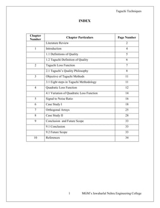
  • 1. Taguchi Techniques 1 MGM‟s Jawaharlal Nehru Engineering College INDEX Chapter Number Chapter Particulars Page Number Literature Review 2 1 Introduction 4 1.1 Definitions of Quality 5 1.2 Taguchi Definition of Quality 6 2 Taguchi Loss Function 7 2.1 Taguchi‟s Quality Philosophy 8 3 Objective of Taguchi Methods 11 3.1 Eight steps in Taguchi Methodology 11 4 Quadratic Loss Function 12 4.1 Variation of Quadratic Loss Function 14 5 Signal to Noise Ratio 16 6 Case Study I 18 7 Orthogonal Arrays 25 8 Case Study II 28 9 Conclusion and Future Scope 33 9.1 Conclusion 33 9.2 Future Scope 33 10 References 34
  • 2. Taguchi Techniques 2 MGM‟s Jawaharlal Nehru Engineering College LITERATURE REVIEW Paper No. Book / Research Paper Title Author Year 1. Taguchi Techniques for Quality Engineering. Phillip J. Ross 2005 2. Design and Analysis of Experiments. Douglas C. Montgomery 2001 3. Application of Taguchi method in the optimization of End Milling parameters J. A. Ghani I. A. Choudhary H. H. Hassan 2003 4. Optimisation of Deep Drilling Process Parameters of AISI 321 Steek using Taguchi Method Arshad Noor Siddiqueee Zahid A. Khan Mukesh Kumar 2014 5. Robust Design K. Sudhakar P. M. Mujumdar 2002 6. The Taguchi Methods of quality control examined: with reference to Sundstrand-Sauer Cheryl Lynn Moller-Wong 1988
  • 3. Taguchi Techniques 3 MGM‟s Jawaharlal Nehru Engineering College TABLE & GRAPH INDEX Table/ Graph Number Title of Table/ Graph Page Number G1 Traditional Quality Definition 6 G2 Taguchi Quality Definition 6 G3 Traditional Interpretation of Specification 8 G4 Time Temperature Relationship 10 G5 Nominal the better 14 G6 Smaller the better 14 G7 Larger the better 15 G8 Asymmetric 15 T1 Comparison between Signal to Noise Ratios 17 G9 Outer Diameter Histogram 18 G10 Outer Diameter Loss Function 19 T2 Cost of part versus outer Diameter 20 G11 Distribution due to tool wear 22 G12 Cost comparison 23 T3 Orthogonal Array 26 T4 Orthogonal Arrays 27 T5 23 Factorial Design 27 T6 24 Factorial Design 27 T7 Interaction Columns of an Orthogonal Array 29
  • 4. Taguchi Techniques 4 MGM‟s Jawaharlal Nehru Engineering College 1. INTRODUCTION When Japan began its reconstruction efforts after World War II, Japan faced an acute shortage of good quality raw material, high quality manufacturing equipment and skilled engineers. The challenge was to produce high quality products and continue to improve quality product under these circumstances. The task of developing a methodology to meet the challenge was assigned to Dr. Genichi Taguchi, who at that time was manager in charge of developing certain telecommunication products at the electrical communication laboratories (ECL) of Nippon Telecom and Telegraph Company (NTT). Through his research in the early 1960‟s, Dr Taguchi developed the foundation of Orthogonal Arrays and Robust design and validated his basics philosophies by applying them in the development of many products. He developed the concept of the Quality Loss Function in the 1970‟s. He also published the third and most current edition of his book on experimental designs. Genichi Taguchi made many important contributions during his lifetime in the field of quality control. The term Taguchi Methods is coined after him. Dr Taguchi received the individual DEMING AWARD in 1962, which is one of the highest recognition in the quality field. When the need is to have a process so robust that the process may not stay always within the specification but needs to stay centred at the target, Taguchi‟s Techniques are very useful. The underlying belief in this process is that every time a process moves away from the target there is loss to customer even if the process is within the specifications. This method focuses not only on the controllable factors as in conventional design of experiments but also considering the noise factors.
  • 5. Taguchi Techniques 5 MGM‟s Jawaharlal Nehru Engineering College 1.1 TRADITIONAL DEFINITION OF QUALITY The term, „Quality‟ was defined in the following way:  “Fitness for use”  Dr. Juran (1964)  The leading promoter of the “zero defects” concept and author of Quality is Free (1979) defines quality as” Conformance to requirements.  Philips Crosby  Quality should be aimed at needs of consumer, present and future.  Dr. Deming  The totality of features and characteristics of a product or service that bears on its ability to satisfy given needs.  The American Society for Quality Control (1983)  The aggregate of properties of a product determining its ability to satisfy the needs it was built to satisfy.  (Russian Encyclopedia)  The totality of features and characteristics of a product and service that bear on its ability to satisfy a given need.  (European Organization for Quality Control Glossary 1981) Although these definitions are all different, some common threads run through them:  Quality is a measure of the extent to which customer requirements and expectations are satisfied.  Quality is not static, since customer expectation can change.  Quality involves developing product or service specifications and standards to meet customer needs (quality of design) and then manufacturing products or providing services which satisfy those specifications and standards (quality of conformance). It is important to note that the above quality definitions which are before 1950‟s does not refer to grade or features. For example Honda Car has more features and is generally considered to be a higher grade car than Maruti. But it does not mean that it is of better quality. A couple with two children may find that a Maruti does a much better job of meeting their requirements in terms of case of loading and unloading ,comfort when the entire family is in the car, gas mileage, maintenance, and of course ,basic cost of vehicle.
  • 6. Taguchi Techniques 6 MGM‟s Jawaharlal Nehru Engineering College 1.2 TAGUCHI DEFINITION OF QUALITY Traditional Definition: The more traditional "Goalpost" mentality of what is considered good quality says that a product is either good or it isn't, depending or whether or not it is within the specification range (between the lower and upper specification limits -- the goalposts). With this approach, the specification range is more important than the nominal (target) value. But, is the product as good as it can be, or should be, just because it is within specification. G1 Taguchi Definition: Taguchi says no to above definition. He define the „quality‟ as deviation from on- target performance. According to him, quality of a manufactured product is total loss generated by that product to society from the time it is shipped. Financial loss or Quality loss. G2
  • 7. Taguchi Techniques 7 MGM‟s Jawaharlal Nehru Engineering College 2. TAGUCHI LOSS FUNCTION Taguchi loss function recognizes the customer‟s desire to have products that are more consistent, part to part, and a producer‟s desire to make low cost products. Genichi Taguchi has an unusual definition for product quality: “Quality is the loss a product causes to society after being shipped, other than any losses caused by its intrinsic functions.” By “loss” Taguchi refers to the following two categories. • Loss caused by variability of function. • Loss caused by harmful side effects. An example of loss caused by variability of function would be an automobile that does not start in cold weather. The car‟s owner would suffer a loss if he or she had to pay some to start a car. The car owner‟s employer loses the services of the employee who is now late for work. An example of a loss caused by a harmful side effect would be frost (cold) suffered by the owner of the car which would not start. An unacceptable product which is scrapped or rework prior to shipment is viewed by Taguchi as a cost to the company but not a quality loss. Taguchi suggests defining the function as follows: Loss (y) = 𝑘 𝑦 − 𝑚 2 Where, k = A / 𝑑2 And A = the cost of corrective action necessary to change the process d = the value of the process m = the target value of the process characteristic y = the measurement of the unit in question k = the loss coefficient Loss (y) = the incremental loss
  • 8. Taguchi Techniques 8 MGM‟s Jawaharlal Nehru Engineering College G3: Traditional interpretation of specification. 2.1 TAGUCHI’S QUALITY PHILOSOPHY Genichi Taguchi‟s impact on the word quality scene has been far- reaching. His quality engineering system has been used successfully by many companies in Japan and elsewhere. He stresses the importance of designing quality into product into processes, rather than depending on the more traditional tools of on-line quality control. Taguchi‟s approach differs from that of other leading quality gurus in that he focuses more on the engineering aspects of quality rather than on management philosophy of statistics. Also, Dr. Taguchi uses experimental design primarily as a tool to make products more robust- to make them less sensitive to noise factors. That is, he views experimental design as a tool for reducing the effects of variation on product and process quality characteristics. Earlier applications of experimental design focused more on optimizing average product performance characteristics without considering effects on variations. Taguchi‟s quality philosophy seven basic elements:
  • 9. Taguchi Techniques 9 MGM‟s Jawaharlal Nehru Engineering College 1. An important dimension of the quality of a manufactured product is the total loss generated by product to society. At a time when the BOTTOM LINE appears to be the driving force for so many organizations, it seems strange to see “loss to society” as part of product quality. 2. In a competitive economy, continuous quality improvement and cost reduction are necessary for staying in business. This is hard lesson to learn. Masaaki Imai (1986) argues very persuasively that the principal difference between Japanese and American management is that American companies look to new technologies and innovation as the major route to improvement, while Japanese companies focus more on “Kaizen” means gradual improvement in everything they do. Taguchi stresses use of experimental designs in parameter design as a way of reducing quality costs. He identifies three types quality costs: R & D costs, manufacturing costs, and operating costs. All three costs can be reduced through use of suitable experimental designs. 3. A continues quality improvement program includes continuous reduction in the variation of product performance characteristics about their target values. Again Kaizen. But with the focus on product and process variability this does not fit the mould of quality being of conformance to specification. 4. The customer‟s loss due to a product‟s performance variation is often approximately proportional to the square of the deviation of the performance characteristic from its target value. This concept of a quadratic loss function, says that any deviation from target results in some loss of the customer, but that large deviations from target result in severe losses. 5. The final quality and cost of manufactured product are determined to a large extent by the engineering designs of the product and its manufacturing process. This is so simple, and so true. The future belongs to companies, which, once they understand the variability‟s of their manufacturing processes using statistical process control, move their quality improvement efforts upstream to product and process design.
  • 10. Taguchi Techniques 10 MGM‟s Jawaharlal Nehru Engineering College 6. A product (or process) performance variation can be reduced by exploiting the nonlinear effects of the product (or process) parameters on the performance characteristics. This is an important statement because its gets to the heart of off-line QC. Instead of trying to tighten speciation beyond a process capability, perhaps a change in design can allow specifications to be loosened. As an example, suppose that in a heating process the tolerance on temperature is a function of the heating time in the oven. The tolerance relationship is represents by the band in given figure. For example : If a process specification says the heating process is to last 4.5 minutes, then the temperature must be held between 354.0 degrees and 355.0 degrees, a tolerance interval 1.0 degrees wide. Perhaps the oven cannot hold this tight a tolerance. One solution would be spending a lot of money on a new oven and new controls. Other possibility would be to change the time for the heating process to, say, 3.5 minutes. Then the temperature would need to be held to between 358.0 and 360.6 degrees an interval of width 2.6 degrees. If the oven could hold this tolerance, the most economical decision might be to adjust the specifications. This would make the process less sensitive to variation in oven temperature. G4: Time Temperature relationship 7. Statistically designed experiments can be used to identify the settings of product parameters that reduce performance variations. And hence improve quality, productivity, performance, reliability, and profits, statistically designed experiments will be the strategic quality weapon of the 1990‟s.
  • 11. Taguchi Techniques 11 MGM‟s Jawaharlal Nehru Engineering College 3. OBJECTIVE OF TAGUCHI METHODS The objective of Taguchi‟s efforts is process and product-design improvement through the identifications of easily controllable factors and their settings, which minimize the variation in product response while keeping the mean response on target. By setting those factors at their optimal levels, the product can be made robust to changes in operating and environmental conditions. Thus, more stable and higher-quality products can be obtained, and this is achieved during Taguchi‟ parameter-design stage by removing the bad effect of the cause rather than the cause of the bad effect. Furthermore, since the method is applied in a systematic way at a pre-production stage (off-line), it can greatly reduce the number of time-consuming tests needed to determine cost-effective process conditions, thus saving in costs and wasted products. 3.1 EIGHT-STEPS IN TAGUCHI METHODOLOGY 1. Identify the main function, side effects and failure mode. 2. Identify the noise factor, testing condition and quality characteristics. 3. Identify the objective function to be optimized. 4. Identify the control factor and their levels. 5. Select the Orthogonal Array, Matrix experiments. 6. Conduct the Matrix equipment. 7. Analyze the data; predict the optimum levels and performance. 8. Perform the verification experiment and plan the failure action.
  • 12. Taguchi Techniques 12 MGM‟s Jawaharlal Nehru Engineering College 4. QUADRATIC LOSS FUNCTION When an objective characteristic y deviates from its target value m, some financial loss will occur. Therefore, the financial loss, sometimes referred to simply as quality loss or used as an expression of quality level, can be assumed to be a function of y, which we shall designate L(y), When y meets the target m, the of L(y) will be at minimum; generally, the financial loss can be assumed to be zero under this ideal condition: L (m) = 0 ……………… Equation 2.1 Since the financial loss is at a minimum at the point, the first derivative of the loss function with respect to y at this point should also be zero. Therefore, one obtains the following equation: L΄ (m) = 0 …………….. Equation 2.2 If one expand the loss function L(y) through a Taylor series expansion around the target value m and takes Equations (2.1) and (2.2) into consideration, one will get the following equation: L(y) = L(m) + L΄ (m)(y-m)/1!+L΄΄(m)(y-m) ²/2!+ …………… =L΄΄(y-m)²/2! +……… Result is obtained because the constant term L(m) and the first derivative term L‟(m) are both zero. In addition, the third order and higher order term are assumed to be negligible. Thus, one can express the loss function as a squared term multiplied by constant k: L(y) =k(y-m)² …………… Equation 2.3
  • 13. Taguchi Techniques 13 MGM‟s Jawaharlal Nehru Engineering College When the deviation of the object characteristic from the target value increases, the corresponding quality loss will also increase. When magnitude of deviation is outside of the tolerance specifications, this product should be considered defective. Let the cost due to defective product be A and the corresponding magnitude of the deviation from the target value be. Taking into right hand side of Equation (2.3), one can determine the value for constant k by following Equation: k=cost of defective product / (tolerance)² Consider the visitor to the BHEL Heavy Electric Equipment Company in India who was told, “In our company, only one unit of product needs to be made for our nuclear power plant. In fact, it is not really necessary for us to make another unit of product. Since the sample size is only one, the variance is zero. Consequently, the quality loss is zero and it is not really necessary for us to apply statistical approaches to reduce the variance of our product.” However, the quality loss function [L = k(y – m) ²] is defined as the mean square deviation of objective characteristics from their target value, not the variance of products. Therefore, even when only one product is made, the corresponding quality loss can still be calculated by Equation (2.3). Generally, the mean square deviation of objective characteristics from their target values can be applied to estimate the mean value of quality loss in Equation (2.3). One can calculate the mean square deviation from target σ² (σ² in this equation is not variance) by the following equation (the term σ² is also called the mean square error or the variance of products):
  • 14. Taguchi Techniques 14 MGM‟s Jawaharlal Nehru Engineering College 4.1 VARIATION OF THE QUADRATIC LOSS FUNCTION Nominal the best type: Whenever the quality characteristic y has a finite target value, usually nonzero, and the quality loss is symmetric on the either side of the target, such quality characteristic called nominal-the-best type. This is given by equation L(y) =k(y-m) ² G5 Colour density of a television set and the output voltage of a power supply circuit are examples of the nominal-the-best type quality characteristic. Smaller-the-better type: Some characteristic, such as radiation leakage from a microwave oven, can never take negative values. Also, their ideal value is equal to zero, and as their value increases, the performance becomes progressively worse. Such characteristic are called smaller-the- better type quality characteristics. The response time of a computer, leakage current in electronic circuits, and pollution from an automobile are additional examples of this type of characteristic. The quality loss in such situation can be approximated by the following function, which is obtain from equation by substituting m = 0 L(y) =ky² This is one side loss function because y cannot take negative values. G6
  • 15. Taguchi Techniques 15 MGM‟s Jawaharlal Nehru Engineering College Larger-the-better type: Some characteristics, such as the bond strength of adhesives, also do not take negative values. But, zero is there worst value, and as their value becomes larger, the performance becomes progressively better-that is, the quality loss becomes progressively smaller. Their ideal value is infinity and at that point the loss is zero. Such characteristics are called larger-the-better type characteristics. It is clear that the reciprocal of such a characteristics has the same qualitative behaviour as a smaller-the-better type characteristic. Thus we approximate the loss function for a larger-the-better type characteristic by substituting 1/y for y in L(y) = k [1/y²] G7 Asymmetric loss function: In certain situations, deviation of the quality characteristic in one direction is much more harmful than in the other direction. In such cases, one can use a different coefficient k for the two directions. Thus, the quality loss would be approximated by the following asymmetric loss function: k ( y – m ) ²,y > m L(y) = k(y-m) ², y ≤ m G8
  • 16. Taguchi Techniques 16 MGM‟s Jawaharlal Nehru Engineering College 5. SIGNAL TO NOISE RATIO In Taguchi designs, a measure of robustness used to identify control factors that reduce variability in a product or process by minimizing the effects of uncontrollable factors (noise factors). Control factors are those design and process parameters that can be controlled. Noise factors cannot be controlled during production or product use, but can be controlled during experimentation. In a Taguchi designed experiment, you manipulate noise factors to force variability to occur and from the results, identify optimal control factor settings that make the process or product robust, or resistant to variation from the noise factors. Higher values of the signal-to-noise ratio (S/N) identify control factor settings that minimize the effects of the noise factors. Taguchi experiments often use a 2-step optimization process. In step 1 use the signal-to- noise ratio to identify those control factors that reduce variability. In step 2, identify control factors that move the mean to target and have a small or no effect on the signal-to- noise ratio. The signal-to-noise ratio measures how the response varies relative to the nominal or target value under different noise conditions. You can choose from different signal-to- noise ratios, depending on the goal of your experiment. For static designs, Minitab offers four signal-to-noise ratios as shown in figure. The Nominal is Best (default) signal-to-noise ratio is useful for analyzing or identifying scaling factors, which are factors in which the mean and standard deviation vary proportionally. Scaling factors can be used to adjust the mean on target without affecting signal-to-noise ratios.
  • 17. Taguchi Techniques 17 MGM‟s Jawaharlal Nehru Engineering College T1: Comparison between Signal to Noise Ratios
  • 18. Taguchi Techniques 18 MGM‟s Jawaharlal Nehru Engineering College 6. CASE STUDY I Tool Wear in a Process This case study is intended to show cost-oriented approach to quality control. With a very capable process goalpost philosophy allows tool wear to produce parts which vary from one specification limit to other. The lost function economically justifies different quality control approach. An important aspect of product and process quality is the relative width of the distribution and the specification limits of the product. If the distribution is narrower than the specification limits of the products, then it is possible to make all or nearly all parts. All of this is desirable from goalpost point of view. A typical tolerance of machined part is to be +- 0.25mm. A process that would be very capable with respect to this tolerance would be modelled as shown in figure. G9: Outer Diameter Histogram. The Taguchi loss function quantifies the variability present in a process. If a part reaches the end of the manufacturing line with diameter exceeding the upper or lower limit, the part should be scrapped at $4.00. The scrap cost is one aspect of loss to society. Using the cost as a reference value, a loss function can be constructed as shown in figure. Taguchi uses the mathematical equation to model this picture of cost v/s outer diameter. Loss (y) = 𝑘 𝑦 − 𝑚 2
  • 19. Taguchi Techniques 19 MGM‟s Jawaharlal Nehru Engineering College G10: Outer Diameter Loss Function. This equation, L is the loss associated with a diameter value y, m is the nominal value of specification, and value of k is a constant depending upon the cost at the specification limits and the width of specification. L = 𝑘 𝑦 − 𝑚 2 $4.00 = k 𝐿𝑆𝐿 – 𝑚 2 The lower specification limit (LSL) is substituted into equation, which is where the $4.00 loss is incurred. The upper specification limit also could be used for this calculation. Solving for k, 𝑘 = $4.00 𝐿𝑆𝐿 – 𝑚 2 𝑘 = $4.00 −0.010 – 0.0 2 k = $40,000 per sq in. L = 40,000 𝑦 − 0.0 2 Now the loss associated with any part can be computed depending on the value of its diameter.
  • 20. Taguchi Techniques 20 MGM‟s Jawaharlal Nehru Engineering College For instance, a part with diameter of + 0.003 in (+ 0.08 mm) costs L = 40,000 0.003 − 0.0 2 L = $ 0.36 This is the loss per unit for each part shipped with an outer diameter of +0.003 in. Similarly for a part diameter of -0.002 in which are 11 quantities in number the cost incurred would be, L ( - 0.002 ) = $ 40,000 −0.002 − 0.0 2 = $ 0.16 x 11 = $1.76 𝐿 = $10.56 100 𝑃𝑎𝑟𝑡𝑠 $0.11 per part T2: Cost of part versus outer Diameter
  • 21. Taguchi Techniques 21 MGM‟s Jawaharlal Nehru Engineering College A second method of estimating average loss per part entails using the loss equation in a slightly modified form. Mathematically, this calculation is equivalent to using the average value of the 𝑦 − 𝑚 2 portion of the loss equation. 𝐿 = 𝑘[ 𝑦1 − 𝑚 2 + 𝑦2 − 𝑚 2 + … + 𝑦𝑛 − 𝑚 2 ] 𝑁 Where, N: number of parts sampled If all the values of (y – m) values are squared, added together and divided by the number of items, then the result is desired value. For a large number of parts, the average loss per part is equivalent to 𝐿 = 𝑘 𝑆2 + 𝑦 − 𝑚 2 𝑆2 : Variance around the average. 𝑦 : Average value of y for the group. 𝑦 − 𝑚 : Offset of the group average. 𝑆2 = 2.64 x 10⁻⁶ 𝑖𝑛2 𝑦 = 0.0 𝐿 = 𝑘 𝑆2 + 𝑦 − 𝑚 2 𝐿 = 40,000 2.64 𝑋 10−6 + 0.0 − 0.0 2 𝐿1 = $ 0.11 per part This second method uses the general loss function for a nominal is best situation.
  • 22. Taguchi Techniques 22 MGM‟s Jawaharlal Nehru Engineering College This example demonstrates the loss associated with a distribution that has a very good process capability ratio and is centrally located on the target value of 0.0 in. Traditional quality control would cause a situation where there would be a variation in size. The loss function uses the average and variance for a group of parts to calculate loss. For a group of parts where the distribution average is continually increasing, the variance is G11: Distribution due to tool wear 𝑆 𝑅𝑒𝑠𝑢𝑙𝑡𝑎𝑛𝑡 2 = 𝑆 𝑂𝑟𝑖𝑔𝑖𝑛𝑎𝑙 2 + 𝑊2 12 Where W is the width of tool wear allowed. 𝑆 𝑂 2 = 2.64 𝑥 10−6 𝑖𝑛2 W = 0.010 in 𝑆 𝑅 2 = 2.64 𝑥 10−6 + 0.0102 12 = 1.10 x 10⁻⁵
  • 23. Taguchi Techniques 23 MGM‟s Jawaharlal Nehru Engineering College The loss per part is then, 𝐿 = 𝑘 𝑆2 + 𝑦 − 𝑚 2 𝐿2 = $ 40,000 1.10 𝑥 10−5 + 0 − 0 2 = $ 0.44 It is clear that, Loss of centred distribution is less than that of a distribution which traverses the specification range. L1 < L2 But to obtain a low loss the machine would have to be adjusted after each part. For the second situation, the machine would not have to be adjusted nearly as often. Therefore, there must be compromise between loss function and adjustment costs. Ca = adjustment cost per part for N parts La = k 𝑊2 12 N = number of parts made since last adjustment N = W / R R = wear rate of tool G12: Cost comparison
  • 24. Taguchi Techniques 24 MGM‟s Jawaharlal Nehru Engineering College Ca = R x (total m/c adjustment cost / W) The true optimisation cost is at 0.005 in tool wear span, but the additional loss of going up to 0.006 in total span is very minimal ($ 0.003), which is beyond the accuracy of the loss function. Adjustment width is 0.006 in, i.e. + 0.003 to –0.003 to get a centred nominal value of 0.0 in as the optimum adjustment interval depends upon the scrap loss of a part. This case study shows the economic penalty of allowing excessive variation in a product or a process. Taguchi uses a very comprehensive economic approach to on-line production quality control.
  • 25. Taguchi Techniques 25 MGM‟s Jawaharlal Nehru Engineering College 7. ORTHOGONAL ARRAYS An Array‟s name indicates the number of rows and column it has, and also the number of levels in each of the column. Thus the array L4 (2³) has four rows and three 2-level column. Historically, related methods was developed for agriculture, largely in UK, around the Second World War, Sir R.A.Fisher was particularly associated with this work. Here the field area has been divided up into rows and column and four fertilizers (F1-F4) and four irrigation levels are represented. Since all combination are Taken, sixteen „cells‟ or „plots‟ result. The Fisher field experiment is a full factional experiment since all 4*4 =16 combinations of the experiments factors, fertilizer and irrigation level, are included. The number of combinations required may not be feasible or economic. To cut down on the number of experimental combinations included, a Latin Square design of experiment may be used. Here there are three fertilisers, three irrigation levels and three alternative additives (A1-A2) but only nine instead of the 3*3*3 =27 combination, of the full factorial are included. There are „pivotal‟ combinations, however, that still allow the identification of the best fertiliser, Irrigation level and additive provided that these no serious non-additives or interactions in the relationship between yield and these control factors. The property of Latin Squares that corresponds to this is that each of the labels A1, A2, A3 appears exactly once in each row and column.
  • 26. Taguchi Techniques 26 MGM‟s Jawaharlal Nehru Engineering College Difference from agricultural applications is that in agriculture the „noise‟ or uncontrollable factors that disturb production also tend to disturb experimentation, such as the weather. In industry, factors that disturb production, or are uneconomic to control in production, can and should be directly manipulated in test. Our desire is to identify a design or line calibration which can best survive the transient effects in the manufacturing process caused by the uncontrolled factors. We wish to have small piece to piece and time to time variations associated with this noise variation. To do this we can force diversity on noise conditions by crossing our orthogonal array of controllable factors by full factorial or orthogonal array of noise factors. Thus in the example, we evaluate our product for each of the nine trials against the background of four different combinations of noise conditions. We are looking one of the nine rows of control factors combinations, or for one of the „missing‟ 72 rows ({3*3*3*3}=81; 81-9=72), which not only gives the correct mean result on average, but also minimises variation away from the mean. T3: Orthogonal Array Orthogonality is represented as ∑xi. xj = 0 for all the pairs of levels, where i, j represent high and low (+1, -1) levels. Advantage of orthogonality is that each factor can be evaluated independently.
  • 27. Taguchi Techniques 27 MGM‟s Jawaharlal Nehru Engineering College ORTHOGONAL ARRAYS T4: Orthogonal Arrays T5: 23 Factorial Design T6: 24 Factorial Design
  • 28. Taguchi Techniques 28 MGM‟s Jawaharlal Nehru Engineering College 8. CASE STUDY II Consider a process, of producing steel springs, is generating considerable scrap due to cracking after heat treatment. A study is planned to determine better operating conditions to reduce the cracking problem. There are several ways to measure cracking - Size of the crack - Presence or absence of cracks The response selected was Y: the percentage without cracks in a batch of 100 springs Three major factors were believed to affect the response - T: Steel temperature before quenching - C: carbon content (percent) - O: Oil quenching temperature Experiment: Four runs at each level of T with C and O at their low levels Problem: How general is this conclusion? Does it depend upon? - Quench Temperature? - Carbon Content? - Steel chemistry? - Spring type?
  • 29. Taguchi Techniques 29 MGM‟s Jawaharlal Nehru Engineering College Factorial Approach: - Include all factors in a balanced design: - To increase the generality of the conclusions, use a design that involves all eight combinations of the three factors. The treatments for the eight runs are given as under: T7: Interaction Columns of an Orthogonal Array. The above eight runs constitute a FULL FACTORIAL DESIGN. The design is balanced for every factor. This means 4 runs have T at 1450 and 4 have T at 1600. Same is true for C and O. IMMEDIATE ADVANTAGES - The effect of each factor can be assessed by comparing the responses from the appropriate sets of four runs. - More general conclusions - 8 run rather than 24 runs. The data for the complete factorial experiment are: The main effects of each factor can be estimated by the difference between the average of the responses at the high level and the average of the responses at the low level. For example to calculate the O main effect:
  • 30. Taguchi Techniques 30 MGM‟s Jawaharlal Nehru Engineering College Avg. of responses with O as 70 = (67 + 61+ 79 + 75) / 4 = 70.5 Avg. of responses with O as 120 = (59 + 52 + 90 + 87) / 4 = 72 So the main effect of O is = 72.0 - 70.5 = 1.5 The apparent conclusion is that changing the oil temperature from 70 to 120 has little effect. The use of factorial approach allows examination of two factor interactions. For example we can estimate the effect of factor O at each level of T. At T = 1450 Avg. of responses with O as 70 = 64.0 = (67 + 61) / 2 Avg. of responses with O as 120 = 55.5 = (59 + 52) / 2 So the effect of O is 55.5 – 64 = -8.5 At T = 1600 Avg. of responses with O as 70 = 77.0 = (79 + 75) / 2 Avg. of responses with O as 120 = 88.5 = (90 + 87) / 2 So the effect of O is 88.5 – 77 = 11.5 The conclusion is that at T = 1450, increasing O decreases the average response by 8.5 whereas at T = 1600, increasing O increases the average response by 11.5. That is, O has a strong effect but the nature of the effect depends on the value of T. This is called interaction between T and O in their effect on the response. It is convenient to summarize the four averages corresponding to the four combinations of T and O in a table:
  • 31. Taguchi Techniques 31 MGM‟s Jawaharlal Nehru Engineering College When an interaction is present the lines on the plot will not be parallel. When an interaction is present the effect of the two factors must be considered simultaneously. The lines are added to the plot only to help with the interpretation. We cannot know that the response will increase linearly. Two way tables of averages and plots for the other factor pairs are:
  • 32. Taguchi Techniques 32 MGM‟s Jawaharlal Nehru Engineering College Result: - C has little effect - There is an interaction between T and O. Recommendations: - Run the process with T and O at their high levels to produce about 90% crack free product (further investigation at other levels might produce more improvement). - Choose the level of C so that the lowest cost is realized.
  • 33. Taguchi Techniques 33 MGM‟s Jawaharlal Nehru Engineering College 9. 9.1 CONCLUSION Taguchi method is a very popular offline quality method. Many Taguchi practitioners have used engineering knowledge to resolve multi-response optimization problems. However, it cannot solve the multi-response problem which occurs often in today‟s environment. Research shows that the multi-response problem is still an issue with the Taguchi method. In this work, two different approaches to overcome these problems are presented. The proposed approaches use weight-based desirability method and weight based grey relation analysis to optimize the parameter design. Three existing industrial cases from literature demonstrate the effectiveness of the proposed approaches. The proposed approaches posses the following merits.  They are applicable for solving both quantitative and qualitative parameters.  They are simple and easy to apply in real cases in manufacturing, especially when dealing with multiple responses.  Researchers with limited knowledge in mathematical background can also apply these approaches. The Taguchi approach to quality engineering places a great deal of emphasis on minimizing variation as the main means of improving quality. The idea is to design products and processes whose performance is not affected by outside conditions and to build this in during the development and design stage through the use of experimental design. The method includes a set of tables that enable main variables and interactions to be investigated in a minimum number of trials. 9.2 SCOPE FOR FURTHER RESEARCH Apart from these Desirability Method and Grey Relation Analysis, new methods can also be developed for solving the multi-response problems with censored data in the Taguchi method. A weighted principle component analysis and evolutionary optimization techniques can also be developed to select the optimal parameters to yield the best results. Also hybrid algorithms and techniques may be developed depending upon the applications.
  • 34. Taguchi Techniques 34 MGM‟s Jawaharlal Nehru Engineering College 10. REFERENCES 1. Phillip J. Ross, “Taguchi Techniques for Quality Engineering”, Tata McGraw-Hill Publishing Company, 2005. 2. Douglas C. Montgomery, “Design and Analysis of Experiments”, Wiley Publications, 2001. 3. Park, Sung H, “Robust Design and Analysis for Quality Engineering”, Chapman & Hall, London, 1996. 4. Bagchi, Tapan P, “Taguchi Methods Explained: Practical Steps to Robust Design”, Prentice Hall of India, New Delhi, 1993. 5. Madhav. S. Phadke, “Quality Engineering Using Robust Design”, Prentice Hall / AT&T, New jersey, USA, 1989. 6. Patrick N. Koch, Timothy W. Simpson, Janet K. Allen, and Farrokh Mistree, “Statistical Approximation for Multidisciplinary Design optimization: The Problem of Size”, Journal of Aircraft : Special Issue on Multidisciplinary Design Optimization, vol.36, 1999, pp 275-286. 7. Wei Chen, Kemper Lewis, “A Robust Design Approach for Achieving Flexibility in Multidisciplinary Design”, http:/www.uic.edu/labs/ideal/pdf/Chen-Lewis.pdf Luc Huyse, “Solving Problems of Optimization Under Uncertainty as Statistical Decision Problems”, AIAA-2001-1519, 2001. 8. Wei Chen, Xiaoping Du, “Efficient Robustness and Reliability Assessment in Engineering Design”, www.icase.edu/colloq/data/colloq.Chen.Wei2001.5.9.html 9. Robert H. Sues, Mark A.Cesare, Stephan S. Pageau, & Justin Y.-T.Wu,
  • 35. Taguchi Techniques 35 MGM‟s Jawaharlal Nehru Engineering College “Reliability – Based Optimization Considering Manufacturing and Operational Uncertainties”, Journal of Aerospace Engineering, October, 2001, pp 166-174 10. Brent A. Cullimore , “Reliability Engineering & Robust Design : New Methods for Thermal / Fluid Engineering”, C & R White Paper, Revision 2, May 15, 2000 http://www.sindaworks.com/docs/papers/releng1.pdf 11. Luc Huyse, R. Michael Lewis, “Aerodynamic Shape Optimization of Twodimensional Airfoil Under Uncertain Conditions”, NASA/CR-2001-210648 12. Timothy W. Simpson, Jesse Peplinski, Patric N. Koch, and Janet K. Allen, “On the Use of Statistics in Design & the Implications for Deterministic Computer Experiments”, ASME Design Engineering Technical Conference, California, 1997. 13. Luc Huyse, “Probabilistic Approach to Free-Form Airfoil Shape Optimization Under Uncertainty”, AIAA Journal, Vol. 40, No.9, September, 2002 14. K.K.Choi, B.D.Youn, “Issues Regarding Design Optimization Under Uncertainty”, http://design1.mae.ufl.edu/~nkim/index-files/choi4.pdf 15. A.K. Kundu, John Watterson, and S. Raghunathan, “Parametric Optimization of Manufacturing Tolerances at the Aircraft Surface” Journal of Aircraft, Vol.39, No.2, March-April 2002.