SlideShare a Scribd company logo
1 of 29
BUS 308 Week 2 Lecture 2
Statistical Testing for Differences – Part 1
After reading this lecture, the student should know:
1. How statistical distributions are used in hypothesis testing.
2. How to interpret the F test (both options) produced by Excel
3. How to interpret the T-test produced by Excel
Overview
Lecture 1 introduced the logic of statistical testing using the
hypothesis testing procedure.
It also mentioned that we will be looking at two different tests
this week. The t-test is used to
determine if means differ, from either a standard or claim or
from another group. The F-test is
used to examine variance differences between groups.
This lecture starts by looking at statistical distributions – they
underline the entire
statistical testing approach. They are kind of like the
detective’s base belief that crimes are
committed for only a couple of reasons – money, vengeance, or
love. The statistical distribution
that underlies each test assumes that statistical measures (such
as the F value when comparing
variances and the t value when looking at means) follow a
particular pattern, and this can be used
to make decisions.
While the underlying distributions differ for the different tests
we will be looking at
throughout the course, they all have some basic similarities that
allow us to examine the t
distribution and extrapolate from it to interpreting results based
on other distributions.
Distributions. The basic logic for all statistical tests: If the null
hypothesis claim is
correct, then the distribution of the statistical outcome will be
distributed around a central value,
and larger and smaller values will be increasingly rare. At some
point (and we define this as our
alpha value), we can say that the likelihood of getting a
difference this large is extremely
unlikely and we will say that our results do not seem to come
from a population that matches the
claims of the null hypothesis.
Note that this logic has several key elements:
1. The test is based on an assumption that the null hypothesis is
correct. This gives us a
starting point, even if later proven wrong.
2. All sample results are turned into a statistic that matches the
test selected (for
example, the F statistic when using the F-test, or the t-statistic
when using the T-test.)
3. The calculated statistic is compared to a related statistical
distribution to see how
likely an outcome we have.
4. The larger the test statistic, the more unlikely it is that the
result matches or comes
from the population described by the null hypothesis claim.
We will demonstrate these ideas by looking at the questions
being asked in this week’s
homework. We will show results of the related Excel tests, and
discuss how to interpret the
output.
We need to remember that seeing different value (mean,
variance, etc.) from different
samples does not tell us that the population parameters we are
estimating are, in fact, different.
The one thing we know about sampling is that each sample will
be a bit different. They
generally provide a “close enough” estimate to the population
values of concern for decision and
action purposes. But, they are not an exact match. This
difference is examined by the use of the
statistical tests, which tell us how much importance we should
attach to observed differences.
Lecture Examples
The lectures for each week will also look at our class question
of whether or not males
and females are paid equally for equal work. These additional
analyses provide some different
clues on what the data is trying to tell us about company pay
practices.
While your analysis will focus directly on the salary that males
and females are being
paid, the lecture examples will use an alternate method of
examining pay practices. Many
compensation professionals often use a relative pay measure
called the “comparison-ratio,” or
compa-ratio, to examine pay patterns within the company.
Some background on this measure. Many companies use grades
to group jobs of equal
value to the company into groups that have a similar pay range
– the values that a company is
willing to pay employees for the job. (As strong as a performer
a mail room clerk is, they will
rarely be paid the same as the CEO.) Many companies will set
the middle of this range, the
midpoint, as the average salary that that market pays to hire
someone into the job. This is how
companies remain competitive in their hiring.
Now, compensation professionals will generally want to analyze
how the company is
paying employees relative to these market rates (as summarized
by the midpoint). One approach
is to divide each employee’s salary by its related midpoint. The
outcome is the compa-ratio
which is considered an alternate measure of pay that eliminates
the impact of different grades.
The compa-ratio reports pay as a ratio of the actual salary
divided by the salary grade’s midpoint.
The compa-ratio shows if an employee is being paid more than
the midpoint (measure’s
value > 1.0) or less than the midpoint (< 1.0). This measure
allows us to look at salary
dispersion within a company without focusing on the exact
dollar values. It allows a comparison
between what the company is paying and what the outside
market is paying (which most
company’s target as the midpoint of a salary range) for the jobs.
The compa-ratio shows if employees are paid above or below
the grade midpoint and it
can be used to see what the dispersion pattern of pay. Equal
pay would expect to see similar
distributions, variances and means, between males and females
in this measure.
The lecture examples will cover the same statistical tests as the
homework assignments
but will focus on the compa-ratio pay measure rather than
salary. As such, the results presented
each week should be included and/or factored into your weekly
conclusions on what the data has
told us about the answer to our question.
The first step in looking at whether males and females are paid
equally would be to look
at the average pay of each. Given our sample is a random
sample of the population of employees
(and, therefore considered to be representative of the
population), the average salaries or average
compa-ratios (they measure related but not identical measures
of pay) will give us an indication
of whether things are the same for each gender or not.
One issue in looking at averages is the variation within the
groups. If both groups have
the same or very similar variation across the salaries then we
test the averages for a difference
using one approach. If the group variances are significantly
different, we use a slightly
approach. So, the first step is to examine group variances. This
is done with the F-test.
F-test
As noted, the F-test is used to compare variances to determine if
the differences noted
could be from simple sampling error (also known as pure chance
alone) or if the differences are
large enough to be considered statistically different. The F
statistic is simply one group’s
variance divided by the other group’s variance. (When done by
hand, it is traditional to have the
largest variance in the numerator, but this is not critical when
Excel performs the test for us.) So,
if the variances are equal, then the result of one variance
divided by the other would equal 1.0 –
this is the center of the F distribution. How about a situation
where one variance equaled 4 and
the other equaled 5 (randomly picked numbers for this
example)? If we divided the larger by the
smaller, we would get 5/4 = 1.25 while if we divided the
smaller by the larger, we would get 0.8.
Note that these values are on each side of the center value of
1.00. This is what is meant by “two
tails” with the F-test – one tail of the distribution has values
less than 1.0 while the other has
values greater than 1.0.. Our value of F depends first on the
variances (of course) and then on
how we do the division. The likelihood of these two variances
coming from populations that
have the same variance does not depend upon which tail the
result is in, but rather how likely it is
to see a difference from 1.00. This is given to us by the F-test
p-value (probability value of
seeing a difference as large or larger than what we have if the
null hypothesis is true).
One new concept introduced with the F-test is the idea of
degrees of freedom (df). While
the technical explanation is somewhat tedious, we can
understand the concept with a simple
example. If we have 5 numbers, for example: 1, 2, 3, 4, and 5;
we also have a sum of them; in
this case 15. Now, assume we can change any of the numbers in
the data set with the only
requirement being that the total must remain the same. How
many of the numbers are we free to
change; or what is our degree of freedom in making changes?
In this case, we can change any 4
of the values, as soon as we do so we automatically get the fifth
value (whatever is needed to
make the sum equal to 15). Thus, to generalize, our df is the
count we have minus 1 (equaling n
-1). N-1 is the formula for the degrees of freedom for each
variable in the F-test. We will se this
idea in other statistical tests, each of which has its own formula
to calculate it. The nice thing is
that Excel will give us this outcome without our needing to
worry about it, and we rarely have to
actually use it in any of our work – but, it is technically part of
most statistical tests.
There are two versions of the F-test available for use. One is
located in the Data ribbon
under the Analysis block in the Data Analysis link and is called
F-Test Two-Sample for
Variances. The other is located in the Fx Statistical list (which
is duplicated in the Formulas
ribbon under the More Functions option and the Statistical list)
and is called simply F.test.
While both test variances, there is an important difference. The
F-Test Two Sample for
Variances option provides some additional summary statistics
(mean, variance, count) for each
sample, but only provides a one-tail test outcome. One-tail
results, whether with the F-Test or
the T-test are used to test a directional difference in variances,
when we want to know if one
variance is larger (or smaller) than the other. Since, in general
we are interested in the simpler
question of whether the variances are equal or not (without
regard to which is larger), when
using this form to test for equality or not, we need to double the
p-value to find the two t-tail p-
value we need for our decision on rejecting the null hypothesis.
On the other hand, the F.test found in Fx or Formulas returns
only the two-tail p-value;
enough for a decision on rejecting or failing to reject the null
hypothesis of no difference but
nothing else. Technically, this is the version we should use
when conducting our two-tail
questions in the homework, but (as noted) either can be used if
we remember to double the p-
value for the one -tail outcome.
Example: Testing for Variance Equality
As mentioned above, it is often beneficial to start with looking
at variance equality when
comparing groups. We need to start our analysis of equal pay
for equal work by seeing if there is
even an issue to be concerned with. So, we have selected our
random sample of 25 males and 25
females from our corporate population. (A couple of
assumptions; the company exists in only
one location, and all our employees in the sample are exempt
professions or managers with at
least a bachelor’s college degree.)
Our initial question is: Are the male and female compa-ratio
variances equal? (Note, if
they are, this would mean that the standard deviations of both
groups are the same.) As with all
statistical tests, we will be using our samples to make
judgements or inferences about the
population values. While the sample result values will differ,
this difference may not be large
enough to show that the population values are not the same.
Question 1. One of the first things of interest to detectives is if
the behavior of the
suspects differs from what they normally do. That is, who’s
behavior varies from the norm?
Relating this to our compa-ratio measures has us asking if the
compa-ratio variance for males
and females are equal within the population. (In the homework,
the question asks about salary
variances. The logic and approach for answering the salary-
based question is the same as shown
below.)
Variance equality is tested using the F-Test. There are two
versions of this test available
to us that we could use, and both will be shown below. Note
that equal standard deviations do
not automatically mean that the means are close, it just tells us
if the dispersion patterns are
similar. If similar, the means of each group can be considered
equally reflective of the data. The
following focuses on just setting up the data for and performing
the statistical test.
The following show only the output for the six hypothesis
testing steps. How the Excel
F-tests are set up is covered in Lecture 3 for this week.
Step 1: The question asked is whether the variances for males
and females are equal. The
hypothesis statements for an equality test are shown below.
Ho: Male compa-ratio variance = Female compa-ratio variance
Ha: Male compa-ratio variance =/= Female compa-ratio
variance
(Since the question asks about equality and not a directional
difference, this is a two-tail
test. The Null must contain the names of the two variables
involved (Male and Female),
the statistic being tested (variance), and the relationship sign
(=). The alternate provides
the opposite view so that between them all possible outcomes
are covered. We are only
concerned if the variances are equal, not whether one or the
other is larger (or smaller).)
Step 2: We state our decision-making criteria here. It is: Alpha
= 0.05 (This will be the
same for all statistical tests we perform in the class, and
therefore the same in all
hypothesis set-ups.)
Step 3: The test, test statistic, and the reason for selecting the
test are stated here. For this
example, we are using: F statistic and F-test for Variance. We
use these as they are
designed to test variance equality.
Step 4: Our decision-making rule is presented here: Reject the
null hypothesis if the p-
value is < alpha = 0.05.
(This step is also the same for every statistical test we will
perform; it says we will reject
the null hypothesis if the probability of getting a result as large
as what we see is less than
5% or a probability of 0.05.)
Note that these steps are set-up before we even look at the data.
While, we may have set
up the data columns, we should not have done any analysis yet.
These steps tell us how
we will make a decision from the results we get.
Step 5: Perform the analysis. This is the step where Excel
performs the analysis and
produces output tables. The setting up of each Excel test is
covered in Lecture 3, we are
primarily interested in how to interpret the results in this
lecture.
Here is a screenshot of the results for both versions of the F-
test. (Only one is needed for
the question.)
Step 6: Conclusions and Interpretation. This is where we
interpret what the data is trying
to tell us.
Before moving on to interpreting these results, let’s look at
what we have. The F-Test
Two-Sample for Variances output clearly has more information
than the F.TEST. We
have the labels identifying each group as well as the mean,
variance, and count
(Observations) for each group. The df, equaling the (sample
size -1), is shown as well as
the calculated F statistic (which equals the left group’s (or Male
in this case) variance
divided by the right group’s (Female) variance. Note, Excel
divides the variances in the
order that they were entered into the data entry box, for this
example the Males were
entered first.
The next two rows are critical for our decision making; but they
are incomplete. They
show the one-tail critical values used in decision making. The
P(F<=f) one-tail is the P-
value, or the probability of getting an F-value as large or larger
than we have if the null
hypothesis is true. However, it is only a one-tail outcome,
while we want a two-tail
outcome, since we only care about the variances being equal or
not, not which one is
larger. So, the result as presented cannot be used directly.
What we need to do will be
covered after we look at the F.TEST result.
The F.TEST gives less information, but it provides us with
exactly what we need; the
two-tail p-value. For our data set, we have a 40% (rounded)
chance of getting an F value
this large or larger purely by chance alone when we are looking
at a two-tail outcome.
Note that this value, 0.39766 is twice the one-tail value of
0.19883 from the F-Test table.
This will always be true, the two-tail probabilities will be twice
the one-tail values.
So, if we want to use the F-TEST Two-Sample for Variance
tool, we need to double the
p-value before making our step 6 decisions.
We are now ready to move on to what step 6 asks for. This step
has several parts.
• What is the p-value: 0.3977 (our compa-ratio example result).
This value equals
EITHER tht F.TEST outcome or 2 times the F-test result. (If,
the F-test p-value is
in cell K-15, you could enter =2*K15 to get the value desired).
• What is your decision: REJ or Not reject the null? (If our p-
value is < (less than)
0.05, we say REJ, if the p-value is > (larger than) 0.05, we say
NOT reject. This is
what our decision rule says to do.) Our answer is for compa-
ratio variances:
NOT Rej. This means we do not reject the claim made by the
null hypothesis
and accept it as the most likely description of the variances
within the population.
• Why? This line asks us to explain why we made the decision
we did. Our compa-
ratio response is: The p-value is > (greater than) 0.05, and the
decision rule is
reject if the p-value was < 0.05. (The answer here is simply
why, based on the
reasoning shown above, you chose your REJ or NOT Rej
choice.)
• What is your conclusion about the variances in the population
for the male and
female salaries? This part asks us to translate the statistical
decision into a clear
answer to the initial question (Are male and female compa-
values equal?) Our
response: We do not have enough evidence to say that the
variances differ in
the population. The variances are equal in the population. Had
we rejected
the null hypothesis, we would have said the population
variances differed.
Note that this question did not tell us anything about actual pay
differences between the
genders. It did tell us that both groups are dispersed in a
similar manner, and thus supported
some of the conclusions we drew from looking at the data last
week.
Examples: Testing for Mean Equality
While we test for variance equality with an F test, we use the T-
Test to test for mean
equality testing. The t-test also uses the degree of freedom (df)
value in providing us with our
probability result; but again, Excel does the work for us. The t
distribution is a bell-shaped curve
that is flatter and a bit more spread out than the normal curve
we discussed last week. The center
is located at 0 (zero) and the tails (the negative and positive
values) are symmetrical.
The t statistic for the testing of two means is basically: (Mean1
– Mean2)/standard error
estimate. (The standard error formula varies according to which
type of t-test we are
performing.) Note that the t will be either positive or negative
depending upon which mean is
larger. So, if we are interested in simply equal or not equal, it
does not matter if we have a
positive or negative t value, only the size of the difference
matters. As with the F-test, half of
our alpha goes in the positive tail and half goes in the negative
tail when making our equality
decision.
We have two questions about means this week.
Question 2. The second question for this week asks about
salary mean equality between males
and females. Again, the set up for this question is covered in
Lecture 3, we are concerned here
with the interpretation of the results. (Note, the comments
about each step made above apply to
this example as well, but they will not be repeated except for
specific information related to the t-
test outcome.) Specific differences from the variance example
of question 1 will be highlighted
with italics. Again, the results discussed with each step are
shown in Lecture 2.
Since the question asks if male and female compa-ratios
(salaries in the homework), are equal we
have a equal versus non-equal hypothesis pair.
Step 1: Ho: Male compa-ratio mean = Female compa-ratio mean
Ha: Male compa-ratio mean =/= Female compa-ratio mean
Step 2: The decision criteria is constant: Alpha = 0.05
Step 3: t statistic and t-test, assuming equal variances. We use
these as they are
designed to test mean equality, and we are assuming (and
according to the F-test
have) equal variances.
Step 4: Again, our decision rule is the same: Reject the null
hypothesis if the p-value is
< alpha = 0.05.
Step 5: Perform the analysis. Here is the screen shot for the
results, using the same data
as with Question 1.
As with the F-test output, the t-test starts with the test name, the
group names, and some
descriptive statistics. Line 4 start with a new result, the Pooled
Variance; this is a
weighted average of the sample variances since we are assuming
that the related
population variances are equal. The next line, hypothesized
Mean Difference, shows up
only if a value was entered in the data input box setting up the
test (discussed in Lecture
3).
Next comes our friend degrees of freedom, which equal the sum
of both sample sizes
minus 2 (or N1-1 + N2 -1). The calculated T value (similar to
the calculated F value in
the F test output) comes next. Note that since we have a
negative t Stat, it falls in the left
tail of the t distribution. This is important in one tail tests but
not in two tail tests.
Following the calculated T value come the one and two tail
decision points. The one tail
p-value is found in the P(T<==t) one-tail row followed by the T
critical one-tail value.
The two tail results follow.
Step 6: Conclusions and Interpretation. This step has several
parts.
What is the p-value? 0.571 (our rounded compa-ratio example
result).
(Since we again have a two-tail test, we use the P(T<=t) two-
tail result.)
What is your decision: REJ or Not reject the null? NOT Rej
(our compa-ratio result)
Why? The p-value (0.571) is > (greater than) 0.05. (The compa-
ratio result)
What is your conclusion about the means in the population for
the male and female
salaries? We do not have enough evidence to say that the means
differ in the
population. So, our conclusion is that the means are equal in
the population. (Our
compa-ratio result.)
Question 3
The third question for this week asks about salary differences
based on educational level
rather than gender. Since education is a legitimate reason to
pay someone more, it will be
helpful to see if a graduate degree results in a higher average
pay. Note that this question has a
directional focus (do employees with an advanced degree
(degree code = 1) have higher average
salaries?). This means we must develop a direction set of
hypothesis statements. We will use
the terms UnderG (for undergraduate degree code 0) and Grad
(for graduate degree code 1) in
these statements. Again, the results discussed with each step
are shown in Lecture 2.
Step 1: Ho: UnderG mean compa-ratio => Grad mean compa-
ratio
Ha: UnderG mean ratio < Grad mean compa-ratio
(Note the way the inequalities are set up; since the question is if
degree 1 salary
means >, the question becomes the alternate hypothesis as it
does not contain an =
claim. These can be written with the Grad mean listed first but
the arrow heads
must point to Grad showing an expectation that grad means are
larger.)
Step 2: Alpha = 0.05 (Our constant decision criterion)
Step 3: t statistic and t-test assuming equal variances. We use
these as they are
designed to test mean equality. (The variance equality
assumption is part of the
question set-up.)
Step 4: Reject the null hypothesis if the p-value is < alpha =
0.05. (Our constant
decision rule.)
Step 5: Perform the analysis. Here is a screen print for a T-test
on the question of
whether the graduate and undergraduate degree compa-ratios
means in the population are
equal or not. We are assuming equal variances, we are using
the T-Test Two-Sample
Assuming Equal Variances form.
t-Test: Two-Sample Assuming Equal Variances
UnderG Grad
Mean 1.05172 1.07324
Variance 0.00581 0.005999
Observations 25 25
Pooled Variance 0.005904
Hypothesized Mean
Difference 0
df 48
t Stat -0.99016
P(T<=t) one-tail 0.163529
t Critical one-tail 1.677224
P(T<=t) two-tail 0.327059
t Critical two-tail 2.010635
The table output is read exactly the same way as with the
question 2 table with the
exception that we are interested in the one-tail outcome, so we
use the (highlighted) one-
tail p-value row in our decision making.
Step 6: Conclusions and Interpretation. This step has several
parts.
• What is the p-value? 0.164(rounded) (our rounded compa-ratio
example result).
(Since we again have a one-tail test, we use the P(T<=t) one-tail
result.)
• Is the t value in the t-distribution tail indicated by the arrow in
the Ha claim? Yes.
The t-value is negative, and the Ha arrow points to the left (or
negative) tail
of the t distribution. (Since we only care about a difference in
one direction, the
result must be consistent with the desired direction. Only large
negative values
are of interest in this case/set-up, since our difference is
calculated by (UnderG –
Grad); large negative values show a larger Grad salary. If we
had said Grad <=
Underg in the Null, the alternate arrow would have pointed to
the right or positive
tail, and a positive t would have been needed.)
• What is your decision: REJ or Not reject the null? NOT Rej
(our compa-ratio
result)
• Why? The p-value is > (greater than) 0.05. So, the sign does
not matter in this
case, but it is in the correct or negative tail. (The compa-ratio
result)
• What is your conclusion about the impact of education on
average salaries? We
do not have enough information to suggest that graduate degree
holders have a
higher average salary than undergraduate degree holders. (Our
compa-ratio
result.)
Question 4
While the week 1 salary results suggest that males and females
are not paid the same, this
week’s compa-ratio tests still do not suggest any inequality.
Gender Compa-ratio variances and
means are not significantly different. A somewhat surprising
result was that graduate degree
holders did not have higher compa-ratios.
We still cannot answer our equal pay for equal work question;
however, as we have yet
developed a measure of pay for equal work. Compa-ratios do
remove the impact of grades, but
too many other work-related variables still need to be examined.
Summary
The F and t tests are used to determine if, based upon random
sample results, the
population parameters can reasonably be said to differ. The F-
test looks for differences in
population variances, while the t-test examines population mean
differences. Both tests are
performed as part of the hypothesis testing procedure and
always is done in step 5.
Differences in sample results can be transformed into statistical
distributions that allow us
to determine the probability or likelihood of getting a difference
as large or larger than we found.
It is this transformation that allows us to make our decisions
about the differences we see in the
results.
When either test is set-up using the Data | Analysis toolpak
function, these tests will
provide summary sample descriptive statistics for the mean,
variance, and count as well as the
calculated statistic, the critical value of the statistic, and the p-
value. When set-up using Excel’s
Fx or Formula functions, only the p-value is returned.
For both tests, if the appropriate p-value is less than the
specified alpha (always 0.05 in
this class), we reject the null hypothesis and say the alternate is
the more likely description of the
population.
We can test for a simple difference (called a two-tail test) where
it does not matter which
group has the larger value or we can use a directional test
(called a one-tail test) where we are
concerned about which variable is larger (or smaller). The null
and alternate hypothesis define
which difference we are looking for.
The t-test has three versions: equal variances, unequal
variances, and paired. The paired
test is used when we have two measures on each subject (such
as the salary and midpoint for
each employee). The F-test is used to help us decide if we need
to use the equal or unequal
variance form of the t-test.
The Analysis toolpak F test defaults to a one-tail test so we
need to double its p-value
when testing for simple variance differences. The Fx (or
Formula) F-test lets us select a one- or
two-tail outcome.
Please ask your instructor if you have any questions about this
material.
When you have finished with this lecture, please respond to
Discussion Thread 2 for this
week with your initial response and responses to others over a
couple of days.
N4685 Capstone
Capstone Reflective Journal
Submit by 2359 CST Saturday of each module specified in
Course Calendar.
Name:
Date:
Overview: Capstone Reflective Journal
Each module you will make an entry into your Journal. You are
asked to reflect on 3 of the key points for each module. Each
entry should reflect on your understanding of the topic, your
experiences and observations in your work environment or
general nursing environment regarding the module topic.
This is a cumulative document. You will save it to your own
computer desktop or memory device and update it each week.
You may choose to record more than one entry each week,
especially if you have an “aha!” moment as a result of your
reading, discussions, or experience. You will upload and submit
the latest version of your Capstone Reflective Journal to
Blackboard by 2359 the Saturday following each of the first six
modules of this course. It is not necessary that your entries be
formatted or written in any particular way because it is for your
benefit. Your entries will only be reviewed to ensure that you
are making sufficient progress and thinking deeply about the
requirements in the course.
RubricsUse this rubric to guide your Journal entries.
There will be total of 6 Journal entries for Modules 1-6. Each
Module you are expected to address 3 key points from the
Module content, discuss how each point applies to your practice
as a nurse, and, finally, how will your practice change in the
future because of this information.
In Module 7 your Journal entries will be used as you write the
last paper for the program, the Synthesis Paper.
Journal Rubric for each Module
Criteria
Target
Unacceptable
Address 3 Key Points from Module for each Journal entry
(50 points)
Discuss the 3 key points selected and why they are important or
memorable.
(50 points)
Does not sufficiently record connections or reflections
(0 Points)
Relevance and Evidence Based Practice
(25 points)
Connect RN-BSN experiences from each key point to career
goals, prior nursing practice, a previous RN BSN course,
nursing theories or research. Cite and reference as necessary.
(25 points)
Fails to connect RN-BSN experiences to goals, prior nursing
practice, coursework, theories or research to key areas
addressed or no references.
(0 points)
Future
(25 points)
Describes how personal practice will be different in the future
based on RN-BSN program as a result of the 3 key areas
addressed.
(25 points)
Fails to describes how personal practice will be different in the
future based on RN-BSN program
(0 points)
Late submissions will be penalized 5% per day unless prior
arrangements have been made with your Academic Coach to
complete the assignment at a later time.
Instructions
Each week, record your experiences, connections to your course
goals, and reflections as they relate to the given prompts and/or
your course project. You must record one entry each week, but
may record more (insert rows as needed). You may find it
helpful and rewarding to record one entry at the beginning of
the week, think about the prompt during the week, then record
another at the end of the week. For privacy, refer to patients,
online colleagues, and/or co-workers with initials instead of
names.
Save this document to your own computer desktop or storage
device after each entry to create a cumulative journal. You will
upload the document and submit it each week by 0800 CST
Friday following the course week. (You will not submit your
Reflective Journal for Week 5 entries, but may continue to
record entries for your own purposes.)
Remember that the more thoughtfully and intentionally you
record your immediate reflections, the easier it will be for you
to pull all your experiences and thoughts together for your
Journal Paper in Week 5.
Module Journal Entries
A separate Journal entry is required for Modules 1-6 by 2359
Saturday of each indicated module. Provide details of your
thinking, including insights, challenges, paradigm shifts, and
goals. Identify previous course topics, readings, or research that
relate to the prompt.
Journal Entry
Module 1: Identify 3 key points form this module. Reflect on
how why each point is important, how it impacts on your work
experience or nursing practice, and how will you change your
practice in the future based on each key area.
Key Point 1
Key Point 2
Key Point 3
Module 2: Identify 3 key points form this module. Reflect on
how why each point is important, how it impacts on your work
experience or nursing practice, and how will you change your
practice in the future based on each key area.
Key Point 1
Key Point 2
Key Point 3
Module 3: Identify 3 key points form this module. Reflect on
how why each point is important, how it impacts on your work
experience or nursing practice, and how will you change your
practice in the future based on each key area.
Key Point 1
Key Point 2
Key Point 3
Module 4: Identify 3 key points form this module. Reflect on
how why each point is important, how it impacts on your work
experience or nursing practice, and how will you change your
practice in the future based on each key area.
Key Point 1
Key Point 2
Key Point 3
Module 5: Identify 3 key points form this module. Reflect on
how why each point is important, how it impacts on your work
experience or nursing practice, and how will you change your
practice in the future based on each key area.
Key Point 1
Key Point 2
Key Point 3
Module 6: Identify 3 key points form this module. Reflect on
how why each point is important, how it impacts on your work
experience or nursing practice, and how will you change your
practice in the future based on each key area.
Key Point 1
Key Point 2
Key Point 3
Module 7: Identify 3 key points form this module. Reflect on
how why each point is important, how it impacts on your work
experience or nursing practice, and how will you change your
practice in the future based on each key area.
Key Point 1
Key Point 2
Key Point 3
©2015University of Texas at Arlington
Page 1 of 5

More Related Content

Similar to BUS 308 Week 2 Lecture 2 Statistical Testing for Differenc.docx

Ash bus 308 week 2 problem set new
Ash bus 308 week 2 problem set newAsh bus 308 week 2 problem set new
Ash bus 308 week 2 problem set newrhettwhitee
 
Ash bus 308 week 2 problem set new
Ash bus 308 week 2 problem set newAsh bus 308 week 2 problem set new
Ash bus 308 week 2 problem set newkingrani623
 
Ash bus 308 week 2 problem set new
Ash bus 308 week 2 problem set newAsh bus 308 week 2 problem set new
Ash bus 308 week 2 problem set newNoahliamwilliam
 
Ash bus 308 week 2 problem set new
Ash bus 308 week 2 problem set newAsh bus 308 week 2 problem set new
Ash bus 308 week 2 problem set newFaarooqkhaann
 
Chapter 18 – Pricing Setting in the Business WorldThere are few .docx
Chapter 18 – Pricing Setting in the Business WorldThere are few .docxChapter 18 – Pricing Setting in the Business WorldThere are few .docx
Chapter 18 – Pricing Setting in the Business WorldThere are few .docxrobert345678
 
Running head Organization behaviorOrganization behavior 2.docx
Running head Organization behaviorOrganization behavior 2.docxRunning head Organization behaviorOrganization behavior 2.docx
Running head Organization behaviorOrganization behavior 2.docxtoltonkendal
 
BUS308 – Week 5 Lecture 1 A Different View Expected Ou.docx
BUS308 – Week 5 Lecture 1 A Different View Expected Ou.docxBUS308 – Week 5 Lecture 1 A Different View Expected Ou.docx
BUS308 – Week 5 Lecture 1 A Different View Expected Ou.docxcurwenmichaela
 
Business Email Rubric Subject Line Subject line clea.docx
Business Email Rubric Subject Line Subject line clea.docxBusiness Email Rubric Subject Line Subject line clea.docx
Business Email Rubric Subject Line Subject line clea.docxjasoninnes20
 
DataIDSalaryCompaMidpoint AgePerformance RatingServiceGenderRaiseD.docx
DataIDSalaryCompaMidpoint AgePerformance RatingServiceGenderRaiseD.docxDataIDSalaryCompaMidpoint AgePerformance RatingServiceGenderRaiseD.docx
DataIDSalaryCompaMidpoint AgePerformance RatingServiceGenderRaiseD.docxsimonithomas47935
 
Excel Files AssingmentsCopy of Student_Assignment_File.11.01..docx
Excel Files AssingmentsCopy of Student_Assignment_File.11.01..docxExcel Files AssingmentsCopy of Student_Assignment_File.11.01..docx
Excel Files AssingmentsCopy of Student_Assignment_File.11.01..docxSANSKAR20
 
MARKETING MANAGEMENT PHILOSOPHIESCHAPTER 1 - ASSIGNMENTQuest.docx
MARKETING MANAGEMENT PHILOSOPHIESCHAPTER 1 - ASSIGNMENTQuest.docxMARKETING MANAGEMENT PHILOSOPHIESCHAPTER 1 - ASSIGNMENTQuest.docx
MARKETING MANAGEMENT PHILOSOPHIESCHAPTER 1 - ASSIGNMENTQuest.docxinfantsuk
 
1Running head RESEARCH PROJECT PROPOSAL 13RESEA.docx
1Running head RESEARCH PROJECT PROPOSAL    13RESEA.docx1Running head RESEARCH PROJECT PROPOSAL    13RESEA.docx
1Running head RESEARCH PROJECT PROPOSAL 13RESEA.docxfelicidaddinwoodie
 
Week 5 Lecture 14 The Chi Square Test Quite often, pat.docx
Week 5 Lecture 14 The Chi Square Test Quite often, pat.docxWeek 5 Lecture 14 The Chi Square Test Quite often, pat.docx
Week 5 Lecture 14 The Chi Square Test Quite often, pat.docxcockekeshia
 
Chi-square tests are great to show if distributions differ or i.docx
 Chi-square tests are great to show if distributions differ or i.docx Chi-square tests are great to show if distributions differ or i.docx
Chi-square tests are great to show if distributions differ or i.docxMARRY7
 
Lecture 8 guidelines_and_assignments
Lecture 8 guidelines_and_assignmentsLecture 8 guidelines_and_assignments
Lecture 8 guidelines_and_assignmentsDaria Bogdanova
 
1Running Head NURSING PROFESSIONALISM2NURSING PROFESSIONALI.docx
1Running Head NURSING PROFESSIONALISM2NURSING PROFESSIONALI.docx1Running Head NURSING PROFESSIONALISM2NURSING PROFESSIONALI.docx
1Running Head NURSING PROFESSIONALISM2NURSING PROFESSIONALI.docxfelicidaddinwoodie
 
BUS308 – Week 1 Lecture 1 Statistics Expected Outcomes.docx
BUS308 – Week 1 Lecture 1 Statistics Expected Outcomes.docxBUS308 – Week 1 Lecture 1 Statistics Expected Outcomes.docx
BUS308 – Week 1 Lecture 1 Statistics Expected Outcomes.docxcurwenmichaela
 
7Repeated Measures Designs for Interval DataLearnin.docx
7Repeated Measures Designs  for Interval DataLearnin.docx7Repeated Measures Designs  for Interval DataLearnin.docx
7Repeated Measures Designs for Interval DataLearnin.docxevonnehoggarth79783
 
When you are working on the Inferential Statistics Paper I want yo.docx
When you are working on the Inferential Statistics Paper I want yo.docxWhen you are working on the Inferential Statistics Paper I want yo.docx
When you are working on the Inferential Statistics Paper I want yo.docxalanfhall8953
 
Technology-based assessments-special educationNew technologies r.docx
Technology-based assessments-special educationNew technologies r.docxTechnology-based assessments-special educationNew technologies r.docx
Technology-based assessments-special educationNew technologies r.docxssuserf9c51d
 

Similar to BUS 308 Week 2 Lecture 2 Statistical Testing for Differenc.docx (20)

Ash bus 308 week 2 problem set new
Ash bus 308 week 2 problem set newAsh bus 308 week 2 problem set new
Ash bus 308 week 2 problem set new
 
Ash bus 308 week 2 problem set new
Ash bus 308 week 2 problem set newAsh bus 308 week 2 problem set new
Ash bus 308 week 2 problem set new
 
Ash bus 308 week 2 problem set new
Ash bus 308 week 2 problem set newAsh bus 308 week 2 problem set new
Ash bus 308 week 2 problem set new
 
Ash bus 308 week 2 problem set new
Ash bus 308 week 2 problem set newAsh bus 308 week 2 problem set new
Ash bus 308 week 2 problem set new
 
Chapter 18 – Pricing Setting in the Business WorldThere are few .docx
Chapter 18 – Pricing Setting in the Business WorldThere are few .docxChapter 18 – Pricing Setting in the Business WorldThere are few .docx
Chapter 18 – Pricing Setting in the Business WorldThere are few .docx
 
Running head Organization behaviorOrganization behavior 2.docx
Running head Organization behaviorOrganization behavior 2.docxRunning head Organization behaviorOrganization behavior 2.docx
Running head Organization behaviorOrganization behavior 2.docx
 
BUS308 – Week 5 Lecture 1 A Different View Expected Ou.docx
BUS308 – Week 5 Lecture 1 A Different View Expected Ou.docxBUS308 – Week 5 Lecture 1 A Different View Expected Ou.docx
BUS308 – Week 5 Lecture 1 A Different View Expected Ou.docx
 
Business Email Rubric Subject Line Subject line clea.docx
Business Email Rubric Subject Line Subject line clea.docxBusiness Email Rubric Subject Line Subject line clea.docx
Business Email Rubric Subject Line Subject line clea.docx
 
DataIDSalaryCompaMidpoint AgePerformance RatingServiceGenderRaiseD.docx
DataIDSalaryCompaMidpoint AgePerformance RatingServiceGenderRaiseD.docxDataIDSalaryCompaMidpoint AgePerformance RatingServiceGenderRaiseD.docx
DataIDSalaryCompaMidpoint AgePerformance RatingServiceGenderRaiseD.docx
 
Excel Files AssingmentsCopy of Student_Assignment_File.11.01..docx
Excel Files AssingmentsCopy of Student_Assignment_File.11.01..docxExcel Files AssingmentsCopy of Student_Assignment_File.11.01..docx
Excel Files AssingmentsCopy of Student_Assignment_File.11.01..docx
 
MARKETING MANAGEMENT PHILOSOPHIESCHAPTER 1 - ASSIGNMENTQuest.docx
MARKETING MANAGEMENT PHILOSOPHIESCHAPTER 1 - ASSIGNMENTQuest.docxMARKETING MANAGEMENT PHILOSOPHIESCHAPTER 1 - ASSIGNMENTQuest.docx
MARKETING MANAGEMENT PHILOSOPHIESCHAPTER 1 - ASSIGNMENTQuest.docx
 
1Running head RESEARCH PROJECT PROPOSAL 13RESEA.docx
1Running head RESEARCH PROJECT PROPOSAL    13RESEA.docx1Running head RESEARCH PROJECT PROPOSAL    13RESEA.docx
1Running head RESEARCH PROJECT PROPOSAL 13RESEA.docx
 
Week 5 Lecture 14 The Chi Square Test Quite often, pat.docx
Week 5 Lecture 14 The Chi Square Test Quite often, pat.docxWeek 5 Lecture 14 The Chi Square Test Quite often, pat.docx
Week 5 Lecture 14 The Chi Square Test Quite often, pat.docx
 
Chi-square tests are great to show if distributions differ or i.docx
 Chi-square tests are great to show if distributions differ or i.docx Chi-square tests are great to show if distributions differ or i.docx
Chi-square tests are great to show if distributions differ or i.docx
 
Lecture 8 guidelines_and_assignments
Lecture 8 guidelines_and_assignmentsLecture 8 guidelines_and_assignments
Lecture 8 guidelines_and_assignments
 
1Running Head NURSING PROFESSIONALISM2NURSING PROFESSIONALI.docx
1Running Head NURSING PROFESSIONALISM2NURSING PROFESSIONALI.docx1Running Head NURSING PROFESSIONALISM2NURSING PROFESSIONALI.docx
1Running Head NURSING PROFESSIONALISM2NURSING PROFESSIONALI.docx
 
BUS308 – Week 1 Lecture 1 Statistics Expected Outcomes.docx
BUS308 – Week 1 Lecture 1 Statistics Expected Outcomes.docxBUS308 – Week 1 Lecture 1 Statistics Expected Outcomes.docx
BUS308 – Week 1 Lecture 1 Statistics Expected Outcomes.docx
 
7Repeated Measures Designs for Interval DataLearnin.docx
7Repeated Measures Designs  for Interval DataLearnin.docx7Repeated Measures Designs  for Interval DataLearnin.docx
7Repeated Measures Designs for Interval DataLearnin.docx
 
When you are working on the Inferential Statistics Paper I want yo.docx
When you are working on the Inferential Statistics Paper I want yo.docxWhen you are working on the Inferential Statistics Paper I want yo.docx
When you are working on the Inferential Statistics Paper I want yo.docx
 
Technology-based assessments-special educationNew technologies r.docx
Technology-based assessments-special educationNew technologies r.docxTechnology-based assessments-special educationNew technologies r.docx
Technology-based assessments-special educationNew technologies r.docx
 

More from jasoninnes20

1-2paragraphsapa formatWelcome to Module 6. Divers.docx
1-2paragraphsapa formatWelcome to Module 6. Divers.docx1-2paragraphsapa formatWelcome to Module 6. Divers.docx
1-2paragraphsapa formatWelcome to Module 6. Divers.docxjasoninnes20
 
1-Post a two-paragraph summary of the lecture;  2- Review the li.docx
1-Post a two-paragraph summary of the lecture;  2- Review the li.docx1-Post a two-paragraph summary of the lecture;  2- Review the li.docx
1-Post a two-paragraph summary of the lecture;  2- Review the li.docxjasoninnes20
 
1-What are the pros and cons of parole. Discuss!2-Discuss ways t.docx
1-What are the pros and cons of parole. Discuss!2-Discuss ways t.docx1-What are the pros and cons of parole. Discuss!2-Discuss ways t.docx
1-What are the pros and cons of parole. Discuss!2-Discuss ways t.docxjasoninnes20
 
1-page (max) proposal including a Title, Executive Summary, Outline,.docx
1-page (max) proposal including a Title, Executive Summary, Outline,.docx1-page (max) proposal including a Title, Executive Summary, Outline,.docx
1-page (max) proposal including a Title, Executive Summary, Outline,.docxjasoninnes20
 
1-Identify the benefits of sharing your action research with oth.docx
1-Identify the benefits of sharing your action research with oth.docx1-Identify the benefits of sharing your action research with oth.docx
1-Identify the benefits of sharing your action research with oth.docxjasoninnes20
 
1-page APA 7 the edition No referenceDescription of Personal a.docx
1-page APA 7 the edition  No referenceDescription of Personal a.docx1-page APA 7 the edition  No referenceDescription of Personal a.docx
1-page APA 7 the edition No referenceDescription of Personal a.docxjasoninnes20
 
1-Pretend that you are a new teacher.  You see that one of your st.docx
1-Pretend that you are a new teacher.  You see that one of your st.docx1-Pretend that you are a new teacher.  You see that one of your st.docx
1-Pretend that you are a new teacher.  You see that one of your st.docxjasoninnes20
 
1- What is the difference between a multi-valued attribute and a.docx
1- What is the difference between a multi-valued attribute and a.docx1- What is the difference between a multi-valued attribute and a.docx
1- What is the difference between a multi-valued attribute and a.docxjasoninnes20
 
1- What is a Relational Algebra What are the operators. Explain.docx
1- What is a Relational Algebra What are the operators. Explain.docx1- What is a Relational Algebra What are the operators. Explain.docx
1- What is a Relational Algebra What are the operators. Explain.docxjasoninnes20
 
1- Watch the movie Don Quixote, which is an adaptation of Cerv.docx
1- Watch the movie Don Quixote, which is an adaptation of Cerv.docx1- Watch the movie Don Quixote, which is an adaptation of Cerv.docx
1- Watch the movie Don Quixote, which is an adaptation of Cerv.docxjasoninnes20
 
1- reply to both below, no more than 75 words per each.  PSY 771.docx
1- reply to both below, no more than 75 words per each.  PSY 771.docx1- reply to both below, no more than 75 words per each.  PSY 771.docx
1- reply to both below, no more than 75 words per each.  PSY 771.docxjasoninnes20
 
1- Pathogenesis 2- Organs affected in the body 3- Chain of i.docx
1- Pathogenesis 2- Organs affected in the body 3- Chain of i.docx1- Pathogenesis 2- Organs affected in the body 3- Chain of i.docx
1- Pathogenesis 2- Organs affected in the body 3- Chain of i.docxjasoninnes20
 
1-  I can totally see where there would be tension between.docx
1-  I can totally see where there would be tension between.docx1-  I can totally see where there would be tension between.docx
1-  I can totally see where there would be tension between.docxjasoninnes20
 
1- One of the most difficult challenges leaders face is to integrate.docx
1- One of the most difficult challenges leaders face is to integrate.docx1- One of the most difficult challenges leaders face is to integrate.docx
1- One of the most difficult challenges leaders face is to integrate.docxjasoninnes20
 
1- Design one assignment of the Word Find (education word) and the o.docx
1- Design one assignment of the Word Find (education word) and the o.docx1- Design one assignment of the Word Find (education word) and the o.docx
1- Design one assignment of the Word Find (education word) and the o.docxjasoninnes20
 
1- This chapter suggests that emotional intelligence is an interpers.docx
1- This chapter suggests that emotional intelligence is an interpers.docx1- This chapter suggests that emotional intelligence is an interpers.docx
1- This chapter suggests that emotional intelligence is an interpers.docxjasoninnes20
 
1-2 pages APA format1. overall purpose of site 2. resources .docx
1-2 pages APA format1. overall purpose of site 2. resources .docx1-2 pages APA format1. overall purpose of site 2. resources .docx
1-2 pages APA format1. overall purpose of site 2. resources .docxjasoninnes20
 
1-Define Energy.2- What is Potential energy3- What is K.docx
1-Define Energy.2- What is Potential energy3- What is K.docx1-Define Energy.2- What is Potential energy3- What is K.docx
1-Define Energy.2- What is Potential energy3- What is K.docxjasoninnes20
 
1- Find one quote from chapter 7-9. Explain why this quote stood.docx
1- Find one quote from chapter 7-9. Explain why this quote stood.docx1- Find one quote from chapter 7-9. Explain why this quote stood.docx
1- Find one quote from chapter 7-9. Explain why this quote stood.docxjasoninnes20
 
1-Confucianism2-ShintoChoose one of the religious system.docx
1-Confucianism2-ShintoChoose one of the religious system.docx1-Confucianism2-ShintoChoose one of the religious system.docx
1-Confucianism2-ShintoChoose one of the religious system.docxjasoninnes20
 

More from jasoninnes20 (20)

1-2paragraphsapa formatWelcome to Module 6. Divers.docx
1-2paragraphsapa formatWelcome to Module 6. Divers.docx1-2paragraphsapa formatWelcome to Module 6. Divers.docx
1-2paragraphsapa formatWelcome to Module 6. Divers.docx
 
1-Post a two-paragraph summary of the lecture;  2- Review the li.docx
1-Post a two-paragraph summary of the lecture;  2- Review the li.docx1-Post a two-paragraph summary of the lecture;  2- Review the li.docx
1-Post a two-paragraph summary of the lecture;  2- Review the li.docx
 
1-What are the pros and cons of parole. Discuss!2-Discuss ways t.docx
1-What are the pros and cons of parole. Discuss!2-Discuss ways t.docx1-What are the pros and cons of parole. Discuss!2-Discuss ways t.docx
1-What are the pros and cons of parole. Discuss!2-Discuss ways t.docx
 
1-page (max) proposal including a Title, Executive Summary, Outline,.docx
1-page (max) proposal including a Title, Executive Summary, Outline,.docx1-page (max) proposal including a Title, Executive Summary, Outline,.docx
1-page (max) proposal including a Title, Executive Summary, Outline,.docx
 
1-Identify the benefits of sharing your action research with oth.docx
1-Identify the benefits of sharing your action research with oth.docx1-Identify the benefits of sharing your action research with oth.docx
1-Identify the benefits of sharing your action research with oth.docx
 
1-page APA 7 the edition No referenceDescription of Personal a.docx
1-page APA 7 the edition  No referenceDescription of Personal a.docx1-page APA 7 the edition  No referenceDescription of Personal a.docx
1-page APA 7 the edition No referenceDescription of Personal a.docx
 
1-Pretend that you are a new teacher.  You see that one of your st.docx
1-Pretend that you are a new teacher.  You see that one of your st.docx1-Pretend that you are a new teacher.  You see that one of your st.docx
1-Pretend that you are a new teacher.  You see that one of your st.docx
 
1- What is the difference between a multi-valued attribute and a.docx
1- What is the difference between a multi-valued attribute and a.docx1- What is the difference between a multi-valued attribute and a.docx
1- What is the difference between a multi-valued attribute and a.docx
 
1- What is a Relational Algebra What are the operators. Explain.docx
1- What is a Relational Algebra What are the operators. Explain.docx1- What is a Relational Algebra What are the operators. Explain.docx
1- What is a Relational Algebra What are the operators. Explain.docx
 
1- Watch the movie Don Quixote, which is an adaptation of Cerv.docx
1- Watch the movie Don Quixote, which is an adaptation of Cerv.docx1- Watch the movie Don Quixote, which is an adaptation of Cerv.docx
1- Watch the movie Don Quixote, which is an adaptation of Cerv.docx
 
1- reply to both below, no more than 75 words per each.  PSY 771.docx
1- reply to both below, no more than 75 words per each.  PSY 771.docx1- reply to both below, no more than 75 words per each.  PSY 771.docx
1- reply to both below, no more than 75 words per each.  PSY 771.docx
 
1- Pathogenesis 2- Organs affected in the body 3- Chain of i.docx
1- Pathogenesis 2- Organs affected in the body 3- Chain of i.docx1- Pathogenesis 2- Organs affected in the body 3- Chain of i.docx
1- Pathogenesis 2- Organs affected in the body 3- Chain of i.docx
 
1-  I can totally see where there would be tension between.docx
1-  I can totally see where there would be tension between.docx1-  I can totally see where there would be tension between.docx
1-  I can totally see where there would be tension between.docx
 
1- One of the most difficult challenges leaders face is to integrate.docx
1- One of the most difficult challenges leaders face is to integrate.docx1- One of the most difficult challenges leaders face is to integrate.docx
1- One of the most difficult challenges leaders face is to integrate.docx
 
1- Design one assignment of the Word Find (education word) and the o.docx
1- Design one assignment of the Word Find (education word) and the o.docx1- Design one assignment of the Word Find (education word) and the o.docx
1- Design one assignment of the Word Find (education word) and the o.docx
 
1- This chapter suggests that emotional intelligence is an interpers.docx
1- This chapter suggests that emotional intelligence is an interpers.docx1- This chapter suggests that emotional intelligence is an interpers.docx
1- This chapter suggests that emotional intelligence is an interpers.docx
 
1-2 pages APA format1. overall purpose of site 2. resources .docx
1-2 pages APA format1. overall purpose of site 2. resources .docx1-2 pages APA format1. overall purpose of site 2. resources .docx
1-2 pages APA format1. overall purpose of site 2. resources .docx
 
1-Define Energy.2- What is Potential energy3- What is K.docx
1-Define Energy.2- What is Potential energy3- What is K.docx1-Define Energy.2- What is Potential energy3- What is K.docx
1-Define Energy.2- What is Potential energy3- What is K.docx
 
1- Find one quote from chapter 7-9. Explain why this quote stood.docx
1- Find one quote from chapter 7-9. Explain why this quote stood.docx1- Find one quote from chapter 7-9. Explain why this quote stood.docx
1- Find one quote from chapter 7-9. Explain why this quote stood.docx
 
1-Confucianism2-ShintoChoose one of the religious system.docx
1-Confucianism2-ShintoChoose one of the religious system.docx1-Confucianism2-ShintoChoose one of the religious system.docx
1-Confucianism2-ShintoChoose one of the religious system.docx
 

Recently uploaded

Presentation by Andreas Schleicher Tackling the School Absenteeism Crisis 30 ...
Presentation by Andreas Schleicher Tackling the School Absenteeism Crisis 30 ...Presentation by Andreas Schleicher Tackling the School Absenteeism Crisis 30 ...
Presentation by Andreas Schleicher Tackling the School Absenteeism Crisis 30 ...EduSkills OECD
 
Russian Escort Service in Delhi 11k Hotel Foreigner Russian Call Girls in Delhi
Russian Escort Service in Delhi 11k Hotel Foreigner Russian Call Girls in DelhiRussian Escort Service in Delhi 11k Hotel Foreigner Russian Call Girls in Delhi
Russian Escort Service in Delhi 11k Hotel Foreigner Russian Call Girls in Delhikauryashika82
 
Measures of Central Tendency: Mean, Median and Mode
Measures of Central Tendency: Mean, Median and ModeMeasures of Central Tendency: Mean, Median and Mode
Measures of Central Tendency: Mean, Median and ModeThiyagu K
 
Z Score,T Score, Percential Rank and Box Plot Graph
Z Score,T Score, Percential Rank and Box Plot GraphZ Score,T Score, Percential Rank and Box Plot Graph
Z Score,T Score, Percential Rank and Box Plot GraphThiyagu K
 
Accessible design: Minimum effort, maximum impact
Accessible design: Minimum effort, maximum impactAccessible design: Minimum effort, maximum impact
Accessible design: Minimum effort, maximum impactdawncurless
 
microwave assisted reaction. General introduction
microwave assisted reaction. General introductionmicrowave assisted reaction. General introduction
microwave assisted reaction. General introductionMaksud Ahmed
 
General AI for Medical Educators April 2024
General AI for Medical Educators April 2024General AI for Medical Educators April 2024
General AI for Medical Educators April 2024Janet Corral
 
Class 11th Physics NEET formula sheet pdf
Class 11th Physics NEET formula sheet pdfClass 11th Physics NEET formula sheet pdf
Class 11th Physics NEET formula sheet pdfAyushMahapatra5
 
Paris 2024 Olympic Geographies - an activity
Paris 2024 Olympic Geographies - an activityParis 2024 Olympic Geographies - an activity
Paris 2024 Olympic Geographies - an activityGeoBlogs
 
1029 - Danh muc Sach Giao Khoa 10 . pdf
1029 -  Danh muc Sach Giao Khoa 10 . pdf1029 -  Danh muc Sach Giao Khoa 10 . pdf
1029 - Danh muc Sach Giao Khoa 10 . pdfQucHHunhnh
 
social pharmacy d-pharm 1st year by Pragati K. Mahajan
social pharmacy d-pharm 1st year by Pragati K. Mahajansocial pharmacy d-pharm 1st year by Pragati K. Mahajan
social pharmacy d-pharm 1st year by Pragati K. Mahajanpragatimahajan3
 
Advanced Views - Calendar View in Odoo 17
Advanced Views - Calendar View in Odoo 17Advanced Views - Calendar View in Odoo 17
Advanced Views - Calendar View in Odoo 17Celine George
 
Nutritional Needs Presentation - HLTH 104
Nutritional Needs Presentation - HLTH 104Nutritional Needs Presentation - HLTH 104
Nutritional Needs Presentation - HLTH 104misteraugie
 
Activity 01 - Artificial Culture (1).pdf
Activity 01 - Artificial Culture (1).pdfActivity 01 - Artificial Culture (1).pdf
Activity 01 - Artificial Culture (1).pdfciinovamais
 
Q4-W6-Restating Informational Text Grade 3
Q4-W6-Restating Informational Text Grade 3Q4-W6-Restating Informational Text Grade 3
Q4-W6-Restating Informational Text Grade 3JemimahLaneBuaron
 
9548086042 for call girls in Indira Nagar with room service
9548086042  for call girls in Indira Nagar  with room service9548086042  for call girls in Indira Nagar  with room service
9548086042 for call girls in Indira Nagar with room servicediscovermytutordmt
 
A Critique of the Proposed National Education Policy Reform
A Critique of the Proposed National Education Policy ReformA Critique of the Proposed National Education Policy Reform
A Critique of the Proposed National Education Policy ReformChameera Dedduwage
 
Web & Social Media Analytics Previous Year Question Paper.pdf
Web & Social Media Analytics Previous Year Question Paper.pdfWeb & Social Media Analytics Previous Year Question Paper.pdf
Web & Social Media Analytics Previous Year Question Paper.pdfJayanti Pande
 

Recently uploaded (20)

Mattingly "AI & Prompt Design: Structured Data, Assistants, & RAG"
Mattingly "AI & Prompt Design: Structured Data, Assistants, & RAG"Mattingly "AI & Prompt Design: Structured Data, Assistants, & RAG"
Mattingly "AI & Prompt Design: Structured Data, Assistants, & RAG"
 
Presentation by Andreas Schleicher Tackling the School Absenteeism Crisis 30 ...
Presentation by Andreas Schleicher Tackling the School Absenteeism Crisis 30 ...Presentation by Andreas Schleicher Tackling the School Absenteeism Crisis 30 ...
Presentation by Andreas Schleicher Tackling the School Absenteeism Crisis 30 ...
 
Russian Escort Service in Delhi 11k Hotel Foreigner Russian Call Girls in Delhi
Russian Escort Service in Delhi 11k Hotel Foreigner Russian Call Girls in DelhiRussian Escort Service in Delhi 11k Hotel Foreigner Russian Call Girls in Delhi
Russian Escort Service in Delhi 11k Hotel Foreigner Russian Call Girls in Delhi
 
Measures of Central Tendency: Mean, Median and Mode
Measures of Central Tendency: Mean, Median and ModeMeasures of Central Tendency: Mean, Median and Mode
Measures of Central Tendency: Mean, Median and Mode
 
Z Score,T Score, Percential Rank and Box Plot Graph
Z Score,T Score, Percential Rank and Box Plot GraphZ Score,T Score, Percential Rank and Box Plot Graph
Z Score,T Score, Percential Rank and Box Plot Graph
 
Accessible design: Minimum effort, maximum impact
Accessible design: Minimum effort, maximum impactAccessible design: Minimum effort, maximum impact
Accessible design: Minimum effort, maximum impact
 
microwave assisted reaction. General introduction
microwave assisted reaction. General introductionmicrowave assisted reaction. General introduction
microwave assisted reaction. General introduction
 
General AI for Medical Educators April 2024
General AI for Medical Educators April 2024General AI for Medical Educators April 2024
General AI for Medical Educators April 2024
 
Class 11th Physics NEET formula sheet pdf
Class 11th Physics NEET formula sheet pdfClass 11th Physics NEET formula sheet pdf
Class 11th Physics NEET formula sheet pdf
 
Paris 2024 Olympic Geographies - an activity
Paris 2024 Olympic Geographies - an activityParis 2024 Olympic Geographies - an activity
Paris 2024 Olympic Geographies - an activity
 
1029 - Danh muc Sach Giao Khoa 10 . pdf
1029 -  Danh muc Sach Giao Khoa 10 . pdf1029 -  Danh muc Sach Giao Khoa 10 . pdf
1029 - Danh muc Sach Giao Khoa 10 . pdf
 
social pharmacy d-pharm 1st year by Pragati K. Mahajan
social pharmacy d-pharm 1st year by Pragati K. Mahajansocial pharmacy d-pharm 1st year by Pragati K. Mahajan
social pharmacy d-pharm 1st year by Pragati K. Mahajan
 
Advanced Views - Calendar View in Odoo 17
Advanced Views - Calendar View in Odoo 17Advanced Views - Calendar View in Odoo 17
Advanced Views - Calendar View in Odoo 17
 
Mattingly "AI & Prompt Design: The Basics of Prompt Design"
Mattingly "AI & Prompt Design: The Basics of Prompt Design"Mattingly "AI & Prompt Design: The Basics of Prompt Design"
Mattingly "AI & Prompt Design: The Basics of Prompt Design"
 
Nutritional Needs Presentation - HLTH 104
Nutritional Needs Presentation - HLTH 104Nutritional Needs Presentation - HLTH 104
Nutritional Needs Presentation - HLTH 104
 
Activity 01 - Artificial Culture (1).pdf
Activity 01 - Artificial Culture (1).pdfActivity 01 - Artificial Culture (1).pdf
Activity 01 - Artificial Culture (1).pdf
 
Q4-W6-Restating Informational Text Grade 3
Q4-W6-Restating Informational Text Grade 3Q4-W6-Restating Informational Text Grade 3
Q4-W6-Restating Informational Text Grade 3
 
9548086042 for call girls in Indira Nagar with room service
9548086042  for call girls in Indira Nagar  with room service9548086042  for call girls in Indira Nagar  with room service
9548086042 for call girls in Indira Nagar with room service
 
A Critique of the Proposed National Education Policy Reform
A Critique of the Proposed National Education Policy ReformA Critique of the Proposed National Education Policy Reform
A Critique of the Proposed National Education Policy Reform
 
Web & Social Media Analytics Previous Year Question Paper.pdf
Web & Social Media Analytics Previous Year Question Paper.pdfWeb & Social Media Analytics Previous Year Question Paper.pdf
Web & Social Media Analytics Previous Year Question Paper.pdf
 

BUS 308 Week 2 Lecture 2 Statistical Testing for Differenc.docx

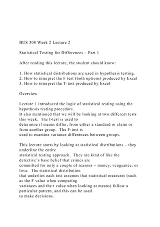
  • 1. BUS 308 Week 2 Lecture 2 Statistical Testing for Differences – Part 1 After reading this lecture, the student should know: 1. How statistical distributions are used in hypothesis testing. 2. How to interpret the F test (both options) produced by Excel 3. How to interpret the T-test produced by Excel Overview Lecture 1 introduced the logic of statistical testing using the hypothesis testing procedure. It also mentioned that we will be looking at two different tests this week. The t-test is used to determine if means differ, from either a standard or claim or from another group. The F-test is used to examine variance differences between groups. This lecture starts by looking at statistical distributions – they underline the entire statistical testing approach. They are kind of like the detective’s base belief that crimes are committed for only a couple of reasons – money, vengeance, or love. The statistical distribution that underlies each test assumes that statistical measures (such as the F value when comparing variances and the t value when looking at means) follow a particular pattern, and this can be used to make decisions.
  • 2. While the underlying distributions differ for the different tests we will be looking at throughout the course, they all have some basic similarities that allow us to examine the t distribution and extrapolate from it to interpreting results based on other distributions. Distributions. The basic logic for all statistical tests: If the null hypothesis claim is correct, then the distribution of the statistical outcome will be distributed around a central value, and larger and smaller values will be increasingly rare. At some point (and we define this as our alpha value), we can say that the likelihood of getting a difference this large is extremely unlikely and we will say that our results do not seem to come from a population that matches the claims of the null hypothesis. Note that this logic has several key elements: 1. The test is based on an assumption that the null hypothesis is correct. This gives us a starting point, even if later proven wrong. 2. All sample results are turned into a statistic that matches the test selected (for example, the F statistic when using the F-test, or the t-statistic when using the T-test.) 3. The calculated statistic is compared to a related statistical distribution to see how likely an outcome we have. 4. The larger the test statistic, the more unlikely it is that the result matches or comes
  • 3. from the population described by the null hypothesis claim. We will demonstrate these ideas by looking at the questions being asked in this week’s homework. We will show results of the related Excel tests, and discuss how to interpret the output. We need to remember that seeing different value (mean, variance, etc.) from different samples does not tell us that the population parameters we are estimating are, in fact, different. The one thing we know about sampling is that each sample will be a bit different. They generally provide a “close enough” estimate to the population values of concern for decision and action purposes. But, they are not an exact match. This difference is examined by the use of the statistical tests, which tell us how much importance we should attach to observed differences. Lecture Examples The lectures for each week will also look at our class question of whether or not males and females are paid equally for equal work. These additional analyses provide some different clues on what the data is trying to tell us about company pay practices. While your analysis will focus directly on the salary that males and females are being paid, the lecture examples will use an alternate method of examining pay practices. Many
  • 4. compensation professionals often use a relative pay measure called the “comparison-ratio,” or compa-ratio, to examine pay patterns within the company. Some background on this measure. Many companies use grades to group jobs of equal value to the company into groups that have a similar pay range – the values that a company is willing to pay employees for the job. (As strong as a performer a mail room clerk is, they will rarely be paid the same as the CEO.) Many companies will set the middle of this range, the midpoint, as the average salary that that market pays to hire someone into the job. This is how companies remain competitive in their hiring. Now, compensation professionals will generally want to analyze how the company is paying employees relative to these market rates (as summarized by the midpoint). One approach is to divide each employee’s salary by its related midpoint. The outcome is the compa-ratio which is considered an alternate measure of pay that eliminates the impact of different grades. The compa-ratio reports pay as a ratio of the actual salary divided by the salary grade’s midpoint. The compa-ratio shows if an employee is being paid more than the midpoint (measure’s value > 1.0) or less than the midpoint (< 1.0). This measure allows us to look at salary dispersion within a company without focusing on the exact dollar values. It allows a comparison between what the company is paying and what the outside market is paying (which most company’s target as the midpoint of a salary range) for the jobs.
  • 5. The compa-ratio shows if employees are paid above or below the grade midpoint and it can be used to see what the dispersion pattern of pay. Equal pay would expect to see similar distributions, variances and means, between males and females in this measure. The lecture examples will cover the same statistical tests as the homework assignments but will focus on the compa-ratio pay measure rather than salary. As such, the results presented each week should be included and/or factored into your weekly conclusions on what the data has told us about the answer to our question. The first step in looking at whether males and females are paid equally would be to look at the average pay of each. Given our sample is a random sample of the population of employees (and, therefore considered to be representative of the population), the average salaries or average compa-ratios (they measure related but not identical measures of pay) will give us an indication of whether things are the same for each gender or not. One issue in looking at averages is the variation within the groups. If both groups have the same or very similar variation across the salaries then we test the averages for a difference using one approach. If the group variances are significantly different, we use a slightly approach. So, the first step is to examine group variances. This
  • 6. is done with the F-test. F-test As noted, the F-test is used to compare variances to determine if the differences noted could be from simple sampling error (also known as pure chance alone) or if the differences are large enough to be considered statistically different. The F statistic is simply one group’s variance divided by the other group’s variance. (When done by hand, it is traditional to have the largest variance in the numerator, but this is not critical when Excel performs the test for us.) So, if the variances are equal, then the result of one variance divided by the other would equal 1.0 – this is the center of the F distribution. How about a situation where one variance equaled 4 and the other equaled 5 (randomly picked numbers for this example)? If we divided the larger by the smaller, we would get 5/4 = 1.25 while if we divided the smaller by the larger, we would get 0.8. Note that these values are on each side of the center value of 1.00. This is what is meant by “two tails” with the F-test – one tail of the distribution has values less than 1.0 while the other has values greater than 1.0.. Our value of F depends first on the variances (of course) and then on how we do the division. The likelihood of these two variances coming from populations that have the same variance does not depend upon which tail the result is in, but rather how likely it is to see a difference from 1.00. This is given to us by the F-test p-value (probability value of seeing a difference as large or larger than what we have if the null hypothesis is true).
  • 7. One new concept introduced with the F-test is the idea of degrees of freedom (df). While the technical explanation is somewhat tedious, we can understand the concept with a simple example. If we have 5 numbers, for example: 1, 2, 3, 4, and 5; we also have a sum of them; in this case 15. Now, assume we can change any of the numbers in the data set with the only requirement being that the total must remain the same. How many of the numbers are we free to change; or what is our degree of freedom in making changes? In this case, we can change any 4 of the values, as soon as we do so we automatically get the fifth value (whatever is needed to make the sum equal to 15). Thus, to generalize, our df is the count we have minus 1 (equaling n -1). N-1 is the formula for the degrees of freedom for each variable in the F-test. We will se this idea in other statistical tests, each of which has its own formula to calculate it. The nice thing is that Excel will give us this outcome without our needing to worry about it, and we rarely have to actually use it in any of our work – but, it is technically part of most statistical tests. There are two versions of the F-test available for use. One is located in the Data ribbon under the Analysis block in the Data Analysis link and is called F-Test Two-Sample for Variances. The other is located in the Fx Statistical list (which is duplicated in the Formulas ribbon under the More Functions option and the Statistical list) and is called simply F.test.
  • 8. While both test variances, there is an important difference. The F-Test Two Sample for Variances option provides some additional summary statistics (mean, variance, count) for each sample, but only provides a one-tail test outcome. One-tail results, whether with the F-Test or the T-test are used to test a directional difference in variances, when we want to know if one variance is larger (or smaller) than the other. Since, in general we are interested in the simpler question of whether the variances are equal or not (without regard to which is larger), when using this form to test for equality or not, we need to double the p-value to find the two t-tail p- value we need for our decision on rejecting the null hypothesis. On the other hand, the F.test found in Fx or Formulas returns only the two-tail p-value; enough for a decision on rejecting or failing to reject the null hypothesis of no difference but nothing else. Technically, this is the version we should use when conducting our two-tail questions in the homework, but (as noted) either can be used if we remember to double the p- value for the one -tail outcome. Example: Testing for Variance Equality As mentioned above, it is often beneficial to start with looking at variance equality when comparing groups. We need to start our analysis of equal pay for equal work by seeing if there is even an issue to be concerned with. So, we have selected our random sample of 25 males and 25 females from our corporate population. (A couple of
  • 9. assumptions; the company exists in only one location, and all our employees in the sample are exempt professions or managers with at least a bachelor’s college degree.) Our initial question is: Are the male and female compa-ratio variances equal? (Note, if they are, this would mean that the standard deviations of both groups are the same.) As with all statistical tests, we will be using our samples to make judgements or inferences about the population values. While the sample result values will differ, this difference may not be large enough to show that the population values are not the same. Question 1. One of the first things of interest to detectives is if the behavior of the suspects differs from what they normally do. That is, who’s behavior varies from the norm? Relating this to our compa-ratio measures has us asking if the compa-ratio variance for males and females are equal within the population. (In the homework, the question asks about salary variances. The logic and approach for answering the salary- based question is the same as shown below.) Variance equality is tested using the F-Test. There are two versions of this test available to us that we could use, and both will be shown below. Note that equal standard deviations do not automatically mean that the means are close, it just tells us if the dispersion patterns are
  • 10. similar. If similar, the means of each group can be considered equally reflective of the data. The following focuses on just setting up the data for and performing the statistical test. The following show only the output for the six hypothesis testing steps. How the Excel F-tests are set up is covered in Lecture 3 for this week. Step 1: The question asked is whether the variances for males and females are equal. The hypothesis statements for an equality test are shown below. Ho: Male compa-ratio variance = Female compa-ratio variance Ha: Male compa-ratio variance =/= Female compa-ratio variance (Since the question asks about equality and not a directional difference, this is a two-tail test. The Null must contain the names of the two variables involved (Male and Female), the statistic being tested (variance), and the relationship sign (=). The alternate provides the opposite view so that between them all possible outcomes are covered. We are only concerned if the variances are equal, not whether one or the other is larger (or smaller).) Step 2: We state our decision-making criteria here. It is: Alpha = 0.05 (This will be the same for all statistical tests we perform in the class, and therefore the same in all hypothesis set-ups.) Step 3: The test, test statistic, and the reason for selecting the
  • 11. test are stated here. For this example, we are using: F statistic and F-test for Variance. We use these as they are designed to test variance equality. Step 4: Our decision-making rule is presented here: Reject the null hypothesis if the p- value is < alpha = 0.05. (This step is also the same for every statistical test we will perform; it says we will reject the null hypothesis if the probability of getting a result as large as what we see is less than 5% or a probability of 0.05.) Note that these steps are set-up before we even look at the data. While, we may have set up the data columns, we should not have done any analysis yet. These steps tell us how we will make a decision from the results we get. Step 5: Perform the analysis. This is the step where Excel performs the analysis and produces output tables. The setting up of each Excel test is covered in Lecture 3, we are primarily interested in how to interpret the results in this lecture. Here is a screenshot of the results for both versions of the F- test. (Only one is needed for the question.) Step 6: Conclusions and Interpretation. This is where we
  • 12. interpret what the data is trying to tell us. Before moving on to interpreting these results, let’s look at what we have. The F-Test Two-Sample for Variances output clearly has more information than the F.TEST. We have the labels identifying each group as well as the mean, variance, and count (Observations) for each group. The df, equaling the (sample size -1), is shown as well as the calculated F statistic (which equals the left group’s (or Male in this case) variance divided by the right group’s (Female) variance. Note, Excel divides the variances in the order that they were entered into the data entry box, for this example the Males were entered first. The next two rows are critical for our decision making; but they are incomplete. They show the one-tail critical values used in decision making. The P(F<=f) one-tail is the P- value, or the probability of getting an F-value as large or larger than we have if the null hypothesis is true. However, it is only a one-tail outcome, while we want a two-tail outcome, since we only care about the variances being equal or not, not which one is larger. So, the result as presented cannot be used directly. What we need to do will be covered after we look at the F.TEST result.
  • 13. The F.TEST gives less information, but it provides us with exactly what we need; the two-tail p-value. For our data set, we have a 40% (rounded) chance of getting an F value this large or larger purely by chance alone when we are looking at a two-tail outcome. Note that this value, 0.39766 is twice the one-tail value of 0.19883 from the F-Test table. This will always be true, the two-tail probabilities will be twice the one-tail values. So, if we want to use the F-TEST Two-Sample for Variance tool, we need to double the p-value before making our step 6 decisions. We are now ready to move on to what step 6 asks for. This step has several parts. • What is the p-value: 0.3977 (our compa-ratio example result). This value equals EITHER tht F.TEST outcome or 2 times the F-test result. (If, the F-test p-value is in cell K-15, you could enter =2*K15 to get the value desired). • What is your decision: REJ or Not reject the null? (If our p- value is < (less than) 0.05, we say REJ, if the p-value is > (larger than) 0.05, we say NOT reject. This is what our decision rule says to do.) Our answer is for compa- ratio variances: NOT Rej. This means we do not reject the claim made by the null hypothesis and accept it as the most likely description of the variances within the population. • Why? This line asks us to explain why we made the decision
  • 14. we did. Our compa- ratio response is: The p-value is > (greater than) 0.05, and the decision rule is reject if the p-value was < 0.05. (The answer here is simply why, based on the reasoning shown above, you chose your REJ or NOT Rej choice.) • What is your conclusion about the variances in the population for the male and female salaries? This part asks us to translate the statistical decision into a clear answer to the initial question (Are male and female compa- values equal?) Our response: We do not have enough evidence to say that the variances differ in the population. The variances are equal in the population. Had we rejected the null hypothesis, we would have said the population variances differed. Note that this question did not tell us anything about actual pay differences between the genders. It did tell us that both groups are dispersed in a similar manner, and thus supported some of the conclusions we drew from looking at the data last week. Examples: Testing for Mean Equality While we test for variance equality with an F test, we use the T- Test to test for mean equality testing. The t-test also uses the degree of freedom (df) value in providing us with our probability result; but again, Excel does the work for us. The t distribution is a bell-shaped curve
  • 15. that is flatter and a bit more spread out than the normal curve we discussed last week. The center is located at 0 (zero) and the tails (the negative and positive values) are symmetrical. The t statistic for the testing of two means is basically: (Mean1 – Mean2)/standard error estimate. (The standard error formula varies according to which type of t-test we are performing.) Note that the t will be either positive or negative depending upon which mean is larger. So, if we are interested in simply equal or not equal, it does not matter if we have a positive or negative t value, only the size of the difference matters. As with the F-test, half of our alpha goes in the positive tail and half goes in the negative tail when making our equality decision. We have two questions about means this week. Question 2. The second question for this week asks about salary mean equality between males and females. Again, the set up for this question is covered in Lecture 3, we are concerned here with the interpretation of the results. (Note, the comments about each step made above apply to this example as well, but they will not be repeated except for specific information related to the t- test outcome.) Specific differences from the variance example of question 1 will be highlighted with italics. Again, the results discussed with each step are shown in Lecture 2.
  • 16. Since the question asks if male and female compa-ratios (salaries in the homework), are equal we have a equal versus non-equal hypothesis pair. Step 1: Ho: Male compa-ratio mean = Female compa-ratio mean Ha: Male compa-ratio mean =/= Female compa-ratio mean Step 2: The decision criteria is constant: Alpha = 0.05 Step 3: t statistic and t-test, assuming equal variances. We use these as they are designed to test mean equality, and we are assuming (and according to the F-test have) equal variances. Step 4: Again, our decision rule is the same: Reject the null hypothesis if the p-value is < alpha = 0.05. Step 5: Perform the analysis. Here is the screen shot for the results, using the same data as with Question 1. As with the F-test output, the t-test starts with the test name, the group names, and some descriptive statistics. Line 4 start with a new result, the Pooled Variance; this is a weighted average of the sample variances since we are assuming that the related population variances are equal. The next line, hypothesized Mean Difference, shows up only if a value was entered in the data input box setting up the
  • 17. test (discussed in Lecture 3). Next comes our friend degrees of freedom, which equal the sum of both sample sizes minus 2 (or N1-1 + N2 -1). The calculated T value (similar to the calculated F value in the F test output) comes next. Note that since we have a negative t Stat, it falls in the left tail of the t distribution. This is important in one tail tests but not in two tail tests. Following the calculated T value come the one and two tail decision points. The one tail p-value is found in the P(T<==t) one-tail row followed by the T critical one-tail value. The two tail results follow. Step 6: Conclusions and Interpretation. This step has several parts. What is the p-value? 0.571 (our rounded compa-ratio example result). (Since we again have a two-tail test, we use the P(T<=t) two- tail result.) What is your decision: REJ or Not reject the null? NOT Rej (our compa-ratio result) Why? The p-value (0.571) is > (greater than) 0.05. (The compa- ratio result) What is your conclusion about the means in the population for the male and female
  • 18. salaries? We do not have enough evidence to say that the means differ in the population. So, our conclusion is that the means are equal in the population. (Our compa-ratio result.) Question 3 The third question for this week asks about salary differences based on educational level rather than gender. Since education is a legitimate reason to pay someone more, it will be helpful to see if a graduate degree results in a higher average pay. Note that this question has a directional focus (do employees with an advanced degree (degree code = 1) have higher average salaries?). This means we must develop a direction set of hypothesis statements. We will use the terms UnderG (for undergraduate degree code 0) and Grad (for graduate degree code 1) in these statements. Again, the results discussed with each step are shown in Lecture 2. Step 1: Ho: UnderG mean compa-ratio => Grad mean compa- ratio Ha: UnderG mean ratio < Grad mean compa-ratio (Note the way the inequalities are set up; since the question is if degree 1 salary means >, the question becomes the alternate hypothesis as it does not contain an = claim. These can be written with the Grad mean listed first but the arrow heads must point to Grad showing an expectation that grad means are larger.)
  • 19. Step 2: Alpha = 0.05 (Our constant decision criterion) Step 3: t statistic and t-test assuming equal variances. We use these as they are designed to test mean equality. (The variance equality assumption is part of the question set-up.) Step 4: Reject the null hypothesis if the p-value is < alpha = 0.05. (Our constant decision rule.) Step 5: Perform the analysis. Here is a screen print for a T-test on the question of whether the graduate and undergraduate degree compa-ratios means in the population are equal or not. We are assuming equal variances, we are using the T-Test Two-Sample Assuming Equal Variances form. t-Test: Two-Sample Assuming Equal Variances UnderG Grad Mean 1.05172 1.07324 Variance 0.00581 0.005999 Observations 25 25 Pooled Variance 0.005904 Hypothesized Mean Difference 0 df 48
  • 20. t Stat -0.99016 P(T<=t) one-tail 0.163529 t Critical one-tail 1.677224 P(T<=t) two-tail 0.327059 t Critical two-tail 2.010635 The table output is read exactly the same way as with the question 2 table with the exception that we are interested in the one-tail outcome, so we use the (highlighted) one- tail p-value row in our decision making. Step 6: Conclusions and Interpretation. This step has several parts. • What is the p-value? 0.164(rounded) (our rounded compa-ratio example result). (Since we again have a one-tail test, we use the P(T<=t) one-tail result.) • Is the t value in the t-distribution tail indicated by the arrow in the Ha claim? Yes. The t-value is negative, and the Ha arrow points to the left (or negative) tail of the t distribution. (Since we only care about a difference in one direction, the result must be consistent with the desired direction. Only large negative values are of interest in this case/set-up, since our difference is calculated by (UnderG – Grad); large negative values show a larger Grad salary. If we had said Grad <= Underg in the Null, the alternate arrow would have pointed to the right or positive
  • 21. tail, and a positive t would have been needed.) • What is your decision: REJ or Not reject the null? NOT Rej (our compa-ratio result) • Why? The p-value is > (greater than) 0.05. So, the sign does not matter in this case, but it is in the correct or negative tail. (The compa-ratio result) • What is your conclusion about the impact of education on average salaries? We do not have enough information to suggest that graduate degree holders have a higher average salary than undergraduate degree holders. (Our compa-ratio result.) Question 4 While the week 1 salary results suggest that males and females are not paid the same, this week’s compa-ratio tests still do not suggest any inequality. Gender Compa-ratio variances and means are not significantly different. A somewhat surprising result was that graduate degree holders did not have higher compa-ratios. We still cannot answer our equal pay for equal work question; however, as we have yet developed a measure of pay for equal work. Compa-ratios do remove the impact of grades, but too many other work-related variables still need to be examined.
  • 22. Summary The F and t tests are used to determine if, based upon random sample results, the population parameters can reasonably be said to differ. The F- test looks for differences in population variances, while the t-test examines population mean differences. Both tests are performed as part of the hypothesis testing procedure and always is done in step 5. Differences in sample results can be transformed into statistical distributions that allow us to determine the probability or likelihood of getting a difference as large or larger than we found. It is this transformation that allows us to make our decisions about the differences we see in the results. When either test is set-up using the Data | Analysis toolpak function, these tests will provide summary sample descriptive statistics for the mean, variance, and count as well as the calculated statistic, the critical value of the statistic, and the p- value. When set-up using Excel’s Fx or Formula functions, only the p-value is returned. For both tests, if the appropriate p-value is less than the specified alpha (always 0.05 in this class), we reject the null hypothesis and say the alternate is the more likely description of the population. We can test for a simple difference (called a two-tail test) where it does not matter which
  • 23. group has the larger value or we can use a directional test (called a one-tail test) where we are concerned about which variable is larger (or smaller). The null and alternate hypothesis define which difference we are looking for. The t-test has three versions: equal variances, unequal variances, and paired. The paired test is used when we have two measures on each subject (such as the salary and midpoint for each employee). The F-test is used to help us decide if we need to use the equal or unequal variance form of the t-test. The Analysis toolpak F test defaults to a one-tail test so we need to double its p-value when testing for simple variance differences. The Fx (or Formula) F-test lets us select a one- or two-tail outcome. Please ask your instructor if you have any questions about this material. When you have finished with this lecture, please respond to Discussion Thread 2 for this week with your initial response and responses to others over a couple of days. N4685 Capstone
  • 24. Capstone Reflective Journal Submit by 2359 CST Saturday of each module specified in Course Calendar. Name: Date: Overview: Capstone Reflective Journal Each module you will make an entry into your Journal. You are asked to reflect on 3 of the key points for each module. Each entry should reflect on your understanding of the topic, your experiences and observations in your work environment or general nursing environment regarding the module topic. This is a cumulative document. You will save it to your own computer desktop or memory device and update it each week. You may choose to record more than one entry each week, especially if you have an “aha!” moment as a result of your reading, discussions, or experience. You will upload and submit the latest version of your Capstone Reflective Journal to Blackboard by 2359 the Saturday following each of the first six modules of this course. It is not necessary that your entries be formatted or written in any particular way because it is for your benefit. Your entries will only be reviewed to ensure that you are making sufficient progress and thinking deeply about the requirements in the course. RubricsUse this rubric to guide your Journal entries. There will be total of 6 Journal entries for Modules 1-6. Each Module you are expected to address 3 key points from the Module content, discuss how each point applies to your practice as a nurse, and, finally, how will your practice change in the future because of this information. In Module 7 your Journal entries will be used as you write the last paper for the program, the Synthesis Paper. Journal Rubric for each Module Criteria
  • 25. Target Unacceptable Address 3 Key Points from Module for each Journal entry (50 points) Discuss the 3 key points selected and why they are important or memorable. (50 points) Does not sufficiently record connections or reflections (0 Points) Relevance and Evidence Based Practice (25 points) Connect RN-BSN experiences from each key point to career goals, prior nursing practice, a previous RN BSN course, nursing theories or research. Cite and reference as necessary. (25 points) Fails to connect RN-BSN experiences to goals, prior nursing practice, coursework, theories or research to key areas addressed or no references. (0 points) Future (25 points) Describes how personal practice will be different in the future
  • 26. based on RN-BSN program as a result of the 3 key areas addressed. (25 points) Fails to describes how personal practice will be different in the future based on RN-BSN program (0 points) Late submissions will be penalized 5% per day unless prior arrangements have been made with your Academic Coach to complete the assignment at a later time. Instructions Each week, record your experiences, connections to your course goals, and reflections as they relate to the given prompts and/or your course project. You must record one entry each week, but may record more (insert rows as needed). You may find it helpful and rewarding to record one entry at the beginning of the week, think about the prompt during the week, then record another at the end of the week. For privacy, refer to patients, online colleagues, and/or co-workers with initials instead of names. Save this document to your own computer desktop or storage device after each entry to create a cumulative journal. You will upload the document and submit it each week by 0800 CST Friday following the course week. (You will not submit your Reflective Journal for Week 5 entries, but may continue to record entries for your own purposes.) Remember that the more thoughtfully and intentionally you record your immediate reflections, the easier it will be for you to pull all your experiences and thoughts together for your Journal Paper in Week 5. Module Journal Entries
  • 27. A separate Journal entry is required for Modules 1-6 by 2359 Saturday of each indicated module. Provide details of your thinking, including insights, challenges, paradigm shifts, and goals. Identify previous course topics, readings, or research that relate to the prompt. Journal Entry Module 1: Identify 3 key points form this module. Reflect on how why each point is important, how it impacts on your work experience or nursing practice, and how will you change your practice in the future based on each key area. Key Point 1 Key Point 2 Key Point 3 Module 2: Identify 3 key points form this module. Reflect on how why each point is important, how it impacts on your work experience or nursing practice, and how will you change your practice in the future based on each key area. Key Point 1 Key Point 2 Key Point 3 Module 3: Identify 3 key points form this module. Reflect on how why each point is important, how it impacts on your work experience or nursing practice, and how will you change your practice in the future based on each key area. Key Point 1 Key Point 2
  • 28. Key Point 3 Module 4: Identify 3 key points form this module. Reflect on how why each point is important, how it impacts on your work experience or nursing practice, and how will you change your practice in the future based on each key area. Key Point 1 Key Point 2 Key Point 3 Module 5: Identify 3 key points form this module. Reflect on how why each point is important, how it impacts on your work experience or nursing practice, and how will you change your practice in the future based on each key area. Key Point 1 Key Point 2 Key Point 3 Module 6: Identify 3 key points form this module. Reflect on how why each point is important, how it impacts on your work experience or nursing practice, and how will you change your practice in the future based on each key area. Key Point 1 Key Point 2 Key Point 3
  • 29. Module 7: Identify 3 key points form this module. Reflect on how why each point is important, how it impacts on your work experience or nursing practice, and how will you change your practice in the future based on each key area. Key Point 1 Key Point 2 Key Point 3 ©2015University of Texas at Arlington Page 1 of 5