Week 2 – Lecture 3 Making judgements about differences between group statistics is one of the most powerful things that statistics can do for us. It is also one of the most counter-intuitive things that we need to master in the class. Lecture 1 introduced the hypothesis testing procedure used in statistical testing. Lecture 2 examined how to set up, perform, and interpret the F test for variance equality. This lecture will focus on t-tests for testing mean equality. Again, these examples will use the compa-ratio variable, while the homework should use the Salary variable. The T-Test While we test for variance equality with an F test, we use the T-Test to test for mean equality testing. The t-test also uses the degree of freedom (df) value in providing us with our probability result; but again, Excel does the work for us. There are three versions of the T-Test done for us by Excel. The first two are similar except one version is done if the variances are equal and the other if the variances are not equal. (Now we see the second reason for performing the F-test first.) The third version of the T-test is for paired data, and is called T-test Paired Two Sample for Means. Paired data are two measures taken on the same subject. Examples include a math and English test score for students, preference for different drinks, and, in our data set the salary and midpoint values. Note that paired data must be measured in the same units, and be from the same subjects. Students in the past have incorrectly used the paired t-test on male and female salaries. These are not paired, as the measures are taken on different people and cannot be paired together for analysis. In many ways, setting up Excel’s T-tests, and virtually all the functions we will study, follow the same steps as we just went through: 1. Set up the data into distinct groups. 2. Select the test function from either the Fx or Analysis list 3. Input the data ranges and output ranges into the appropriate entry boxes, checking Labels if appropriate. 4. Clicking on OK to produce the output. As with the F-test, the T-test has a couple of options depending upon what you want your output to look like. The Fx (or Formulas) option returns simply the p-value for the selected version of the test. The Data | Analysis selection provides descriptive statistics that are useful for additional analysis (some of which we will discuss later in the course). The t-test requires that we select between three versions, one assuming equal variances between the populations, one assuming unequal variances in the populations, and one requiring paired data (two measures on each element in the sample, such as salary and midpoint for each person in our data set.) All have the same data set-up approach, so only one will be shown. Question 2 The second question for this week asks about salary mean equality between males and females. The data and test se.

1. Week 2 – Lecture 3
Making judgements about differences between group statistics
is one of the most
powerful things that statistics can do for us. It is also one of
the most counter-intuitive things
that we need to master in the class.
Lecture 1 introduced the hypothesis testing procedure used in
statistical testing. Lecture
2 examined how to set up, perform, and interpret the F test for
variance equality. This lecture
will focus on t-tests for testing mean equality. Again, these
examples will use the compa-ratio
variable, while the homework should use the Salary variable.
The T-Test
While we test for variance equality with an F test, we use the T-
Test to test for mean
equality testing. The t-test also uses the degree of freedom (df)
value in providing us with our
probability result; but again, Excel does the work for us.
There are three versions of the T-Test done for us by Excel.
The first two are similar
except one version is done if the variances are equal and the
other if the variances are not equal.
(Now we see the second reason for performing the F-test first.)
The third version of the T-test is for paired data, and is called
T-test Paired Two Sample

2. for Means. Paired data are two measures taken on the same
subject. Examples include a math
and English test score for students, preference for different
drinks, and, in our data set the salary
and midpoint values. Note that paired data must be measured in
the same units, and be from the
same subjects. Students in the past have incorrectly used the
paired t-test on male and female
salaries. These are not paired, as the measures are taken on
different people and cannot be paired
together for analysis.
In many ways, setting up Excel’s T-tests, and virtually all the
functions we will study,
follow the same steps as we just went through:
1. Set up the data into distinct groups.
2. Select the test function from either the Fx or Analysis list
3. Input the data ranges and output ranges into the appropriate
entry boxes, checking
Labels if appropriate.
4. Clicking on OK to produce the output.
As with the F-test, the T-test has a couple of options depending
upon what you want your
output to look like. The Fx (or Formulas) option returns simply
the p-value for the selected
version of the test. The Data | Analysis selection provides
descriptive statistics that are useful for
additional analysis (some of which we will discuss later in the
course).
The t-test requires that we select between three versions, one
assuming equal variances
between the populations, one assuming unequal variances in the

3. populations, and one requiring
paired data (two measures on each element in the sample, such
as salary and midpoint for each
person in our data set.) All have the same data set-up approach,
so only one will be shown.
Question 2
The second question for this week asks about salary mean
equality between males and
females. The data and test set-up were discussed in Lecture
two. Here is how we set up the
steps for this question using compa-ratio as our example.
(Note, the comments about each step
made in the variance example above apply to this example as
well, but they will not be repeated
except for specific information related to the t-test outcome.)
Specific differences from the
variance example of question 1 will be highlighted with italics.
Again, the results discussed with
each step are shown in Lecture 2.
Step 1: Ho: Male compa-ratio mean = Female compa-ratio mean
Ha: Male compa-ratio mean =/= Female compa-ratio mean
Step 2: Alpha = 0.05
Step 3: t statistic and t-test, assuming equal variances. We use
these as they are designed to test
mean equality, and we are assuming equal variances.
Step 4: Reject the null hypothesis if the p-value is < alpha =
0.05.

4. Step 5: Perform the analysis. This step provides the cell
location to place your results in, K35 for
this question.
Setting up the data and test for question 2 about mean equality
is similar to what one for the F-
test question, and we can actually use the same data columns as
we used in question 1 on
variances. Again, after sorting the data into your comparison
groups (with labels as we did for
the F-test), select the appropriate test from either the Fx or
Analysis list. A completed T-test
Two-Sample Assuming Equal Variances input table is shown
below.
The input box looks a lot like the one we saw for the F-test, and
is completed in the same way.
Enter the data ranges in the same order you have them listed in
the hypothesis statements, check
the labels box if appropriate, and identify your output range top
left cell (this is given in the
homework problems for a consistent format for instructor
grading).
There is one input that differs and which we have not discussed,
Hypothesized Mean Difference.
For the most part, we do not use this. An example of when we
might want to is when we have
made a change and want to test its effectiveness. For example,
we might have a pre- and post-
test in a training course. In the original design, the average
improvement might be 10 points on

5. the post-test. If we change the design of the training, we would
be interested not only in showing
a significant change between the two tests but also a better
change due to the revision. In this
case, the first 10-point difference in the tests is a given, we
want to know if the additional score
change is significant. So, we enter 10 in the HMD box, and the
analysis looks at only the mean
difference larger than 10, the marginal improvement due to the
design change.
The input for the Fx T.Test contains 4 boxes, and produces the
p-value in the cell the cursor is in.
The first two boxes are the data range for each variable, and
these should not have a label
included. The third box asks whether you have a one or two tail
test. The forth box asks
for the kind of test, paired, equal variance, or unequal variance.
Once we click OK for the T.test. we get a output, the p-value.
When we click OK on the Analysi
ToolPak function we get a more descriptive table; much like the
differences with the two
versions of the F. Here is a screen print for question 2 in this
week’s homework. The question
in the homework is about the equality of male and female
salaries. For this example, we will
look at the equality of male and female compa-ratios. Since we
found (above) that the variances
were not statistically different in the population, we will use the
equal variance version of the 2-
sample t-test.
Here is the screen shot for the result of the above data entry for
a test about equal compa-ratio

6. means for males and females.
As with the F-test output, the t-test starts with the test name, the
group names, and some
descriptive statistics. Line 4 start with a new result, the Pooled
Variance; this is a weighted
average of the sample variances since we are assuming that the
related population variances are
equal. The next line, hypothesized Mean Difference, shows up
only if a value was entered in the
data input box setting up the test.
Next comes our friend degrees of freedom, which equal the sum
of both sample sizes minus 2 (or
N1-1 + N2 -1). The calculated T value (similar to the
calculated F value in the F test output)
comes next. Note that since we have a negative t Stat, it falls in
the left tail of the t distribution.
This is important in one tail tests but not in two tail tests.
Following the calculated T value come
the one and two tail decision points. The one tail p-value is
found in the P(T<==t) one-tail row
followed by the T critical one-tail value. The two tail results
follow.
Step 6: Conclusions and Interpretation. This step has several
parts.
What is the p-value? 0.571 (our rounded compa-ratio example
result).

7. (Since we again have a two-tail test, we use the P(T<=t) two-
tail result.)
What is your decision: REJ or Not reject the null? NOT Rej
(our compa-ratio result)
Why? The p-value (0.571) is > (greater than) 0.05. (The compa-
ratio result)
What is your conclusion about the means in the population for
the male and female
salaries? We do not have enough evidence to say that the means
differ in the population.
The means are equal in the population. (Our compa-ratio
result.)
Question 3
The third question for this week asks about salary differences
based on educational level
rather than gender. Here is how we set up the steps for this
question using compa-ratio as our
example. (Note, the comments about each step made in the
variance example above apply to
this example as well, but they will not be repeated except for
specific information related to the t-
test outcome.)
Note that this question has a directional focus (do employees
with an advanced degree
(degree code = 1) have higher average salaries?). This means
we must develop a direction set of
hypothesis statements. We will use the terms UnderG (for

8. undergraduate degree code 0) and
Grad (for graduate degree code 1) in these statements. Again,
the results discussed with each
step are shown in Lecture 2.
Step 1: Ho: UnderG mean compa-ratio => Grad mean compa-
ratio
Ha: UnderG mean ratio < Grad mean compa-ratio
(Note the way the inequalities are set up; since the question is
degree 1 salary means >,
the question becomes the alternate hypothesis as it does not
contain an = claim. These
can be written in other ways, but must have the alternate
relating to the question asked.)
Step 2: Alpha = 0.05
Step 3: t statistic and t-test assuming equal variances. We use
these as they are designed to test
mean equality. (The variance equality assumption is part of the
question set-up.)
Step 4: Reject the null hypothesis if the p-value is < alpha =
0.05.
Step 5: Perform the analysis. This step provides the cell
location to place your results in, K60 for
this question (I60 for compa-ratio example). Except for using
Degree as the sorting group
variable, the data set-up for the third question is the same as
done in question 2, so no new screen
shot is needed.
Here is a screen print for a T-test on the question of whether the

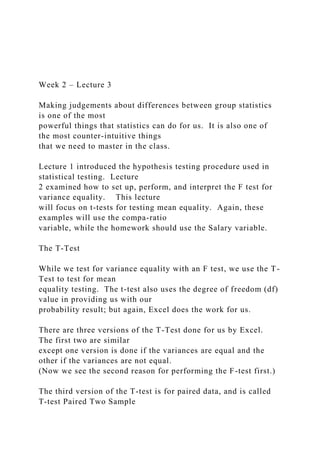
9. graduate and undergraduate
degree compa-ratios means in the population are equal or not.
We are assuming equal variances,
we are using the T-Test Two-Sample Assuming Equal Variances
form.
t-Test: Two-Sample Assuming Equal Variances
UnderG Grad
Mean 1.05172 1.07324
Variance 0.00581 0.005999
Observations 25 25
Pooled Variance 0.005904
Hypothesized Mean
Difference 0
df 48
t Stat -0.99016
P(T<=t) one-tail 0.163529
t Critical one-tail 1.677224
P(T<=t) two-tail 0.327059
t Critical two-tail 2.010635
The table output is read exactly the same way as with the
question 2 table with the exception that
we are interested in the one-tail outcome, so we use the
(highlighted) one-tail p-value row in our
decision making.

10. Step 6: Conclusions and Interpretation. This step has several
parts.
What is the p-value? 0.164(rounded) (our rounded compa-ratio
example result).
(Since we again have a one-tail test, we use the P(T<=t) one-tail
result.)
Is the t value in the t-distribution tail indicated by the arrow in
the Ha claim? Yes. The t-
value is negative, and the Ha arrow points to the left (or
negative) tail of the t
distribution.
(Since we only care about a difference in one direction, the
result must be consistent with
the desired direction. Only large negative values are of interest
in this case, since our
difference is calculated by (UnderG – Grad); large negative
values show a larger Grad
salary.)
What is your decision: REJ or Not reject the null? NOT Rej (our
compa-ratio result)
Why? The p-value is > (greater than) 0.05. So, the sign does
not matter in this case, but
it is in the correct or negative tail. (The compa-ratio result)
What is your conclusion about the impact of education on
average salaries? We do not
have enough information to suggest that graduate degree holders
have a higher average
salary than undergraduate degree holders. (Our compa-ratio
result.)

11. Special Case: The One-Sample T-test
Often, we may want to test the results of a sample against a
standard; for example, is the
weight of a production run of 8 ounces of canned pears actually
equal to the standard of 8.02 oz.?
(Note, most manufactures will put in slightly more than the
label says to avoid being
underweight which could result in a fine.)
Excel is not set up to perform this test, but we can “trick” it to
do this for us. In the one-
sample case, we need two pieces of information, the sample
values and our comparison standard.
Set these up as if they were any two-sample data sets, have our
sample values (for example, 25
female compa-ratios in one column) and our comparison value
in another. The comparison data
column will only contain a single value equal to our comparison
value. For example, we might
want to test if the average female compa-ratio was greater than
the compa-ratio midpoint of 1.00.
The null would be H0: female compa-ratio mean <= 1.00 while
the alternate would be Ha:
Female compa-ratio mean > 1.00. The Compa-ratio data column
would contain the Female
compa-ratios and the other column (named for convenience as
Ho Data) would contain only the
value of 1.00, our standard value.
While we will leave the math for any interested student to
perform, if we take the T-test
unequal variance formulas for both the t-value and the df value

12. and have a variance of 0 for one
variable, both will reduce to the one-sample t-test formula and
df value. Knowing this, we can
use the unequal variance version of the t-test to perform what is
essentially a one-sample test for
us. Here is a screen shot of the data set-up and the t-test set-up
window.
The output of this test will show a mean of 1.0 and a variance of
0 for the Ho Data
(comparison) value, and the correct values for the Female
compa-ratio variable, including the p-
values.
Here is a video on setting up and using the t-test in Excel:
https://screencast-o-
matic.com/watch/cb6lYcImnn
Question 4
The forth question asks us to consider our findings. For the
homework, you need to
consider both the results found in the lectures as well as the
results from your analysis of the
salary data.
For our compa-ratio findings, it does not appear that the Equal
Pay Act is being violated.
From the sample of employees, it appears that males and
females are being paid about the same
relative to their grade midpoints across the grades. Last week
showed about equal means and
variances between the two groups, and this was confirmed with
the

13. Please ask your instructor if you have any questions about this
material.
When you have finished with this lecture, please respond to
Discussion thread 3 for this
week with your initial response and responses to others over a
couple of days before reading the
third lecture for the week.
https://screencast-o-matic.com/watch/cb6lYcImnn
https://screencast-o-matic.com/watch/cb6lYcImnn
Microeconomics – IndividualAssignment
By Prof. H. Schüller
Question 1
After a major earthquake struck Los
Angeles in 1994, several stores raised
the priceof
milk to over $6 per gallon. The local authorities
announced that they would investigate
and that they would enforce a law prohibiting
priceincreases of more than 10% during
emergency period. What is the likely effect
of such a law?
Question 2
Is it possible that an outright ban on foreign

14. imports will have no effect on the
equilibrium price?
Question 3
Arthur spends his income on bread and
chocolate.He views chocolate as good but is
neutral about bread, in that he does not care if
he consumes it or not. Draw his
indifference curve map.
Question 4
Sofia will consume hot dogs only with fries. Draw
her indifference curve map.
Question 5
Don spends his money on food and operas. Foodis
an inferior good for Don. Does he
view an opera performance as an inferior or
normal good? Explain why.
Question 6
Prescott (2004) argues that US employees work
50% more than German, French, and
Italian employees because they face lower
marginal tax rates. Assuming that workers in
all four countries have the same tastes toward leisure
time and goods, must it
necessarily be true that US employees will work

15. longer hours? Explain why. Does
Prescott’s evidence indicate anything about the relative
sizes of the substitution and
income effects? Why or why not?
Question 7
What is the long-run welfare effect of a
profit tax (the government collects a
specified
percentage of a firm’s profit) assessed on
each competitive firm in a market?
Question 8
Can a firm be a natural monopoly if it has a
U-shaped average cost curve? Why or why
not?
Question 9
Many universities provide students from low-income
families with scholarships,
subsidised loans, and otherprograms so that they
pay lower tuitions than students from
high-income families. Explain why universities behave
that way.
Question 10

16. Spencer’s Superior Stoves advertises a one-day sale on
electronic stoves. The ad
specifies that no phone orders are accepted and
that the purchaser must transport the
stove. Why does the firm include theserestrictions?
Question 11
Youruniversity is considering renting space in
the student union to one or two
commercial textbook stores. The rent the university
would charge depends on the profit
(before rent) of the store or stores and hence on
whether thereis a monopoly or a
duopoly. Which number of stores is better
for the university in terms of rent?Which
option is better for the students? Explain why.
Question 12
Will the pricebe lower if duopoly firms set
priceor if they set quantity? Under what
conditions can you give a definitive answer to
this question?
------------------------------
Enjoy!

17. Sheet1Visitors per week (k)Cost of hosting per week
(€)1.20101.902.00120.843.60117.693.20129.746.00150.527.201
59.428.40168.338.00146.649.00163.0012.00172.9611.00166.38
9.60167.2013.00191.0016.80217.6018.00239.5612.80200.9813.
60195.2021.60266.2715.20194.0224.00284.0816.80204.5426.40
267.7127.60293.2028.80301.6025.00275.0020.80260.1927.0029
9.9833.60306.9829.00267.9036.00274.4824.80297.6525.60298.
5039.60295.6027.20266.2142.00280.1243.20317.1529.60302.74
30.40286.4046.80320.9740.00278.24
Sheet2
Sheet3