Perfect competition SFLS

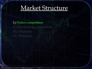
1. I.) Perfect competition
II.) Monopolistic competition
III.) Oligopoly
IV.) Monopoly
Market Structure

2. Market Structure
Models – a word of warning!
- Market structure deals with a number of economic
‘models’
- These models are a representation of reality to
help us to understand what may be happening in
real life
- There are extremes to the model that are unlikely
to occur in reality
- They still have value as they enable us to draw
comparisons and contrasts with what is observed
in reality 比较和对比什么是现实
- Models help therefore in analysing and evaluating
– they offer a benchmark 基准

3. - Even with these warnings, they do help
describe important concerns that you deal with
everyday you interact in any economic way:
-Degree of competition affects the consumer
will it benefit the consumer or not?
- Impacts on the performance and behaviour of
the company/companies involved.
Market Structure

4. We will start with the
structure that my vegetable
lady works in…

5. I.) Perfect competition
II.) Monopolistic competition
III.) Oligopoly
IV.) Monopoly
Market Structure

6. Profit = Total revenue – Total cost
the amount a
firm receives
from the sale
of its output
the market
value of the
inputs a firm
uses in
production
What is the goal of business?
We assume that the firm’s goal is to maximize profit.
But first we have to finish this,
I didn’t do the revenue side
yet…

7. Profit = Total revenue – Total cost
Costs summary:__________________________
Goods and Services produced
Time
Production summary:____________________
(TP) Total Product
(MP) Marginal Product
(AP) Average Product
Economic Profit
Accountant Profit
Explicit Costs
Implicit Costs
Short Run
1.)Fixed Costs
2.)Variable Costs
Long Run
1.) All Variable
(TC) Total Cost
1.) (TFC) Total Fixed cost
2.) (TVC) Total Variable cost
(MC) Marginal Cost
(AC) Average Cost
1.) (ATC) Average Total cost
2.) (AFC) Average Fixed cost
3.) (AVC) Average Variable cost
1.)Depreciation
2.) Normal Profit
(MP or MPL) Marginal Product of Labor
(DMR) Decreasing Marginal Returns
(TR) Total Revenue
(MR) Marginal Revenue
(AR) Average Revenue

8. Defining Revenue
(TR) Total Revenue
TR = P x Q
Remember elasticity –
the square area that shows the
total amount received from a
price and quantity.

9. P
Q
D
50
8
B
30
12
A
Demand for coffee
Point A
30 x 12 = 360
Point B
50 x 8 = 400
Example Total Revenue Test
Remember P x Q with
elasticities?

10. (MR) Marginal Revenue
Defining Revenue
(TR) Total revenue TR = P x Q
∆TR
∆Q
MR =
TR
Q
AR =
The change of the very last one sold
from the next. Is the best way to find out
efficiency.

11. (AR) Average Revenue
(MR) Marginal Revenue
Defining Revenue
(TR) Total revenue TR = P x Q
∆TR
∆Q
MR =
TR
Q
AR =
Average of each unit, this will
also will equal the price in a
market

12. Profit = Total revenue – Total cost
What is the goal of business?
We assume that the firm’s goal is to maximize profit.
We assume that the firm’s
goal is to maximize profit.

13. Profit = Total revenue – Total cost
What is the goal of business?
We assume that the firm’s goal is to maximize profit.
We assume that the firm’s
goal is to maximize profit.
So a summary of all of it
now real quick…

14. Profit = Total revenue – Total cost
Costs summary:__________________________
Goods and Services produced
Time
Production summary:____________________
(TP) Total Product
(MP) Marginal Product
(AP) Average Product
Economic Profit
Accountant Profit
Explicit Costs
Implicit Costs
Short Run
1.)Fixed Costs
2.)Variable Costs
Long Run
1.) All Variable
(TC) Total Cost
1.) (TFC) Total Fixed cost
2.) (TVC) Total Variable cost
(MC) Marginal Cost
(AC) Average Cost
1.) (ATC) Average Total cost
2.) (AFC) Average Fixed cost
3.) (AVC) Average Variable cost
1.)Depreciation
2.) Normal Profit
(MP or MPL) Marginal Product of Labor
(DMR) Decreasing Marginal Returns
(TR) Total Revenue
(MR) Marginal Revenue
(AR) Average Revenue

15. When marginal product
exceeds
average product, average
product is increasing.
When marginal product
is less than average
product, average
product is decreasing.
When marginal product
equals
average product, average
product is at its maximum.

16. Profit = Total revenue – Total cost
Costs summary:__________________________
Goods and Services produced
Time
Production summary:____________________
(TP) Total Product
(MP) Marginal Product
(AP) Average Product
Economic Profit
Accountant Profit
Explicit Costs
Implicit Costs
Short Run
1.)Fixed Costs
2.)Variable Costs
Long Run
1.) All Variable
(TC) Total Cost
1.) (TFC) Total Fixed cost
2.) (TVC) Total Variable cost
(MC) Marginal Cost
(AC) Average Cost
1.) (ATC) Average Total cost
2.) (AFC) Average Fixed cost
3.) (AVC) Average Variable cost
1.)Depreciation
2.) Normal Profit
(MP or MPL) Marginal Product of Labor
(DMR) Decreasing Marginal Returns
(TR) Total Revenue
(MR) Marginal Revenue
(AR) Average Revenue

17. (TC) Total Cost
(TFC) Total Fixed Cost
(TVC) Total Variable
Cost
+
=

18. The (MC) marginal
cost curve is U-
shaped and intersects
the (AVC) average
variable cost curve
and the (ATC)
average total cost
curve at their
minimum points.

19. A firm’s average variable cost
curve is linked to its average
product curve.
If (AP) average product rises,
(AVC) average variable cost falls.
If (AP) average product is a
maximum, (AVC) average
variable cost is a minimum.

20. Profit = Total revenue – Total cost
Costs summary:__________________________
Goods and Services produced
Time
Production summary:____________________
(TP) Total Product
(MP) Marginal Product
(AP) Average Product
Economic Profit
Accountant Profit
Explicit Costs
Implicit Costs
Short Run
1.)Fixed Costs
2.)Variable Costs
Long Run
1.) All Variable
(TC) Total Cost
1.) (TFC) Total Fixed cost
2.) (TVC) Total Variable cost
(MC) Marginal Cost
(AC) Average Cost
1.) (ATC) Average Total cost
2.) (AFC) Average Fixed cost
3.) (AVC) Average Variable cost
1.)Depreciation
2.) Normal Profit
(MP or MPL) Marginal Product of Labor
(DMR) Decreasing Marginal Returns
(TR) Total Revenue
(MR) Marginal Revenue
(AR) Average Revenue

21. Economies of scale as output increases to 9 gallons an
hour
constant returns
to scale for
outputs between
9 gallons and 12
gallons an hour.
and diseconomies
of scale for
outputs that
exceed 12 gallons
an hour.

22. Profit = Total revenue – Total cost
What is the goal of business?
We assume that the firm’s goal is to maximize profit.
We assume that the firm’s
goal is to maximize profit.
The next two vocabulary parts
are the super important ones to
note on every graph.

23. (MR) Marginal Revenue
Profit Maximization
∆TR
∆Q
Profit-Maximizing Output: level at which (MR) marginal revenue
equals (MC) marginal cost
MR = MC
We assume all firms are profit maximizing, producing
at the point where their profits are at their highest
(MC) Marginal
Cost ∆TC
∆Q

24. Profit Maximization
Profit-Maximizing Output: level at which (MR) marginal revenue
equals (MC) marginal cost
MR = MC
We assume all firms are profit maximizing, producing
at the point where their profits are at their highest
If increase Q by one unit,
revenue rises (or fall) by MR,
cost rises by MC.
If MR > MC, then increase Q to raise profit.
If MR < MC, then reduce Q to raise profit.

25. Profit-Maximizing Level
Where marginal revenue equals
marginal cost
MR = MC
Cost-Minimizing Level
Where marginal costs equals lowest point
on average total cost curve
MC = ATC
Profit Maximization

26. Profit-Maximizing Level
Where marginal revenue equals
marginal cost
MR = MC
Cost-Minimizing Level
Where marginal costs equals lowest point
on average total cost curve
MC = ATC
Profit Maximization
Step 1 on every
graph is this point

27. Profit-Maximizing Level
Where marginal revenue equals
marginal cost
MR = MC
Cost-Minimizing Level
Where marginal costs equals lowest point
on average total cost curve
MC = ATC
Profit Maximization
Step 2 on every
graph is this point

28. I.) Perfect competition
II.) Monopolistic competition
III.) Oligopoly
IV.) Monopoly
Four Market Types
Market Structure
Quick summary and
comparison…

29. I.) Perfect competition
Market Structure
Easy to enter/exit market
More competitive
Goods are very similar
Efficient allocation

30. II.) Monopolistic competition
Market Structure
Easy to enter/exit market
Competitive
Goods are different
Not very efficient allocation

31. III.) Oligopoly
Market Structure
Hard to enter/exit market
Competitive
Goods are similar
Not efficient allocation

32. IV.) Monopoly
Market Structure
Hard to enter/exit market
Not competitive
Only one seller
Not efficient allocation

33. Market Structure
More competitive (fewer imperfections)
Perfect
Competition
Pure
Monopoly

34. Market Structure
Perfect
Competition
Pure
Monopoly
Less competitive (greater degree
of imperfection)

35. Market Structure
Perfect
Competition
Pure
Monopoly
The further right on the scale, the greater the degree
of monopoly power exercised by the firm.
Monopolistic Competition Oligopoly Duopoly Monopoly

36. Market Types
I.) perfect competition
Ok, finally…

37. Characteristic Perfect
Competition
Monopolistic
Competition
Oligopoly Monopoly
Substitution of
Product sold
Barriers to entry
into market
Pricing vs
MC and MR
Efficiency
# of sellers

38. Characteristic Perfect
Competition
Monopolistic
Competition
Oligopoly Monopoly
Substitution of
Product sold
Barriers to entry
into market
Pricing vs
MC and MR
Efficiency
# of sellers
A summary of the notes
for each type.

39. Characteristic Perfect
Competition
Monopolistic
Competition
Oligopoly Monopoly
Substitution of
Product sold
Barriers to entry
into market
Pricing vs
MC and MR
Efficiency
# of sellers
Many
(price takers)
Only one product
type from all
sellers
No barriers to
enter/ exit
P =MC=MR
Efficient with zero
econ profit
P = ATC

40. I.) Perfect Competition
-Many firms sell an identical product to
many buyers.

41. She sells the same as
everyone else and there
are lots of sellers

42. Like my vegetableLike my vegetable
lady…lady…

43. I.) Perfect Competition
-Many firms sell an identical product to
many buyers.
-There are no restrictions on entry into (or
exit from) the market.
-Established firms have no advantage
over new firms.
-Sellers and buyers are well informed
about prices
Price Taker - is a firm that cannot influence
the price of the good or
service that it produces.

44. I.) Perfect Competition
Price Taker
(More on Price Taker…)
So, each one-unit increase in Q causes
revenue to rise by P, so MR = P.
A competitive firm can keep
increasing its output without
affecting the market price.
MR = P for a Competitive Firm and is a
perfectly elastic line

45. Fill in the empty spaces of the table.
$50$105
$40$104
$103
$102
$10$101
n/a$100
TRPQ MRAR
$10
I.) Perfect Competition

46. Fill in the empty spaces of the table.
$50$105
$40$104
$103
$10
$10
$10
$10$102
$10$101
n/a
$30
$20
$10
$0$100
TR = P x QPQ
∆TR
∆Q
MR =
TR
Q
AR =
$10
$10
$10
$10
$10
I.) Perfect Competition

47. Fill in the empty spaces of the table.
$50$105
$40$104
$103
$10
$10
$10
$10$102
$10$101
n/a
$30
$20
$10
$0$100
TR = P x QPQ
∆TR
∆Q
MR =
TR
Q
AR =
$10
$10
$10
$10
$10
Notice that
MR = P
Notice that
MR = P
I.) Perfect Competition

48. Market Types
I.) perfect competition
I have created a large number of graphs here,
however the transitions in the PPT make it easier to
follow, I recommend to download the other version of
the PPT to follow since I can’t make transitions here
in this version of the PPT.

49. P
Q
P
S
D
QQ1
P1
This is the Demand and
Supply Lines of the
whole market
P
This line ends up being the only
price they can charge
= MR
Which is also their marginal
revenue on each unit
= D=AR
And the average revenue
So this is the demand curve for the
single firm in the market
I.) Perfect Competition

50. (MR) Marginal Revenue
Profit Maximization
∆TR
∆Q
Profit-Maximizing Output: level at which (MR) marginal revenue
equals (MC) marginal cost
MR = MC
We assume all firms are profit maximizing, producing
at the point where their profits are at their highest
(MC) Marginal
Cost
∆TC
∆Q
Step 1, find thisStep 1, find this
point!point!

51. 505
404
303
202
101
$00
∆Profit =
MR – MC
MCMRProfitTCTRQ
At any Q with
MR > MC,
increasing Q raises
profit.
10
10
10
10
$10
(continued from earlier table)
At any Q with
MR < MC,
reducing Q raises
profit.
Profit Maximization
First – What is
MC?

52. 505
404
303
202
101
$00
∆Profit =
MR – MC
MCMRProfitTCTRQ
At any Q with
MR > MC,
increasing Q raises
profit.
10
10
10
10
$10
(continued from earlier table)
At any Q with
MR < MC,
reducing Q raises
profit.
Profit Maximization
First – What is
MC?
Second – What is
Profit?

53. 505
404
303
202
101
$00
∆Profit =
MR – MC
MCMRProfitTCTRQ
At any Q with
MR > MC,
increasing Q raises
profit.
10
10
10
10
$10
(continued from earlier table)
At any Q with
MR < MC,
reducing Q raises
profit.
Profit Maximization
First – What is
MC?
Second – What is
Profit?
Third – What is
Profit Max point?

54. P=MR=AR=D
I.) Perfect Competition
Q
P
the MC curve is the Supply curve
for the single firm in the market
MC
Rule: MR = MC is the profit-maximizing
point
Q1Q2 Q3
= S
At any Q with
MR > MC,
increasing Q raises
profit.
At any Q with
MR < MC,
reducing Q raises
profit.

55. P
Q
I.) Perfect Competition
S
D
QQ1
P1
This is the Demand and
Supply Lines of the
whole market
P
So this is the Supply and Demand
curves for the single firm in a
perfectly competitive market
MC = S
Except for this big issue
This is not the only cost curve a firm faces
we must add the others to truly
determine the supply curve which also
effect other decisions
P = MR = D=AR

56. Short Run Costs
(AVC) Average
Variable Cost
(AFC) Average
Fixed Cost
(ATC) Average
Total Cost
will determine profits in the
short and long run.
Will determine when a firm shuts
down in the short run and exits
the market in the long run.
Don’t care very much about
this one

57. I.) Perfect Competition Cost Curves
Q
P
*** Any price below ATC is losing money
and will effect decisions to shut down
and exit the market in the long run
MC
Rule: MC = ATC is the cost minimizing
point
Q1
ATC
Profit-Maximizing Level
Where marginal revenue equals
marginal cost
MR = MC
Cost-Minimizing
Where marginal costs equals lowest point
on average total cost curve
MC = ATC

58. Putting it all together…
I will start at the easiest graph and go the harder graphs, but this
means I will have to do things a little bit out of order
Decisions are different in the long run and the short run
and I will start with the long run first since it is the
easiest graph and the graph that all the other ones are
moving towards anyway.

59. P
Q
S
D
QQ1
P1
Market D + S
P
PC Firm Long Run Equilibrium
MC
This point is a normal profit ( = zero economic profit)
- other firms won’t want to enter the market because there is no
economic (abnormal ) profits
- Output is productively and allocatively efficient
ATC
P=MR =AR =D
I.) Perfect Competition Long Run
Q1

60. P
Q
S
D
QQ1
P1
If price increases for any reason
P
PC Firm Short Run making profit
MC
A firm can make economic (abnormal) profit in the short run
ATC
P=MR =AR =D
I.) Perfect Competition Short Run
D1
Q2
P2
Price is above long run equilibrium of normal profits

61. I.) Perfect Competition Short Run
Q
P MC
Q1 Q2
ATC
P=MR =AR =D
So a zoomed in
version of the
graph…

62. I.) Perfect Competition Short Run
Q
P MC
Q1 Q2
ATC
Profit-Maximizing
Where marginal revenue
equals marginal cost
MR = MC P=MR =AR =D
Step 1Step 1

63. I.) Perfect Competition Short Run
Q
P MC
Q1 Q2
ATC
Profit-Maximizing
Where marginal revenue
equals marginal cost
MR = MC
Point at which Q
equals ATC
P=MR =AR =D
Cost
Step 2Step 2

64. I.) Perfect Competition Short Run
Q
P MC
Q1 Q2
ATC
Profit-Maximizing
Where marginal revenue
equals marginal cost
MR = MC
Point at which Q
equals ATC
P=MR =AR =D
Cost
Difference between AR
and ATC
Profit Amount
Step 3Step 3

65. P
Q
S
QQ2
If price increases for any reason
P
PC Firm Short Run making profit
MC
Since there are low barriers to
enter the market, firms will see
there is a profit to be made and
so more firms will enter the
market
ATC
P=MR =AR =D
I.) Perfect Competition Short Run
D
Q2
P2

66. P
Q
S
QQ1
P1
P
MC
ATC
P=MR =AR =D
I.) Perfect Competition Short Run
D
Q1
P2
S1
Q2 Q2
Since there are low barriers to
enter the market, firms will see
there is a profit to be made and
so more firms will enter the
market
This will increase the supply and
lower the price until it reaches
long run equilibrium again and
all abnormal profits will be
gone

67. P
Q
S
D
QQ1
P1
Market D + S
P
PC Firm Long Run Equilibrium
MC
This point is a normal profit ( = zero economic profit)
- other firms won’t want to enter the market because there is no
economic (abnormal ) profits
- Output is productively and allocatively efficient
ATC
P=MR =AR =D
I.) Perfect Competition Long Run

68. P
Q
S
D
QQ1
P1
If price decreases for any reason
P
PC Firm Short Run losing money
MC
A firm will be losing money because the price they can get is
below the costs they have at every point they can produce
ATC
P=MR =AR =D
I.) Perfect Competition Short Run
D1
Q2
P2

69. I.) Perfect Competition Short Run
Q
P MC
Q2
ATC
P=MR =AR =D
So a zoomed in
version of the
graph…

70. I.) Perfect Competition Short Run
Q
P MC
Q2
ATC
Profit-Maximizing
level at which (MR)
marginal revenue
equals (MC) marginal
cost
MR = MC
P=MR =AR =D
Step 1Step 1

71. I.) Perfect Competition Short Run
Q
P MC
Q2
ATC
Profit-Maximizing
level at which (MR)
marginal revenue
equals (MC) marginal
cost
MR = MC
Point at which Q
equals ATC
P=MR =AR =D
Cost
Step 2Step 2

72. I.) Perfect Competition Short Run
Q
P MC
Q2
ATC
Profit-Maximizing
level at which (MR)
marginal revenue
equals (MC) marginal
cost
MR = MC
Point at which Q
equals ATC
P=MR =AR =D
Cost
Difference between AR
and ATC
Loss Amount
Step 3Step 3

73. P
Q QQ2
P
PC Firm Short Run losing money
MC
ATC
P=MR =AR =D
I.) Perfect Competition Short Run
D
Q2
P2
Since there are low barriers to
exit the market and a firm is
losing money at the price
that it can get, a firm will
leave the market.
S

74. P
Q
S
QQ1
P1
Firms leave the market
P
PC Firm Short Run losing money
MC
ATC
P=MR =AR =D
I.) Perfect Competition Short Run
D
Q2
S1
Since there are low barriers to
exit the market and a firm is
losing money at the price
that it can get, a firm will
leave the market.
Enough firms leave will cause
the supply line to shift left
as there is less
Q1 Q2
P2

75. P
Q Q
Market D + S
P
PC Firm Long Run Equilibrium
MC
This point is a normal profit ( = zero economic profit)
- other firms won’t want to enter the market because there is no
economic (abnormal ) profits
- Output is productively and allocatively efficient
ATC
P=MR =AR =D
I.) Perfect Competition Long Run
P1
D
S
Q1

76. The decision to shut down
point where a firm shuts down but is
only a temporary situation.
point where a firm shuts down and
is a permanent situation.
Long RunShort Run
A firm is still going to have
fixed costs ( TFC )
Costs are zero, they have
left the market
Shut down = revenue loss = TR Exit = revenue loss = TR
Shut down = cost savings = VC
Shut down if TR < VC
Shut down if P < AVC
Exit = cost savings = TC
Exit if TR < TC
Exit if P < ATC

77. P
Q
S
D
QQ1
P1
Market D + S
P
PC Firm exit situation
MC
If price is permanently below ATC the firm will never be able to
make a profit so they will stay out of the market
ATC
P=MR =AR =D
I.) Long Run Exit the Market
Exit if P < ATC

78. P
Q
S
D
QQ1
P1
Market D + S
P
PC Firm shutdown situation
MC
If price is below AVC there is no output that would be profitable, a
firm can minimize their losses by not producing
If the price is above AVC at least some of those costs are covered by
producing and would only be losing on some or all of the fixed
costs
ATC
P=MR =AR =D
I.) Short Run Shut down point
Shutdown if P < AVC
AVC

79. P
Q QQ1
P1
P
MC
ATC
P=MR =AR =D
Long Run ExitShort Run Shutdown
MC ATC
P=MR =AR =D
AVC
A firm is still going to have
fixed costs ( TFC )
Costs are zero, they have
left the market
Shut down = revenue loss = TR Exit = revenue loss = TR
Shut down = cost savings = VC
Shut down if TR < VC
Shut down if P < AVC
Exit = cost savings = TC
Exit if TR < TC
Exit if P < ATC

80. P
Q
S
QQ1
P1
P
MC
ATC
P=MR =AR =D
I.) Perfect Competition Short Run
D
Q2Q1
A new technology lowers cost for a
firm and allows them to make a
larger profit

81. P
Q
S
QQ1
P1
P
PC Firm Short Run making profit
MC
ATC
P=MR =AR =D
I.) Perfect Competition Short Run
D
Q2
ATC1
MC1
A new technology lowers cost for a
firm and allows them to make a
larger profit
Q1

82. P
Q
S
QQ1
P1
P
PC Firm Short Run making profit
P=MR =AR =D
I.) Perfect Competition Short Run
D
Q2
P2
ATC1
MC1
S1
A new technology lowers cost for a
firm and allows them to make a
larger profit
Since there are low barriers to
enter the market, firms will see
there is a profit to be made and
so more firms will enter the
market
Q1

83. P
Q QQ1
P
P=MR =AR =D
I.) Perfect Competition Long Run
D
Q2
S1
P2
P=MR =AR =D
ATC1
MC1
Market D + S PC Firm Long Run Equilibrium
This point is a normal profit ( = zero economic profit)
- other firms won’t want to enter the market because there is no
economic (abnormal ) profits
- Output is productively and allocatively efficient

84. P
Q
S
D
QQ1
P1
Market D + S
P
Perfectly Competitive Firm
MC
MB = MC = max efficient
MC = S
MB = D
ATC
P=MR =AR =D
I.) Perfect Competition Welfare Analysis
MC = S
MB = D = P
P = MC = total
surplus is
maximized

85. P
Q Q
Abnormal profit - YES
Productively - NO
Efficient
(Q = min ATC )
Allocatively - YES
Efficient ( P = MC )
P
MC
ATC
P=MR =AR =D
Long RunShort Run
MC
ATC
P=MR =AR =D
Abnormal profit - NO
Productively - YES
Efficient
(Q = min ATC )
Allocatively - YES
Efficient ( P = MC )

86. I.) Perfect competition
Market Structure
So to
summarize…

87. I.) Perfect competition
Market Structure
Easy to enter/exit market
More competitive
Goods are very similar
Efficient allocation

88. Characteristic Perfect
Competition
Monopolistic
Competition
Oligopoly Monopoly
Substitution of
Product sold
Barriers to entry
into market
Pricing vs
MC and MR
Efficiency
# of sellers
Many
(price takers)
Only one product
type from all
sellers
No barriers to
enter/ exit
P =MC=MR
Efficient with zero
econ profit
P = ATC

89. The End
Thank you 