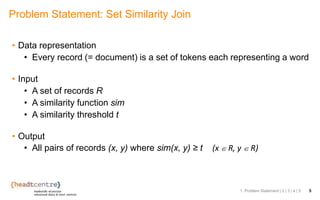
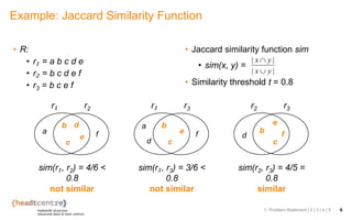
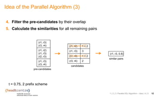
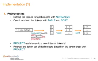
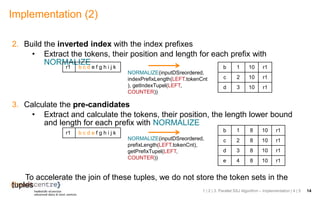
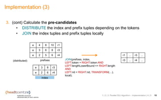
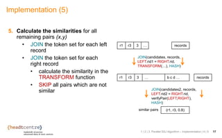
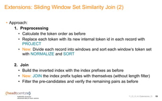
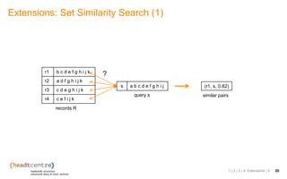
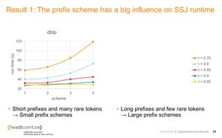
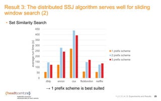
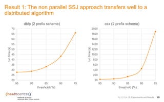
Innovation and Reinvention
Driving Transformation
OCTOBER 9, 2018
2018 HPCC Systems® Community Day
Fabian Fier
Set Similarity Join and Search
with different Prefix Schemes
Background
Motivation & Agenda | 1 | 2 | 3 | 4 | 5 3
• Many applications need to identify similar
pairs of documents:
• Plagiarism detection
• Community mining in social networks
• Near-duplicate web page detection
• Document clustering
• ...
• Problem: Large amounts of data
• Solution: Parallel set similarity join
algorithms (SSJ)
Motivation
Motivation & Agenda | 1 | 2 | 3 | 4 | 5 4
Agenda
1. Problem Statement
2. Filter-Verification
Framework
3. Parallel SSJ Algorithm
a. Idea
b. Implementation
4. Extensions
a. Sliding-Window SSJ
b. Set Similarity Search
5. Experiments and Results
• Data representation
• Every record (= document) is a set of tokens each representing a word
• Input
• A set of records R
• A similarity function sim
• A similarity threshold t
• Output
• All pairs of records (x, y) where sim(x, y) ≥ t (x ∈ R, y ∈ R)
Problem Statement: Set Similarity Join
1. Problem Statement | 2 | 3 | 4 | 5 5
Example: Jaccard Similarity Function
• R:
• r₁ = a b c d e
• r₂ = b c d e f
• r3 = b c e f
• Jaccard similarity function sim
• sim(x, y) =
• Similarity threshold t = 0.8
1. Problem Statement | 2 | 3 | 4 | 5 6
||
||
yx
yx


a
db
e
c
f
r₁ r2
a
d
b
e
c
f
r₁ r3
d
b
e
c
f
r2 r3
sim(r₁, r2) = 4/6 <
0.8
not similar
sim(r₁, r3) = 3/6 <
0.8
not similar
sim(r2, r3) = 4/5 =
0.8
similar
• Naive Solution
• Calculating similarity value for each pair
→ Too expensive
• Better
• Filter-verification framework
• Filter step: Use filter to prune all pairs that cannot be similar
• Verification step: Compute the similarity value for the remaining
pairs
How to calculate these pairs efficiently?
1 | 2. Filter-Verification Framework | 3 | 4 | 5 7
• Prefix filtering
• (x,y) can only be similar if their prefixes share at least one token
• Length filtering
• Only documents with a similar length can be similar
Common Filter Techniques
1 | 2. Filter-Verification Framework | 3 | 4 | 5 8
e f h
a b h k
a b c d
he f
h
prefixes
→ Our goal: Implement this approach as a parallel algorithm
• Experiments with different prefix schemes
• Extend it to a set similarity search and a sliding window SSJ algorithm
General Approach
1 | 2. Filter-Verification Framework | 3 | 4 | 5 9
r1 b c d e f g h i j k
r2 a d f g h i j k
r3 c d e g h i j k
r4 c e f i j k
1. Build index on prefixes of R
records R, t = 0.75
a r2
b r1
c r1, r3, r4
d r2, r3
index
2. Probe (filter) for each record
example: r1
list for each
prefix token
b r1
c r1, r3, r4
d r2, r3
candidates
(r1, r2)
(r1, r3)
(r1, r4)
3. Verification
(r1, r3, 0.8)
prefix scheme +1
→ prefix size +1
→ needed overlap +1
a r2
b r1
c r1, r3, r4
d r2, r3, r1
e r3, r4
f r2
b r1
c r1, r3, r4
d r2, r3, r1
e r3, r4
similar pairs
1. Preprocessing: order token sets by global token frequency
2. Build the inverted index on the prefixes
Idea of the Parallel Algorithm (1)
1 | 2 | 3. Parallel SSJ Algorithm – Idea | 4 | 5 10
r1 b c d e f g h i j k
r2 a d f g h i j k
r3 c d e g h i j k
r4 c e f i j k
records R
a r2
b r1
c r1
r3,
r4
d r1,
r2,
r3
e r3,
r4
f r2
t = 0.75, 2 prefix scheme index
Idea of the Parallel Algorithm (2)
3. Calculate the pre-candidates
1 | 2 | 3. Parallel SSJ Algorithm – Idea | 4 | 5 11
t = 0.75, 2 prefix scheme
r1 b c d e f g h i j k
r2 a d f g h i j k
r3 c d e g h i j k
r4 c e f i j k
records R
a r2
b r1
c r1,
r3,
r4
d r1,
r2,
r3
e r1,
r3,
r4
f r2,
r4
g r2,
r3
prefixes
a r2
b r1
c r1
r3,
r4
d r1,
r2,
r3
e r3,
r4
f r2
index
⋈ 𝑓𝑖𝑙𝑡𝑒𝑟
𝑟𝑖𝑑 𝑙 < 𝑟𝑖𝑑 𝑟
(r1, r3)
(r1, r4)
(r3, r4)
(r1, r2)
(r1, r3)
(r2, r3)
(r1, r3)
(r1, r4)
(r3, r4)
length
length
pre-candidates
4. Filter the pre-candidates by their overlap
5. Calculate the similarities for all remaining pairs
Idea of the Parallel Algorithm (3)
1 | 2 | 3. Parallel SSJ Algorithm – Idea | 4 | 5 12
t = 0.75, 2 prefix scheme
(r1, r3)
(r3, r4)
(r1, r2)
(r1, r3)
(r2, r3)
(r1, r3)
(r3, r4)
pre-candidates
(r1, r2) 1 < 2
(r1, r3) 3
(r2, r3) 1 < 2
(r3, r4) 2
candidates
(r1, r3, 0.8)
similar pairs
1. Preprocessing
• Extract the tokens for each record with NORMALIZE
• Count and sort the tokens with TABLE and SORT
• PROJECT each token to a new internal token id
• Reorder the token set of each record based on the token order with
PROJECT
Implementation (1)
1 | 2 | 3. Parallel SSJ Algorithm – Implementation | 4 | 5 13
r1 b k c d e f i g h j
NORMALIZE(inputDS,
LEFT.tokenCnt,
extractToken(LEFT,
COUNTER))
b
k
… TABLE
b 1
k 4
… SORT
a 1
…
k 4
2. Build the inverted index with the index prefixes
• Extract the tokens, their position and length for each prefix with
NORMALIZE
3. Calculate the pre-candidates
• Extract and calculate the tokens, their position, the length lower bound
and length for each prefix with NORMALIZE
To accelerate the join of these tuples, we do not store the token sets in the
tuples
Implementation (2)
1 | 2 | 3. Parallel SSJ Algorithm – Implementation | 4 | 5 14
r1 b c d e f g h i j k b 1 10 r1
c 2 10 r1
d 3 10 r1
NORMALIZE(inputDSreordered,
indexPrefixLength(LEFT.tokenCnt
), getIndexTupel(LEFT,
COUNTER))
r1 b c d e f g h i j k b 1 8 10 r1
c 2 8 10 r1
d 3 8 10 r1
e 4 8 10 r1
NORMALIZE(inputDSreordered,
prefixLength(LEFT.tokenCnt),
getPrefixTupel(LEFT,
COUNTER))
3. (cont) Calculate the pre-candidates
• DISTRIBUTE the index and prefix tuples depending on the tokens
• JOIN the index tuples and prefix tuples locally
Implementation (3)
1 | 2 | 3. Parallel SSJ Algorithm – Implementation | 4 | 5 15
e 3 8 r3
e 2 6 r4
e 4 8 10 r1
e 3 6 8 r3
e 2 5 6 r4
(distributed) prefixes
index
r1 … r3 …
r3 … r4 …JOIN(prefixes, index,
LEFT.token = RIGHT.token AND
LEFT.lengthLowerBound <= RIGHT.length
AND
LEFT.rid < RIGHT.rid, TRANSFORM(…),
local);
4. Filter the pre-candidates
• Count the overlap of each pair with DISTRIBUTE, SORT and ROLLUP
• SKIP all pairs which do not pass the position filter
• Check the overlap of each pair with PROJECT and SKIP if necessary
Implementation (4)
1 | 2 | 3. Parallel SSJ Algorithm – Implementation | 4 | 5 16
ROLLUP(tupelDS,
LEFT.rid1 = RIGHT.rid1 and
LEFT.rid2 = RIGHT.rid2,
countOverlap(LEFT,RIGHT),
local)
r1 r3 3 …
(distributed
and sorted
depending
on rids)
r1 … r3 …
r1 … r3 …
r1 … r3 …
r1 … r2 …
ROLLUP(…)
r1 r2 1 …
r1 r3 3 …
PROJECT
PROJECT
Implementation (5)
5. Calculate the similarities for all
remaining pairs (x,y)
• JOIN the token set for each left
record
• JOIN the token set for each
right record
• calculate the similarity in the
TRANSFORM function
• SKIP all pairs which are not
similar
1 | 2 | 3. Parallel SSJ Algorithm – Implementation | 4 | 5 17
(r1, r3, 0.8)
JOIN(candidates, records,
LEFT.rid1 = RIGHT.rid,
TRANSFORM(…), HASH)
similar pairs
r1 r3 3 … b c d …
recordsr1 r3 3 …
JOIN(candidates2, records,
LEFT.rid2 = RIGHT.rid,
verifyPair(LEFT,RIGHT),
HASH)
records
• Divide each record into windows of size w
• Search all window pairs (xi,yj) with sim(xi,yj) ≥ t (x,y in R, |xi|=|yj|=w)
Extensions: Sliding Window Set Similarity Join (1)
1 | 2 | 3 | 4. Extensions | 5 18
x
x1
x2
x3
x4
x5
w
• Approach:
1. Preprocessing
• Calculate the token order as before
• Replace each token with its new internal token id in each record with
PROJECT
• New: Divide each record into windows and sort each window‘s token set
with NORMALIZE and SORT
2. Join
• Build the inverted index with the index prefixes as before
• New: JOIN the index prefix tuples with themselves (without length filter)
• Filter the pre-candidates and verify the remaining pairs as before
Extensions: Sliding Window Set Similarity Join (2)
1 | 2 | 3 | 4. Extensions | 5 19
Extensions: Set Similarity Search (1)
1 | 2 | 3 | 4. Extensions | 5 20
r1 b c d e f g h i j k
r2 a d f g h i j k
r3 c d e g h i j k
r4 c e f i j k
records R
query s
s a b c d e f g h i j (r1, s, 0.82)
similar pairs
?
• Approach:
1. Preparation with THOR
• Calculate the token order as before
• New: BUILD two payload INDEXes for them
2. New: Searching with ROXIE
• Preprocess the query record
• Use an INDEX JOIN with the token order and SORT to reorder the
tokens
• Calculate the pre-candidates and candidates as before and verify them
• Use an INDEX JOIN with the index to find the pre-candidates
Extensions: Set Similarity Search (2)
1 | 2 | 3 | 4. Extensions | 5 21
token id new token idtoken order
key payload
token id, length rid, pos, token setindex
key payload
• Datasets
• flickrlondon, dblp, enron, netflix, csx
• patent data 2005 and 2010
• Cluster configuration
• 6 Thor nodes
• 3 Thor slaves per node
Experiments and Results
1 | 2 | 3 | 4 | 5. Experiments and Results 22
dataset size
record
count
average record
length
flickrlondon 253 MB 1680490 9.8
dblp 685 MB 1268017 36.2
enron 1.0 GB 517431 133.6
netflix 1.1 GB 480189 209.3
csx 3.5 GB 1385532 148.9
2005 9.5 GB 157829 7248.7 (1814.7*)
2010 16.5 GB 244597 8175.3 (1999,9*)
* without stopwords
Result 1: The prefix scheme has a big influence on SSJ runtime
• Short prefixes and many rare tokens
→ Small prefix schemes
• Long prefixes and few rare tokens
→ Large prefix schemes
1 | 2 | 3 | 4 | 5. Experiments and Results 23
20
40
60
80
100
120
1 2 3 4
runtime(s)
scheme
dblp
0
1000
2000
3000
4000
5000
6000
1 2 3 4
runtime(s)
scheme
netflix
t = 0.75
t = 0.8
t = 0.85
t = 0.9
t = 0.95
• Sliding Window SSJ
Result 2: The distributed SSJ algorithm serves well for sliding
window join
1 | 2 | 3 | 4 | 5. Experiments and Results 24
Disk full
0
1000
2000
3000
4000
5000
6000
7000
8000
9000
1 2 3 4
runtime(s)
scheme
Patent 2005 (without stopwords), w = 100
t = 0.75
t = 0.8
t = 0.85
t = 0.9
t = 0.95
→ Same prefix scheme behavior as before
0
500
1000
1500
2000
2500
3000
7580859095
runtime(s)
threshold (%)
Patent 2005 (without stopwords), 3 prefix
scheme
w = 50
w = 100
→ Smaller window size needs more time
• Set Similarity Search
Result 3: The distributed SSJ algorithm serves well for sliding
window search (2)
1 | 2 | 3 | 4 | 5. Experiments and Results 25
0
50
100
150
200
250
300
350
400
450
dblp enron csx flicklondon netflix
averageruntime(s)
1 prefix scheme
2 prefix scheme
3 prefix scheme
→ 1 prefix scheme is best suited
• Questions?
Thank you!
26
• Prefix filtering
• (x,y) can only be similar if their prefixes share at least one token
• Length filtering
• Only documents with a similar length can be similar
• Position filtering
• (x,y) can only be similar if the postfix is long enough
Common Filter Techniques
1 | 2. Filter-Verification Framework | 3 | 4 | 5 27
w
w
i
j
x
y
|x| - i
|y| - j
overlapw + 1 + min(|x|-i, |y|-j) ≥
𝑡
1+𝑡
(|x|+|y|)
?
e f h
a b h k
a b c d
he f
h
prefixes
1. Preprocessing
• Read the input record set R
• Count token appearances and calculate the token ordering T
• Reorder the token set of each record based on the token ordering T
Idea of the Distributed Algorithm (1)
1 | 2 | 3. Distributed SSJ Algorithm – Idea | 4 | 5 28
r1 b k c d e f i g h j
r2 a d f k g h i j
r3 c k d e j g h i
r4 c e j f i k
a 1
b 1
c 3
d 3
…
k 4records R (unordered)
token order T
r1 b c d e f g h i j k
r2 a d f g h i j k
r3 c d e g h i j k
r4 c e f i j k
records R (ordered)
Result 1: The non parallel SSJ approach transfers well to a
distributed algorithm
20
25
30
35
40
45
50
55
60
65
70
7580859095
runtime(s)
threshold (%)
dblp (2 prefix scheme)
1 | 2 | 3 | 4 | 5. Experiments and Results 29
20
220
420
620
820
1020
1220
1420
1620
1820
2020
7580859095
runtime(s) threshold (%)
csx (2 prefix scheme)

Optimizing Set-Similarity Join and Search with Different Prefix Schemes

  • 2.
    Innovation and Reinvention DrivingTransformation OCTOBER 9, 2018 2018 HPCC Systems® Community Day Fabian Fier Set Similarity Join and Search with different Prefix Schemes
  • 3.
    Background Motivation & Agenda| 1 | 2 | 3 | 4 | 5 3
  • 4.
    • Many applicationsneed to identify similar pairs of documents: • Plagiarism detection • Community mining in social networks • Near-duplicate web page detection • Document clustering • ... • Problem: Large amounts of data • Solution: Parallel set similarity join algorithms (SSJ) Motivation Motivation & Agenda | 1 | 2 | 3 | 4 | 5 4 Agenda 1. Problem Statement 2. Filter-Verification Framework 3. Parallel SSJ Algorithm a. Idea b. Implementation 4. Extensions a. Sliding-Window SSJ b. Set Similarity Search 5. Experiments and Results
  • 5.
    • Data representation •Every record (= document) is a set of tokens each representing a word • Input • A set of records R • A similarity function sim • A similarity threshold t • Output • All pairs of records (x, y) where sim(x, y) ≥ t (x ∈ R, y ∈ R) Problem Statement: Set Similarity Join 1. Problem Statement | 2 | 3 | 4 | 5 5
  • 6.
    Example: Jaccard SimilarityFunction • R: • r₁ = a b c d e • r₂ = b c d e f • r3 = b c e f • Jaccard similarity function sim • sim(x, y) = • Similarity threshold t = 0.8 1. Problem Statement | 2 | 3 | 4 | 5 6 || || yx yx   a db e c f r₁ r2 a d b e c f r₁ r3 d b e c f r2 r3 sim(r₁, r2) = 4/6 < 0.8 not similar sim(r₁, r3) = 3/6 < 0.8 not similar sim(r2, r3) = 4/5 = 0.8 similar
  • 7.
    • Naive Solution •Calculating similarity value for each pair → Too expensive • Better • Filter-verification framework • Filter step: Use filter to prune all pairs that cannot be similar • Verification step: Compute the similarity value for the remaining pairs How to calculate these pairs efficiently? 1 | 2. Filter-Verification Framework | 3 | 4 | 5 7
  • 8.
    • Prefix filtering •(x,y) can only be similar if their prefixes share at least one token • Length filtering • Only documents with a similar length can be similar Common Filter Techniques 1 | 2. Filter-Verification Framework | 3 | 4 | 5 8 e f h a b h k a b c d he f h prefixes
  • 9.
    → Our goal:Implement this approach as a parallel algorithm • Experiments with different prefix schemes • Extend it to a set similarity search and a sliding window SSJ algorithm General Approach 1 | 2. Filter-Verification Framework | 3 | 4 | 5 9 r1 b c d e f g h i j k r2 a d f g h i j k r3 c d e g h i j k r4 c e f i j k 1. Build index on prefixes of R records R, t = 0.75 a r2 b r1 c r1, r3, r4 d r2, r3 index 2. Probe (filter) for each record example: r1 list for each prefix token b r1 c r1, r3, r4 d r2, r3 candidates (r1, r2) (r1, r3) (r1, r4) 3. Verification (r1, r3, 0.8) prefix scheme +1 → prefix size +1 → needed overlap +1 a r2 b r1 c r1, r3, r4 d r2, r3, r1 e r3, r4 f r2 b r1 c r1, r3, r4 d r2, r3, r1 e r3, r4 similar pairs
  • 10.
    1. Preprocessing: ordertoken sets by global token frequency 2. Build the inverted index on the prefixes Idea of the Parallel Algorithm (1) 1 | 2 | 3. Parallel SSJ Algorithm – Idea | 4 | 5 10 r1 b c d e f g h i j k r2 a d f g h i j k r3 c d e g h i j k r4 c e f i j k records R a r2 b r1 c r1 r3, r4 d r1, r2, r3 e r3, r4 f r2 t = 0.75, 2 prefix scheme index
  • 11.
    Idea of theParallel Algorithm (2) 3. Calculate the pre-candidates 1 | 2 | 3. Parallel SSJ Algorithm – Idea | 4 | 5 11 t = 0.75, 2 prefix scheme r1 b c d e f g h i j k r2 a d f g h i j k r3 c d e g h i j k r4 c e f i j k records R a r2 b r1 c r1, r3, r4 d r1, r2, r3 e r1, r3, r4 f r2, r4 g r2, r3 prefixes a r2 b r1 c r1 r3, r4 d r1, r2, r3 e r3, r4 f r2 index ⋈ 𝑓𝑖𝑙𝑡𝑒𝑟 𝑟𝑖𝑑 𝑙 < 𝑟𝑖𝑑 𝑟 (r1, r3) (r1, r4) (r3, r4) (r1, r2) (r1, r3) (r2, r3) (r1, r3) (r1, r4) (r3, r4) length length pre-candidates
  • 12.
    4. Filter thepre-candidates by their overlap 5. Calculate the similarities for all remaining pairs Idea of the Parallel Algorithm (3) 1 | 2 | 3. Parallel SSJ Algorithm – Idea | 4 | 5 12 t = 0.75, 2 prefix scheme (r1, r3) (r3, r4) (r1, r2) (r1, r3) (r2, r3) (r1, r3) (r3, r4) pre-candidates (r1, r2) 1 < 2 (r1, r3) 3 (r2, r3) 1 < 2 (r3, r4) 2 candidates (r1, r3, 0.8) similar pairs
  • 13.
    1. Preprocessing • Extractthe tokens for each record with NORMALIZE • Count and sort the tokens with TABLE and SORT • PROJECT each token to a new internal token id • Reorder the token set of each record based on the token order with PROJECT Implementation (1) 1 | 2 | 3. Parallel SSJ Algorithm – Implementation | 4 | 5 13 r1 b k c d e f i g h j NORMALIZE(inputDS, LEFT.tokenCnt, extractToken(LEFT, COUNTER)) b k … TABLE b 1 k 4 … SORT a 1 … k 4
  • 14.
    2. Build theinverted index with the index prefixes • Extract the tokens, their position and length for each prefix with NORMALIZE 3. Calculate the pre-candidates • Extract and calculate the tokens, their position, the length lower bound and length for each prefix with NORMALIZE To accelerate the join of these tuples, we do not store the token sets in the tuples Implementation (2) 1 | 2 | 3. Parallel SSJ Algorithm – Implementation | 4 | 5 14 r1 b c d e f g h i j k b 1 10 r1 c 2 10 r1 d 3 10 r1 NORMALIZE(inputDSreordered, indexPrefixLength(LEFT.tokenCnt ), getIndexTupel(LEFT, COUNTER)) r1 b c d e f g h i j k b 1 8 10 r1 c 2 8 10 r1 d 3 8 10 r1 e 4 8 10 r1 NORMALIZE(inputDSreordered, prefixLength(LEFT.tokenCnt), getPrefixTupel(LEFT, COUNTER))
  • 15.
    3. (cont) Calculatethe pre-candidates • DISTRIBUTE the index and prefix tuples depending on the tokens • JOIN the index tuples and prefix tuples locally Implementation (3) 1 | 2 | 3. Parallel SSJ Algorithm – Implementation | 4 | 5 15 e 3 8 r3 e 2 6 r4 e 4 8 10 r1 e 3 6 8 r3 e 2 5 6 r4 (distributed) prefixes index r1 … r3 … r3 … r4 …JOIN(prefixes, index, LEFT.token = RIGHT.token AND LEFT.lengthLowerBound <= RIGHT.length AND LEFT.rid < RIGHT.rid, TRANSFORM(…), local);
  • 16.
    4. Filter thepre-candidates • Count the overlap of each pair with DISTRIBUTE, SORT and ROLLUP • SKIP all pairs which do not pass the position filter • Check the overlap of each pair with PROJECT and SKIP if necessary Implementation (4) 1 | 2 | 3. Parallel SSJ Algorithm – Implementation | 4 | 5 16 ROLLUP(tupelDS, LEFT.rid1 = RIGHT.rid1 and LEFT.rid2 = RIGHT.rid2, countOverlap(LEFT,RIGHT), local) r1 r3 3 … (distributed and sorted depending on rids) r1 … r3 … r1 … r3 … r1 … r3 … r1 … r2 … ROLLUP(…) r1 r2 1 … r1 r3 3 … PROJECT PROJECT
  • 17.
    Implementation (5) 5. Calculatethe similarities for all remaining pairs (x,y) • JOIN the token set for each left record • JOIN the token set for each right record • calculate the similarity in the TRANSFORM function • SKIP all pairs which are not similar 1 | 2 | 3. Parallel SSJ Algorithm – Implementation | 4 | 5 17 (r1, r3, 0.8) JOIN(candidates, records, LEFT.rid1 = RIGHT.rid, TRANSFORM(…), HASH) similar pairs r1 r3 3 … b c d … recordsr1 r3 3 … JOIN(candidates2, records, LEFT.rid2 = RIGHT.rid, verifyPair(LEFT,RIGHT), HASH) records
  • 18.
    • Divide eachrecord into windows of size w • Search all window pairs (xi,yj) with sim(xi,yj) ≥ t (x,y in R, |xi|=|yj|=w) Extensions: Sliding Window Set Similarity Join (1) 1 | 2 | 3 | 4. Extensions | 5 18 x x1 x2 x3 x4 x5 w
  • 19.
    • Approach: 1. Preprocessing •Calculate the token order as before • Replace each token with its new internal token id in each record with PROJECT • New: Divide each record into windows and sort each window‘s token set with NORMALIZE and SORT 2. Join • Build the inverted index with the index prefixes as before • New: JOIN the index prefix tuples with themselves (without length filter) • Filter the pre-candidates and verify the remaining pairs as before Extensions: Sliding Window Set Similarity Join (2) 1 | 2 | 3 | 4. Extensions | 5 19
  • 20.
    Extensions: Set SimilaritySearch (1) 1 | 2 | 3 | 4. Extensions | 5 20 r1 b c d e f g h i j k r2 a d f g h i j k r3 c d e g h i j k r4 c e f i j k records R query s s a b c d e f g h i j (r1, s, 0.82) similar pairs ?
  • 21.
    • Approach: 1. Preparationwith THOR • Calculate the token order as before • New: BUILD two payload INDEXes for them 2. New: Searching with ROXIE • Preprocess the query record • Use an INDEX JOIN with the token order and SORT to reorder the tokens • Calculate the pre-candidates and candidates as before and verify them • Use an INDEX JOIN with the index to find the pre-candidates Extensions: Set Similarity Search (2) 1 | 2 | 3 | 4. Extensions | 5 21 token id new token idtoken order key payload token id, length rid, pos, token setindex key payload
  • 22.
    • Datasets • flickrlondon,dblp, enron, netflix, csx • patent data 2005 and 2010 • Cluster configuration • 6 Thor nodes • 3 Thor slaves per node Experiments and Results 1 | 2 | 3 | 4 | 5. Experiments and Results 22 dataset size record count average record length flickrlondon 253 MB 1680490 9.8 dblp 685 MB 1268017 36.2 enron 1.0 GB 517431 133.6 netflix 1.1 GB 480189 209.3 csx 3.5 GB 1385532 148.9 2005 9.5 GB 157829 7248.7 (1814.7*) 2010 16.5 GB 244597 8175.3 (1999,9*) * without stopwords
  • 23.
    Result 1: Theprefix scheme has a big influence on SSJ runtime • Short prefixes and many rare tokens → Small prefix schemes • Long prefixes and few rare tokens → Large prefix schemes 1 | 2 | 3 | 4 | 5. Experiments and Results 23 20 40 60 80 100 120 1 2 3 4 runtime(s) scheme dblp 0 1000 2000 3000 4000 5000 6000 1 2 3 4 runtime(s) scheme netflix t = 0.75 t = 0.8 t = 0.85 t = 0.9 t = 0.95
  • 24.
    • Sliding WindowSSJ Result 2: The distributed SSJ algorithm serves well for sliding window join 1 | 2 | 3 | 4 | 5. Experiments and Results 24 Disk full 0 1000 2000 3000 4000 5000 6000 7000 8000 9000 1 2 3 4 runtime(s) scheme Patent 2005 (without stopwords), w = 100 t = 0.75 t = 0.8 t = 0.85 t = 0.9 t = 0.95 → Same prefix scheme behavior as before 0 500 1000 1500 2000 2500 3000 7580859095 runtime(s) threshold (%) Patent 2005 (without stopwords), 3 prefix scheme w = 50 w = 100 → Smaller window size needs more time
  • 25.
    • Set SimilaritySearch Result 3: The distributed SSJ algorithm serves well for sliding window search (2) 1 | 2 | 3 | 4 | 5. Experiments and Results 25 0 50 100 150 200 250 300 350 400 450 dblp enron csx flicklondon netflix averageruntime(s) 1 prefix scheme 2 prefix scheme 3 prefix scheme → 1 prefix scheme is best suited
  • 26.
  • 27.
    • Prefix filtering •(x,y) can only be similar if their prefixes share at least one token • Length filtering • Only documents with a similar length can be similar • Position filtering • (x,y) can only be similar if the postfix is long enough Common Filter Techniques 1 | 2. Filter-Verification Framework | 3 | 4 | 5 27 w w i j x y |x| - i |y| - j overlapw + 1 + min(|x|-i, |y|-j) ≥ 𝑡 1+𝑡 (|x|+|y|) ? e f h a b h k a b c d he f h prefixes
  • 28.
    1. Preprocessing • Readthe input record set R • Count token appearances and calculate the token ordering T • Reorder the token set of each record based on the token ordering T Idea of the Distributed Algorithm (1) 1 | 2 | 3. Distributed SSJ Algorithm – Idea | 4 | 5 28 r1 b k c d e f i g h j r2 a d f k g h i j r3 c k d e j g h i r4 c e j f i k a 1 b 1 c 3 d 3 … k 4records R (unordered) token order T r1 b c d e f g h i j k r2 a d f g h i j k r3 c d e g h i j k r4 c e f i j k records R (ordered)
  • 29.
    Result 1: Thenon parallel SSJ approach transfers well to a distributed algorithm 20 25 30 35 40 45 50 55 60 65 70 7580859095 runtime(s) threshold (%) dblp (2 prefix scheme) 1 | 2 | 3 | 4 | 5. Experiments and Results 29 20 220 420 620 820 1020 1220 1420 1620 1820 2020 7580859095 runtime(s) threshold (%) csx (2 prefix scheme)

Editor's Notes

  • #6 hier nur Self-Join betrachtet
  • #7 @Fabian: ggf. nur eines der Bilder nehmen (wegen Zeit)
  • #8 „Filter-verification framework“ ist ein verbreiteter Ansatz; aber natürlich nicht die einzige Lösung
  • #9 - WICHTIG: selbe Tokenorder (bei prefix und position) -> sonst klappt es nicht! - optimal: seltene Token vorne (weniger Überschneidungen -> weniger Kandidaten)
  • #10 Allg. Vorgehen mit Prefix Filtering „candidates“ können zusätzlich mit anderen Filtern weiter reduziert werden (hier der Einfachheit halber nicht gezeigt) Idee für Präfixvergrößerung aus: „Can We Beat the Prefix Filtering? An Adaptive Framework for Similarity Join and Search“ von J. Wang, G. Li and J. Feng
  • #12 Join-Bedingung: Präfix- und Längenfilter sowie Self-Join Bedingung (Rid-Vergleich abhängig von Länge, um Dopplungen (x,y) und (y,x) sowie Identitäten (x,x) zu vermeiden) Self-Join-Bedingung lässt sich im Bsp. einfach als (rid aus prefix) < (rid aus index) formulieren, da die Records im Bsp. nach Längen sortiert sind Diese Vereinfachung wird im Folgenden stets benutzt
  • #14 Zu den letzten Punkte keine Bilder (da uninteressant): „PROJECT each token to a new internal token id“: a -> 1, b -> 2 etc. (ähnlich einer Map Funktion) “Reorder the token set of each record based on the token order with PROJECT”: b k c d e f i g h j -> b c d e f g h i j k bzw. die neuen Ids (in jeder Tokenmenge werden die Tokens mit den internen Ids ersetzt und sortiert; dafür wird ein Project verwendet, indem wiederum Funktionen zum Tauschen und Sortieren aufgerufen werden)
  • #15 wie im Bsp. zuvor l=2 als Schema
  • #16 wie im Bsp. zuvor l=2 als Schema Join-Bedingung wurde etwas vereinfacht (nur Rid-Vergleich wie vorne) nicht alle ECL Join-Optionen sind angegeben (noch unordered, inner und limit(0))
  • #17 wie im Bsp. zuvor l=2 als Schema; Code etwas vereinfacht dargestellt: es wir zunächst nach rids verteilt mit DISTRIBUTE und nach rids und positionen sortiert mit SORT (wichtig für position filtering) ROLLUP gruppiert die Tupel nach den rid-paaren, zählt den overlap pro Paar und testet dabei den pos. Filter wenn ein Paar nur einmal vorkommt, wird es bei ROLLUP nicht bearbeitet, sondern einfach nur ausgegeben deshalb wird beim Join davor schon bei jedem Tupel ein overlap von 1 mitgespeichert im abschließenden Project wird der overlap kontrolliert und, falls das Schema l=1 ist, für alle Paare mit overlap 1 der pos. Filter noch angewandt
  • #19 - anders als beim SSJ: statt ganze Records werden Teile der Records verglichen - Wir nutzen immer 50% Überlappung der Windows (und ggf. letztes Window mit mehr Überlappung, wenn es nicht aufgeht -> siehe y)
  • #20 1. Preprocessing: nur replace und nicht reorder (wie zuvor) sortiert wird erst in den einzelnen Windows (da wir vorm Zerteilen nicht die Reihenfolge ändern dürfen) wir haben die Window-Size als Parameter und 50% Überlappung der Windows 2. Join Index aus Indexpräfixen wie zuvor Dann direkt einen Self-Join des Indexes (Berechnung der Präfixe und Join damit ist unnötig, da durch die einheitliche Länge die Indexpräfixe auf beiden Seiten des Joins ausreichen) alles zum Thema Länge kann weggelassen werden (also keine length oder lengthlowerbound in den Records, kein Längenfilter im Join)
  • #21 Anders als bei SSJ: statt Records mit Records zu joinen gibt es nur ein Record (die Query) als Join-Partner
  • #22 Preparation: - Neu: Tokenmengen werden mit im Index gespeichert (da nur eine Query mit dem Index gejoint wird, ist dieser zusätzliche Platz im Index / beim Join weniger gravierend und der Join mit den originalen Records am Ende kann weggelassen werden; zudem müssen so die originalen Records in Roxie nicht eingelesen werden)
  • #23 restliche Zahlen (Tokenhäufigkeiten, Ergebnisanzahl, etc.) in messwerte.ods
  • #24 Laufzeiten bei verschiedenen Schwellwerten Dblp als Beispiel für kurze Präfixe + seltene Token -> bei allen getesteten Schwellwerten ist ein kleines Schema (1) besser Netflix als Beispiel für länge Präfixe + wenige seltene Token -> bei allen getesteten Schwellwerten ist ein größeres Schema (meist 3) besser Mit kleineren Schwellwerten steigt das optimale Schema (hier in den Bildern nicht zu sehen, aber indirekt enthalten: kleinere t -> längere Präfixe -> Schema muss größer werden)
  • #25 Beispiele von Datensätzen MIT Stopword Removal, da ohne dies die Messungen oft wegen „System Error: Disk full“ abgebrochen sind bei mit Stopwords: nur wenige Messwerte zum Vergleichen Preprocessing ist hier nicht dargestellt, nur der Join (restl. Werte in messwerte.ods) Links: selbes Verhalten wie zuvor: Mit kleineren Schwellwerten steigt das optimale Schema (optimal waren in den Tests meist 2 oder 3 bei w=100 und w=50 und stopword removal) Recht: Vergleich von window sizes (kleinere window size -> mehr Windows -> längere Laufzeiten) Bei w = 100 ca. 1 Mio windows, bei w = 50 ca. 2 Mio windows
  • #26 Beispiele von Datensätzen MIT Stopword Removal, da ohne dies die Messungen oft wegen „System Error: Disk full“ abgebrochen sind Preprocessing ist hier nicht drin, nur Search (restl. Werte in messwerte.ods) Im Bild: Mittelwert der Laufzeiten der Suche auf ROXIE pro Balken: Mittelwert aus 6 Messungen (3 verschiedene Queries je 2 mal getestet; nie zwei mal hintereinander der selbe Datensatz wegen Caching) Man sieht das 1 als Schema hier am schnellsten ist (vermutlich da der Index kleiner ist und es bei einer Query auch nur wenige Kandidaten gibt, also die Verifikation schnell ist -> Präfixvergrößerung ist somit hier sinnlos)
  • #28 - WICHTIG: selbe Tokenorder (bei prefix und position) -> sonst klappt es nicht! - optimal: seltene Token vorne (weniger Überschneidungen -> weniger Kandidaten)
  • #29 @Fabian: falls es zu lang wird, kann diese Folie auch nur kurz angeschnitten werden (da relativ uninteressant)
  • #30 Die Folie könnte man auch weglassen und nur sagen: „Wie haben gezeigt, dass sich der lokale Algorithmus in einer verteilten, parallelen Algorithmus überführen lässt. Bla bla bla. Und nun Präfixschemaerkenntnisse und Ergebnis der Erweiterungen…“