Market Policy and Value Chain Analysis

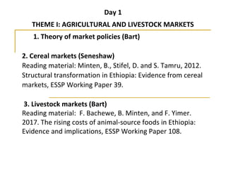
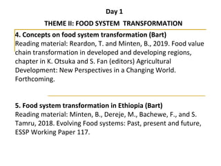
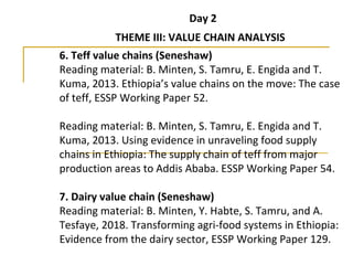
1. Market Policy and Value Chain
Analysis
June 26th
and 27th
2019
EEA
THEME 1: AGRICULTURAL
AND LIVESTOCK MARKETS
EDRI

2. Day 1
THEME I: AGRICULTURAL AND LIVESTOCK MARKETS
1. Theory of market policies (Bart)
2. Cereal markets (Seneshaw)
Reading material: Minten, B., Stifel, D. and S. Tamru, 2012.
Structural transformation in Ethiopia: Evidence from cereal
markets, ESSP Working Paper 39.
3. Livestock markets (Bart)
Reading material: F. Bachewe, B. Minten, and F. Yimer.
2017. The rising costs of animal-source foods in Ethiopia:
Evidence and implications, ESSP Working Paper 108.

3. Day 1
THEME II: FOOD SYSTEM TRANSFORMATION
4. Concepts on food system transformation (Bart)
Reading material: Reardon, T. and Minten, B., 2019. Food value
chain transformation in developed and developing regions,
chapter in K. Otsuka and S. Fan (editors) Agricultural
Development: New Perspectives in a Changing World.
Forthcoming.
5. Food system transformation in Ethiopia (Bart)
Reading material: Minten, B., Dereje, M., Bachewe, F., and S.
Tamru, 2018. Evolving Food systems: Past, present and future,
ESSP Working Paper 117.

4. Day 2
THEME III: VALUE CHAIN ANALYSIS
6. Teff value chains (Seneshaw)
Reading material: B. Minten, S. Tamru, E. Engida and T.
Kuma, 2013. Ethiopia’s value chains on the move: The case
of teff, ESSP Working Paper 52.
Reading material: B. Minten, S. Tamru, E. Engida and T.
Kuma, 2013. Using evidence in unraveling food supply
chains in Ethiopia: The supply chain of teff from major
production areas to Addis Ababa. ESSP Working Paper 54.
7. Dairy value chain (Seneshaw)
Reading material: B. Minten, Y. Habte, S. Tamru, and A.
Tesfaye, 2018. Transforming agri-food systems in Ethiopia:
Evidence from the dairy sector, ESSP Working Paper 129.

5. Market Policy and Value Chain
Analysis
June 26th
and 27th
2019
EEA
THEME 1: AGRICULTURAL
AND LIVESTOCK MARKETS
EDRI

6. Market Policy and Value Chain
Analysis
Session 1:
Theory of Market Policies
EDRI

7. Part 1. Economic equilibrium
Part 2. Spatial equilibrium

8. Part 1. Economic equilibrium:
Objectives
 Define the concepts of economic, partial,
consumer and producer’s equilibrium
 Explain welfare measures
 Explore and practice measuring the efficacy
of policy interventions

9. Outline
 Economic equilibrium
 Welfare measures
 A mathematical formulation

10. Single market/single product
 Consider a market for a product with a “large”
number of producers and a “large” number of
consumers
 We want to know what the price of the
product should be, and how much of the
product should be produced

11. Economic Equilibrium
 Economic equilibrium refers to an
equilibrium in a market that "clears": this is
the case where a market for a product has
attained the price where the
amount supplied of a certain product
equals the quantity demanded

12. Economic Equilibrium, cont.
 Assume market conditions are such that the
price is “very high”
 In this case, producers will be willing to
supply much more than the consumers are
willing to purchase
 An excess of supply results!

13.  Some sellers will be willing to sell cheaper to
find buyers for their excess
 This process repeats until there is no excess
supply left (the market “clears”)
Economic Equilibrium, cont.

14. Economic Equilibrium, cont.
 This price is precisely the equilibrium price!

15. Market Equilibrium
Q supplied
P
Supply
Demand
Q demanded
“Price”
Q

16. Market Equilibrium
Q supplied
P
Supply
Demand
Q demanded
“Price”
Q

17. Market Equilibrium
P
Supply
Demand
Qe
Pe
Q

18. Market Equilibrium
 In an “ideal” economy, this adjustment
process happens instantaneously
 Key assumptions:
 All products are the same
 The equilibrium always exists
 (supply and demand intersect somewhere)

19. Numerical example
Pe = 6 – 0.3Qe (demand curve)
and
Pe = 1 + 0.2Qe (supply curve)
6 – 0.3Qe = 1 + 0.2Qe
5 = 0.5Qe
Qe = 10, Pe = 3

20. Elasticity of demand and supply
 Elasticity is a measure of how demand or
supply responds to a change in price
 Elasticity = percent change in quantity
percent change in price
 Price elasticity of demand is always negative

21. Elasticity of demand and supply
 The steeper a demand or supply curve, the
more inelastic it is
Higher elasticity Lower elasticity

22. Elasticity and Price Stability
P
Q
P
Q

23. Partial Equilibrium
 Partial equilibrium refers to the examination
of one or more closely related markets
 Useful for examining efficiency of policies on the
broad classes of consumers, producers and
government
 Assumes changes in markets examined do not
have large effect on other markets

24. Welfare Measures
 Some consumers are willing to pay more for
a commodity than the prevailing price
 Some producers are willing to accept a price
lower than the prevailing market price

25. Consumers’ Surplus
 The difference between the consumer’s
willingness to pay and the market price is a
measure of benefit to the consumer
 The aggregation of all consumer’s benefits is
a measure of the total benefit to consumers
 Consumer surplus is defined as the area
between the demand curve and the market
price, and between zero and the quantity
consumed

26. Consumers’ Surplus
Demand curve
Quantity consumed
Price
Consumers’ surplus

27. Producers’ Surplus
 The difference between the market price and
the producer’s willingness to accept is a
measure of benefit to the producer
 The aggregation of all producer’s benefits is
a measure of the total benefit to producer
 Producer surplus is defined as the area
between the supply curve and the market
price, and between zero and the quantity
produced

28. Producers’ Surplus
Supply curve
Quantity produced
Price
Producers’ surplus

29. Total welfare
Supply curve
Equilibrium quantity
Equilibrium
Price
Demand curve

30. Market equilibrium, revisited
 Market equilibrium occurs at the
price/quantity combination that maximizes
the sum of consumers’ and producers’
surplus
 This sum is called the quasi-welfare

31. Measuring the Effects of Policy
Intervention
 The benefit (or cost) of imposing a policy
intervention is measured by the difference
between the quasi-welfare with the policy in
place and the quasi-welfare without the
policy (the “baseline”)

32. The Compensation Criterion
 A policy change is socially desirable if as a
result of the change the gainers could
compensate the losers so that no one ended
up worse off
 In the partial equilibrium framework, we will
measure the value of a policy change by the
resulting change in quasi-welfare

33. Part 2. Spatial equilibrium
Objective
 Defining marketing margin
 Discuss the concept of welfare effects
 Explore and discuss mathematical
computation of transport cost

34. Outline
 The marketing margin
 Interregional trade
 Transportation
 A mathematical formulation

35. The Marketing Margin
 The overall difference between the purchase
price of a commodity by consumers and its
sale price by producers
 Can involve costs such as transportation,
broker’s/trader’s fees, value added activities
such as packaging

36. The Marketing Margin
 The marketing margin represents costs of delivering
a product to the consumer, exclusive of production
costs
 The marketing margin drives a wedge between the
price of supply and the price of demand at a given
quantity
 Consider a trader who procures direct from the
supplier and sells directly to the consumer
 This introduces a new supply and demand
curve into the picture

37. The Marketing Margin
SR
SF
DRDF
PR
PF
QE

38. Narrowing the margin
 A key policy objective is often to change the
marketing margin
 Reduce or impose taxes
 Improve transportation infrastructure
 Subsidize inter-seasonal storage

39. Narrowing the margin
S’R
SF
DRD’F
P’R
P’F
Q’E

40. Welfare effects
 If the price elasticity of demand is lower than
the price elasticity of supply, consumers
gain more than producers from a change in
the marketing margin
 if both elasticities are approximately the
same, they share the gain equally
 if the price elasticity of demand is higher
than the price elasticity of demand,
producers gain more than consumers

41. Inter-regional trade
 In countries where supply is spatially distinct
from demand (i.e., rural vs. urban areas),
movement between regions will occur
 Which supply regions ship to which demand
regions depends on many factors
 Transportation costs
 Identifying flows between regions is a key
goal of Spatial Equilibrium Models

42. Two markets, one product, no trade
Market A Market B
PA
PB

43. Two markets, one product, with trade
Market A (exporter) Market B (importer)
P*
PA
PB

44. Gains to Trade
 Quantity available for consumption in
Market A is reduced by Q, and increased in
Market B by Q
 Price increases in the exporting region, and
decreases in the importing region
 Producers gain in the exporting region, and
lose in the importing region

45. Gains to Trade, cont.
 Consumers gain in the importing region,
and lose in the exporting region
 Welfare decreases in the exporting region,
but increases in the importing region

46. 46
DB
PB
PA
P*
SA
Trade sectorCountry A
Exporter
Country B
Importer
DA
EDB
ESA
SB
C
a b
h
g
f
d e
QA0QAD QAS QBS QB0 QBDQAB
Figure: Effect of trade on prices and quantity produced and consumed

47. Condition for Trade
 In the previous example, we have not
considered the transportation costs
 In practice, there will not be trade if the
transportation cost is greater than the
difference between prices in the two
markets

48. Condition for trade
Market A Market B
PA
PB
TC < PB - PA

49. Stability and Trade
 Production less than
QA
 Importer
 Production between
QA and QB
 No trade
 Production greater
than QB
 Exporter
Pw -TC
Pw +TC
QA QB
Pw

50. Transportation
 In reality, there is a cost associated with
transporting goods from one region to
another
 This cost affects:
 Whether or not trade will take place
 The overall benefits to trade

51. Transportation costs
 In general, trade will occur as long as the
transportation cost is less than the difference
between the equilibrium prices (without
trade)
 Transportation costs reduce the overall
gains to trade

52. Modeling Policy Options
 The spatial equilibrium framework is well-
suited to analyze the changes in the market
from changes to the market environment
 It can assess:
 Welfare changes
 Changes in flows of commodities
 Price variability

53. Variable Levies
 A variable levy is a tax (or subsidy) whose
amount is the difference between the world
price of a commodity and a pre-determined
price
 Variable levies can be used to “perfectly”
stabilize price at a given value, or “partially”
stabilize price within a price band

54. Variable Levies
 The amount of a variable levy depends mainly on
two factors:
 The world price of a commodity, and
 The relationship between supply and demand at
the bounds of the price band
 Depending on this relationship, there can be an:
 Export tax
 Export subsidy
 Import tax
 Import subsidy