ANOVA

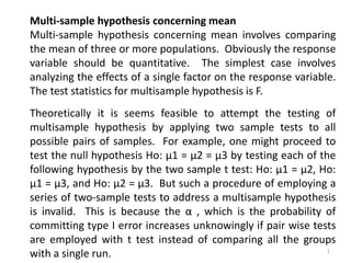
1. Multi-sample hypothesis concerning mean
Multi-sample hypothesis concerning mean involves comparing
the mean of three or more populations. Obviously the response
variable should be quantitative. The simplest case involves
analyzing the effects of a single factor on the response variable.
The test statistics for multisample hypothesis is F.
Theoretically it is seems feasible to attempt the testing of
multisample hypothesis by applying two sample tests to all
possible pairs of samples. For example, one might proceed to
test the null hypothesis Ho: μ1 = μ2 = μ3 by testing each of the
following hypothesis by the two sample t test: Ho: μ1 = μ2, Ho:
μ1 = μ3, and Ho: μ2 = μ3. But such a procedure of employing a
series of two-sample tests to address a multisample hypothesis
is invalid. This is because the α , which is the probability of
committing type I error increases unknowingly if pair wise tests
are employed with t test instead of comparing all the groups
with a single run. 1

2. Illustration of Single factor analysis of variance test
A multisample hypothesis test will be demonstrated with the simplest type
example that involves testing the effect of a single treatment factor on the
response variable involving comparison of three populations.
Consider that the effects of three levels of DAP fertilizer application on the yield
of a given corn variety was evaluated. The three levels of DAP tried were
Level 1 50 kg of DAP per hectare
Level 2 100 kg of DAP per hectare
Level 3 150 kg of DAP per hectare
For the experiment, 15 similar plots of land each measuring (4 m by 5 m) were
prepared. Since the 15 plots were practically similar (e.g. in soil condition,
etc.), they were randomly assigned under the three fertilizer treatments.
Accordingly, 5 plots were assigned under each fertilizer treatment. Then same
variety of corn was sawn in all of the 15 plots. Also all the 15 plots were
managed in a similar manner except that they received different levels of
fertilizer treatment. Upon maturity the corn yield was harvested from all the 15
plots in a single day and the yield from the respective plot was separately
recorded
2

3. The data are shown in the table below. Test if corn yield (quintals/
hectare) differed under the three levels of DAP application? Use 5%
level of significance
Corn yield (Quintals/ hectare) obtained under the three levels of
fertilizer treatments.
Grand sum = ∑∑Xi= 597.5 Grand mean = = 597.5/15 = 39.833
Level of DAP application
50 kg/ hectare 100 kg/ hectare 150 kg/ hectare
33.0 39.0 40.5
34.0 40.5 42.3
35.0 41.2 43.2
35.8 42.1 44.5
37.2 43.5 45.7
= 35.0 = 41.26 = 43.24
= 2.62 = 2.853 = 4.008
∑X1 = 175 ∑X2 = 206.3 ∑X3 = 216.2
1
X 2
X 3
X
3

4. Hypothesis
Ho: The yield of corn is not different under the three
levels of DAP treatments
HA: The yield of corn is different under the three levels of
DAP treatments
4

5. Test statistics
The test statistics for multisample hypothesis test is F. Thus the
procedure is called F test. As in the case of the t test entertained
earlier, F is also computed based on group mean differences, i.e.,
based on the differences of the three group means.
Recall that differences among the three group means is measured by
variance of means ( ) and it is computed as follows.
= SSmeans/df among group (‘a’ is the number of groups tested)
= {(35 – 39.833)2 + (41.26 – 39.833)2 + (43.24 – 39.833)2}/3-1
= 18.5009 Q2/ha
2
X
S
 
1
2
2




a
X
X
S
i
X
5

6. The variance of means expresses differences among the three group
means. Thus, based on the variance of means, a variance known as
variance among group is computed that quantifies the differences in
yield among the three groups of plots. And it is this variance, which is
converted into F statistic.
The variance among group is symbolized as
‘n’ in the above formula is number of replication per group.
Accordingly, S2
among group = 5*18.5009 = 92.5045 Q2/ha
6

7. 7
This implies that the three groups of plots, subjected to
the three different levels of DAP treatments differed by
92.5045 Q2/ha, when their differences is expressed in
terms of variance.
If this variation is considered to be large, then the null
hypothesis that suggests a no yield difference will be
rejected.
To judge if the computed variance among group is
large or not, it is necessary to analyze the sources of
variation in yield among the three groups of plots.

8. 8
The sources of variation in response among the subjects exposed to
different treatments can be described as follows:
i) Treatment caused variation (symbolized as S2
treatment )
One of the reasons why the plots differed in yield is obviously because of
the difference in the treatments. i.e., because the three groups were
treated with three different levels of DAP treatment. This is the explained
portion of the total variability.
ii) Variation in response within respective treatment group (S2
within group)
Not only the three groups of plots differed in yield among one another,
but also the plots within each treatment group differed in yield. For
example as seen from the Table, the variation in yield among the five plots
under the first, second and third levels of DAP treatments are, 2.620,
2.853, and 4.008 Q/ha, respectively. This difference is referred as within
treatment group variability and the reason for this source of variation is
subtle and it is not straight forward to explain. Customarily this source of
variation is referred as unexplained source of variation, since the exact
cause for the variation is not easily explainable.

9. 9
As explained earlier, the 15 plots used for the experiment are similar.
Also the plots under the same fertilizer group are exposed to the
same fertilizer treatment. Then what caused them to differ from one
another?
The exact reason for the within treatment group variation in
response is not clear.
But one thing is evident, that is how ever similar experimental
subjects are, they somehow differ in response and this difference is
therefore the minimum expected variation or unavoidable source of
variation. This source of variation is also commonly referred as error
variance (S2
error) because it occurs as a random error.
In summary the two sources of variation that composed the variance
among group can be expressed as follows.

10. 10
Since the variance within group is the minimum expected
variation, it is used to judge if the variance among group
(S2
among group) that contains the treatment effect is large or not. The
comparison is done as a variance ratio as follows:
when dividing the variance among group with the variance within
group, the treatment effect will be singled out. i.e.,
Accordingly F test is efficient to separately estimate the treatment
effect as long as the denominator variance contains only the
minimum expected variation or random error variance.

11. 11
To complete the computation of Fcal, the variance within group should
be quantified as the average of the three within group variances. If
n1 = n2 =n3,
But the general formula when the replications are unequal is:
(SS1+SS2+SS3)/(df1+df2+df3) = SSwithin group/dfwithin group
dfwithin group can be expressed as (n1 + n2 + n3) -3
Since n1 + n2 + n3 = N (total no. of subjects ) and 3 represents no of
groups (a),
dfwithin group = N – a, i.e., total number of subjects – number of groups

12. 12
In the present example, S2
within group = (2.62+2.853+4.008)/3
= 3.16 Q2/ha
After computing Fcal, the next step is to find out the F
critical value

13. 13
Determining F critical
To determine F critical value for the test, F distribution
is consulted. F is a unit less statistical quantity with a
known distribution.
As explained earlier, F is a variance ratio statistic and F
distribution can be created by repeatedly sampling pair
samples from a given population and dividing the
variance of one of the sample by the variance of the
other sample.
Then plotting the F values against their respective
frequencies gives a positively skewed distribution that
begins at Zero and has a maximum value around one.

14. 14
0
2
4
6
8
10
12
0 1 2 3 4 5 6
Frequency
(%)
F values
F0.05 (2, 12)
3.89
α = 0.05
Figure 10.1 The F distribution constructed based on 2 and
12 degrees of freedom values.
Assume that the treatment effect is zero, i.e., say the fertilizer
differences did not have any effect on yield. This means that the
variance among group would be equal to the variance with in
group. Then the calculated F value becomes 1. This in return
means that a value of F cal 1 represents a perfect agreement or
totally no treatment effect.

15. 15
In practice there is some treatment effect and the
variance among group is expected to be larger than the
variance within group. Hence the calculated F value is
expected to be larger than one. But how large a
calculated value of F indicates a significant treatment
effect? Evidently a calculated F which is large enough to
fall at the extreme right tail indicates a significant
treatment effect. Hence F test is a right tailed test and
the rejection region is an α area at the right tail, in which
α, could be 0.05 or 0.01.
The critical value of F is found in F0.05 and F0.01 tables that
give values of F that exclude a 0.05 and 0.01 area at the
right tail of different F curves.

16. 16
Since there are different shapes of F curves depending on the
sample sizes, degrees of freedom values are used to refer to a
particular F curve. Two degrees of freedoms are used to refer to a
particular F curve namely dfamong group and dfwithin group. Hence
Fcritical = Fα (dfamong group, dfwithin group).
in the present example since α is 0.05,
F critical = F0.05 (a-1, N-a) = F0.05 (2, 12) = 3.89
Decision
Reject Ho if Fcal ≥ Fα (a-1, N-a).
Since Fcal (29.27)> 3.89, Reject Ho
Conclusion
The yield of corn is different under the three levels of DAP
treatments

17. 17
F test as described above is also called Analysis of
Variance (ANOVA) test because variances have been
analyzed to test differences among group means.
The test should involve variance analysis because when
comparing more than two groups, differences among
groups can only be described by variances.
This particular F test is called single factor ANOVA test
because the effects of only one factor (DAP level) on the
response variable (corn yield) has been analyzed.
This procedure is extended to analyzing the effects of
more than one treatment factors on the response
variable, which is multifactor Analysis of Variance.

18. 18
In the present, example experimental subjects (plots)
were assigned randomly to the treatment groups.
Accordingly, the experimental design is called Completely
Randomized Design (CRD). This design is employed when
experimental subjects are found to be similar in factors
that affect the response variable.
Otherwise if subjects are known to vary in one or another
way in factors that affect the response variable, they are
not randomly assigned directly under the different
treatment categories.
Instead, experimental designs that separately estimate
the unwanted source of variation are employed to remove
the effects of the nuisance variable

19. 19
The ANOVA computational procedure illustrated earlier is
rather tedious, although it is a good starting point to
better understand the underlying theory for the F test.
There are simpler computational formulae for the variance
among group and the variance with in group which are
derived from the original formulae described earlier.
However the latter, although simpler, they do not show
the roots for the F test and it is wise to understand the
original formulae first and consider the easy derivative
formulae for the sake of simplicity.
Accordingly the standard ANOVA computational procedure
will be illustrated using the same example.

20. 20
Step 1) Calculate the Total Sum of Squares
TSS = ∑ Xi
2 – (∑ Xi)2/N
= (332 + 342 + 352 + ……+45.72) – (597.5)2/15
= 24023.35 – 23800.42 = 222.9333
Total degrees of freedom = N – 1 15 – 1 = 14
Step 2) Among group SS Earlier we have seen that S2
among group is
But the formula for calculating SSamong group is tedious and it can be
calculated more conveniently as follows:

21. 21
SSamong group = (1752/5 + 206.32/5 + 216.22/5) – (597.5)2/15
= 23985.43 – 23800.42 = 185.0093
DF among group = a – 1 3-1 = 2
Step 3) SS within group
Earlier S2
within group has been calculated as
Here also the procedure of calculating the SS within group is tedious
and it can be computed from the following relationship.
Total SS = SSamong group + SSwithin group, Hence
SSwithin group = Total SS - SSamong group 222.9333 - 185.0093 = 37.924

22. 22
DF within group = Total DF – DF among group
14 – 2 = 12
It is also calculated as DF within group = N – a
15 – 3 = 12
Also DF within group =a ( n-1) 3 (5-1) = 12
Now all the necessary SS and DF values required to
compute S2 among group and S2 within group are
secured. Thus computing F cal and the rest of the
steps to complete the test can be done fairly easily.
From here on it is customary to summarize the
computations in a table form known as ANOVA table
and the procedure will be illustrated as follows

23. 23
Source of
variation SS DF MS Fcal Fcritical Decision
Total 222.9333 N-1=14 -
Among group 185.0093 a-1=2 185.0093/2
92.505
92.505/3.16
29.27
F0.05(2,12)
3.89
Reject Ho
Within group
(error)
37.924 N-a=12 37.924/12
3.160
Single factor ANOVA summary table
Conclusion: there is a difference in corn yield under the three
DAP level treatments.