Download as PDF, PPTX


![#RSAC
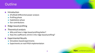
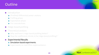
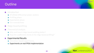
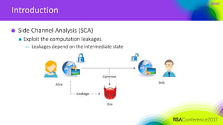
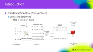
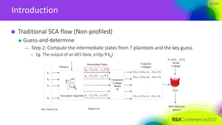
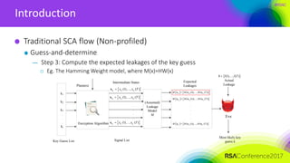
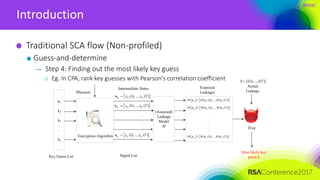
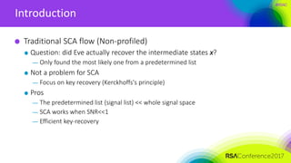
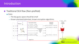
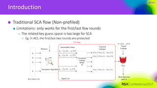
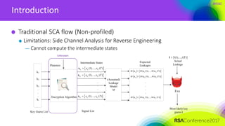
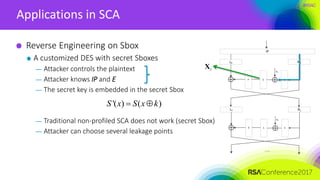
Introduction
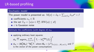
Notes on profiled attacks
Much stronger pre-conditions
— The Attacker gets an identical encryption device
Build templates
Perform template matching
— Works even if T=1 (in theory)
— Reverse the intermediate states without key guesses
Not always appropriate
— Power Variability Issues [Renauld, M., et al EUROCRYPT 2011]
We only focus on non-profiled attacks in this paper
Eve
Actual
Leakage
Most likely key
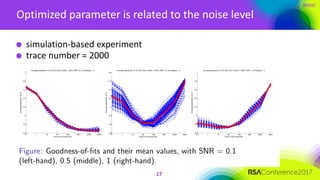
guess k
(1),..., ( )l l Tl
Intermediate States
Templates
Tp
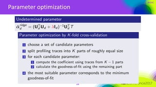
* * *
1 ,..., Tx x x](https://image.slidesharecdn.com/cryp-f01cryp-f01side-channel-analysis-170413122144/85/Ridge-based-Profiled-Differential-Power-Analysis-51-320.jpg)


![#RSAC
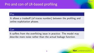
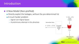
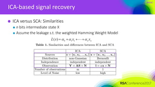
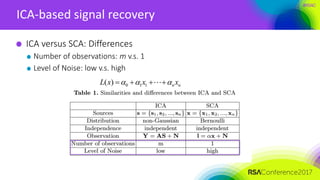
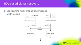
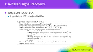
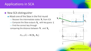
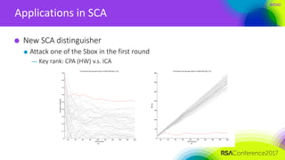
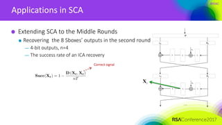
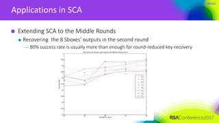
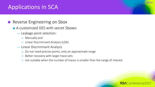
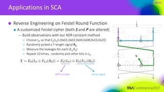
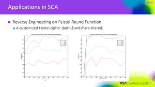
ICA-based signal recovery
Noise tolerance
Noise affects the performance of ICA
— ICA usually works in cases where SNR>>1
— For application in SCA, we need more robust algorithm
Ignored feature in ICA
— the distribution of the sources is given: binary signals
— the priori distribution can make ICA more robust to noise
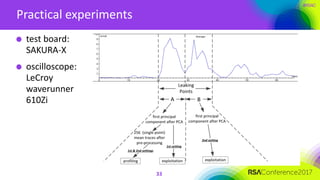
— EM-ICA: specialized for discrete sources with random noise, using Expectation-
Maximization algorithm [Belouchrouni, Cardoso 1994]](https://image.slidesharecdn.com/cryp-f01cryp-f01side-channel-analysis-170413122144/85/Ridge-based-Profiled-Differential-Power-Analysis-62-320.jpg)
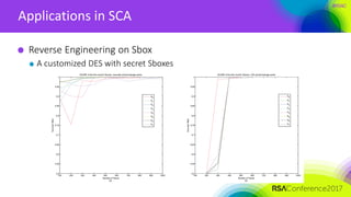


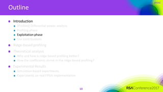
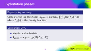
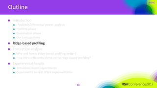
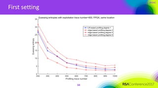
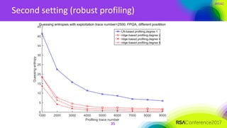
The document discusses ridge-based profiling in differential power analysis, outlining its theoretical advantages over traditional profiling methods. It describes the phases of profiling and exploitation and provides experimental results that highlight the effectiveness of ridge-based methods for reducing overfitting and improving performance in power analysis. Additionally, practical applications and comparisons with other profiling techniques are included, demonstrating the method's robustness and efficiency.


![Eloi Sanfelix - Hardware security: Side Channel Attacks [RootedCON 2011]](https://cdn.slidesharecdn.com/ss_thumbnails/esanfelix-sidechannelattacks-110307125844-phpapp01-thumbnail.jpg?width=640&height=640&fit=bounds)