This document provides an introduction to differential equations. It defines key concepts such as dependent and independent variables, ordinary and partial differential equations, order of a differential equation, and linearity. Examples of first order differential equations are given, including one modeling the motion of a falling body subject to gravity and air resistance. Differential equations arise in many areas of physics and applied mathematics, such as modeling the weather, electrical circuits, cooling objects, and population growth. The document outlines some basic types of differential equations that will be covered in subsequent chapters.

1. Introductory Differential Equations using
SAGE
David Joyner
11-22-2007

2. There are some things which cannot
be learned quickly, and time, which is all we have,
must be paid heavily for their acquiring.
They are the very simplest things,
and because it takes a man’s life to know them
the little new that each man gets from life
is very costly and the only heritage he has to leave.
Ernest Hemingway
(From A. E. Hotchner, Papa Hemingway, Random House, NY, 1966)

4. Contents
1 First order differential equations 1
1.1 Introduction to DEs . . . . . . . . . . . . . . . . . . . . . . . 1
1.2 Initial value problems . . . . . . . . . . . . . . . . . . . . . . . 10
1.3 First order ODEs - separable and linear cases . . . . . . . . . 15
1.4 Isoclines and direction fields . . . . . . . . . . . . . . . . . . . 24
1.5 Numerical solutions - Euler’s method and improved Euler’s
method . . . . . . . . . . . . . . . . . . . . . . . . . . . . . . 28
1.6 Newtonian mechanics . . . . . . . . . . . . . . . . . . . . . . . 38
1.7 Application to mixing problems . . . . . . . . . . . . . . . . . 44
2 Second order differential equations 49
2.1 Linear differential equations . . . . . . . . . . . . . . . . . . . 50
2.2 Linear differential equations, continued . . . . . . . . . . . . . 57
2.3 Undetermined coefficients method . . . . . . . . . . . . . . . . 63
2.3.1 Annihilator method . . . . . . . . . . . . . . . . . . . . 72
2.4 Variation of parameters . . . . . . . . . . . . . . . . . . . . . . 74
2.5 Applications of DEs: Spring problems . . . . . . . . . . . . . . 79
2.5.1 Part 1 . . . . . . . . . . . . . . . . . . . . . . . . . . . 79
2.5.2 Part 2 . . . . . . . . . . . . . . . . . . . . . . . . . . . 86
2.5.3 Part 3 . . . . . . . . . . . . . . . . . . . . . . . . . . . 90
2.6 Applications to simple LRC circuits . . . . . . . . . . . . . . . 93
2.7 The power series method . . . . . . . . . . . . . . . . . . . . . 99
2.7.1 Part 1 . . . . . . . . . . . . . . . . . . . . . . . . . . . 99
2.7.2 Part 2 . . . . . . . . . . . . . . . . . . . . . . . . . . . 106
2.8 The Laplace transform method . . . . . . . . . . . . . . . . . 112
2.8.1 Part 1 . . . . . . . . . . . . . . . . . . . . . . . . . . . 112
2.8.2 Part 2 . . . . . . . . . . . . . . . . . . . . . . . . . . . 120
vii

5. 3 Systems of first order differential equations 127
3.1 An introduction to systems of DEs: Lanchester’s equations . . 128
3.2 The Gauss elimination game and applications to systems of DEs133
3.3 Eigenvalue method for systems of DEs . . . . . . . . . . . . . 149
3.4 Electrical networks using Laplace transforms . . . . . . . . . . 159
4 Introduction to partial differential equations 165
4.1 Introduction to separation of variables . . . . . . . . . . . . . 165
4.2 Fourier series, sine series, cosine series . . . . . . . . . . . . . . 172
4.3 The heat equation . . . . . . . . . . . . . . . . . . . . . . . . 183
4.4 The wave equation in one dimension . . . . . . . . . . . . . . 195

6. Preface
The vast majority of this book comes from lecture notes I have been typing
up over the years for a could on differential equations with boundary value
problems at the USNA. Though the USNA is a government institution and
official work-related writing is in the public domain, I typed and polished
so much of this at home during the night and weekends that I feel I have
the right to claim copyright over this work. The DE course has used various
editions of the following three books (in order of most common use to least
common use) at various times:
• Dennis G. Zill and Michael R. Cullen, Differential equations with
Boundary Value Problems, 6th ed., Brooks/Cole, 2005.
• R. Nagle, E. Saff, and A. Snider, Fundamentals of Differential
Equations and Boundary Value Problems, 4th ed., Addison/Wesley,
2003.
• W. Boyce and R. DiPrima, Elementary Differential Equations and
Boundary Value Problems, 8th edition, John Wiley and Sons, 2005.
You may see some similarities but, for the most part, I have taught things a
bit differently and tried to impart this in these notes. Time will tell if there
are any improvements.
A new feature to this book is the fact that every section has at least one
SAGE exercise. SAGE is FOSS (free and open source software), available on
the most common computer platforms. Royalties for the sales of this book
(if it ever makes it’s way to a publisher) will go to further development of
SAGE .
This book is free and open source. It is licensed under the Attribution-
ShareAlike Creative Commons license, http: // creativecommons. org/ licenses/
by-sa/ 3. 0/ , or the Gnu Free Documentation License (GFDL), http:
// www. gnu. org/ copyleft/ fdl. html , at your choice.

7. Acknowledgments
In a few cases I have made use of the excellent (public domain!) lecture
notes by Sean Mauch,
Sean Mauch, Introduction to methods of Applied Mathematics,
http://www.its.caltech.edu/~sean/book/unabridged.html
I some cases, I have made use of the material on Wikipedia, this includes
both discussion and in a few cases, diagrams or graphics. This material is
licensed under the GFDL or the Attribution-ShareAlike Creative Commons
license. In any case, the amount used here probably falls under the “fair use”
clause.
Software used:
Most graphics was created using SAGE (http://www.sagemath.org/) and
GIMP http://www.gimp.org/ by the author. The circuit diagrams were
created using Dia http://www.gnome.org/projects/dia/ and GIMP http:
//www.gimp.org/ by the author. A few spring diagrams were taken from
Wikipedia. Of course, LaTeX was used for the typesetting. Many thanks to
the developers of these programs for these free tools.

8. Intro...
If people do not believe that mathematics is simple, it is only
because they do not realize how complicated life is.
- John von Neumann
To be written ...

9. Chapter 1
First order differential
equations
1.1 Introduction to DEs
But there is another reason for the high repute of mathe-
matics: it is mathematics that offers the exact natural sciences
a certain measure of security which, without mathematics, they
could not attain.
- Albert Einstein
Motivation
Roughly speaking, a differential equation is an equation involving the deriva-
tives of one or more unknown functions.
In calculus (differential, integral and vector), you’ve studied ways of ana-
lyzing functions. You might even have been convinced that functions you
meet in applications arise naturally from physical principles. As we shall
see, differential equations arise naturally from general physical principles. In
many cases, the functions you met in calculus in applications to physics were
actually solutions to a “natural” differential equation.
Example 1.1.1. Consider a falling body of mass m on which exactly 3 forces
act:
1

10. • gravitation, Fgrav ,
• air resistance, Fres ,
• an external force, Fext = f (t), where f (t) is some given function.
6
Fres Fgrav
mass m
?
Let x(t) denote the distance fallen from some fixed initial position. The
velocity is denoted by v = x′ and the acceleration by a = x′′ . We choose
an orientation so that downwards is positive. In this case, Fgrav = mg,
where g > 0 is the gravitational constant. We assume that air resistance is
proportional to velocity (a common assumption in physics), and write Fres =
−kv = −kx′ , where k > 0 is a “friction constant”. The total force, Ftotal , is
by hypothesis,
Ftotal = Fgrav + Fres + Fext ,
and, by Newton’s 2nd Law1 ,
Ftotal = ma = mx′′ .
Putting these together, we have
mx′′ = ma = mg − kx′ + f (t),
or
mx′′ + mx′ = f (t) + mg.
This is a differential equation in x = x(t). It may also be rewritten as a
differential equation in v = v(t) = x′ (t) as
1
“Force equals mass times acceleration.” http://en.wikipedia.org/wiki/Newtons_
law

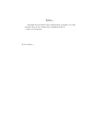
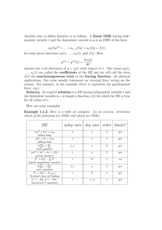
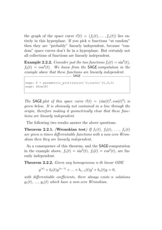
11. mv ′ + kv = f (t) + mg.
This is an example of a “first order differential equation in v”, which means
that at most first order derivatives of the unknown function v = v(t) occur.
In fact, you have probably seen solutions to this in your calculus classes, at
least when f (t) = 0 and k = 0. In that case, v ′ (t) = g and so v(t) = g dt =
gt + C. Here the constant of integration C represents the initial velocity.
Differential equations occur in other areas as well: weather prediction (more
generally, fluid-flow dynamics), electrical circuits, the heat of a homogeneous
wire, and many others (see the table below). They even arise in problems
on Wall Street: the Black-Scholes equation is a PDE which models the pric-
ing of derivatives [BS-intro]. Learning to solve differential equations helps
understand the behaviour of phenomenon present in these problems.
phenomenon description of DE
weather Navier-Stokes equation [NS-intro]
a non-linear vector-valued higher-order PDE
falling body 1st order linear ODE
motion of a mass attached Hooke’s spring equation
to a spring 2nd order linear ODE [H-intro]
motion of a plucked guitar string Wave equation
2nd order linear PDE [W-intro]
Battle of Trafalger Lanchester’s equations
system of 2 1st order DEs [L-intro], [M-intro], [N-intro]
cooling cup of coffee Newton’s Law of Cooling
in a room 1st order linear ODE
population growth logistic equation
non-linear, separable, 1st order ODE
Undefined terms and notation will be defined below, except for the equations
themselves. For those, see the references or wait until later sections when
they will be introduced2 .
Basic Concepts:
Here are some of the concepts to be introduced below:
2
Except for the Navier-Stokes equation, which is more complicated and might take us
too far afield.

12. • dependent variable(s),
• independent variable(s),
• ODEs,
• PDEs,
• order,
• linearity,
• solution.
It is really best to learn these concepts using examples. However, here are
the general definitions anyway, with examples to follow.
The term “differential equation” is sometimes abbreviated DE, for brevity.
Dependent/independent variables: Put simply, a differential equation
is an equation involving derivatives of one of more unknown functions. The
variables you are differentiating with respect to are the independent vari-
ables of the DE. The variables (the “unknown functions”) you are differenti-
ating are the dependent variables of the DE. Other variables which might
occur in the DE are sometimes called “parameters”.
ODE/PDE: If none of the derivatives which occur in the DE are partial
derivatives (for example, if the dependent variable/unknown function is a
function of a single variable) then the DE is called an ordinary differential
equation of PDE. If some of the derivatives which occur in the DE are
partial derivatives then the DE is a partial differential equation or PDE.
Order: The highest total number of derivatives you have to take in the
DE is it’s order.
Linearity: This can be described in a few different ways. First of all, a DE
is linear if the only operations you perform on its terms are combinations of
the following:
• differentiation with respect to independent variable(s),
• multiplication by a function of the independent variable(s).

13. Another way to define linearity is as follows. A linear ODE having inde-
pendent variable t and the dependent variable is y is an ODE of the form
a0 (t)y (n) + ... + an−1 (t)y ′ + an (t)y = f (t),
for some given functions a0 (t), . . . , an (t), and f (t). Here
dn y(t)
y (n) = y (n) (t) =
dtn
denotes the n-th derivative of y = y(t) with respect to t. The terms a0 (t),
. . . , an (t) are called the coefficients of the DE and we will call the term
f (t) the non-homogeneous term or the forcing function. (In physical
applications, this term usually represents an external force acting on the
system. For instance, in the example above it represents the gravitational
force, mg.)
Solution: An explicit solution to a DE having independent variable t and
the dependent variable is x is simple a function x(t) for which the DE is true
for all values of t.
Here are some examples:
Example 1.1.2. Here is a table of examples. As an exercise, determine
which of the following are ODEs and which are PDEs.
DE indep vars dep vars order linear?
mx′′ + kx′ = mg t x 2 yes
falling body
mv ′ + kv = mg t v 1 yes
falling body
2
k ∂ u = ∂u
∂x2 ∂t t, x u 2 yes
heat equation
mx′′ + bx′ + kx = f (t) t x 2 yes
spring equation
P
P ′ = k(1 − K )P t P 1 no
logistic population equation
2 2
k ∂ u = ∂ 2u
∂x2 ∂ t t, x u 2 yes
wave equation
T ′ = k(T − Troom ) t T 1 yes
Newton’s Law of Cooling
x′ = −Ay, y ′ = −Bx, t x, y 1 yes
Lanchester’s equations

14. Remark: Note that in many of these examples, the symbol used for the
independent variable is not made explicit. For example, we are writing x′
when we really mean x′ (t) = x(t) . This is very common shorthand notation
dt
and, in this situation, we shall usually use t as the independent variable
whenever possible.
Example 1.1.3. Recall a linear ODE having independent variable t and the
dependent variable is y is an ODE of the form
a0 (t)y (n) + ... + an−1 (t)y ′ + an (t)y = f (t),
for some given functions a0 (t), . . . , an (t), and f (t). The order of this DE is
n. In particular, a linear 1st order ODE having independent variable t and
the dependent variable is y is an ODE of the form
a0 (t)y ′ + a1 (t)y = f (t),
for some a0 (t), a1 (t), and f (t). We can divide both sides of this equation by
the leading coefficient a0 (t) without changing the solution y to this DE. Let’s
do that and rename the terms:
y ′ + p(t)y = q(t),
where p(t) = a1 (t)/a0 (t) and q(t) = f (t)/a0 (t). Every linear 1st order ODE
can be put into this form, for some p and q. For example, the falling body
equation mv ′ +kv = f (t)+mg has this form after dividing by m and renaming
v as y.
P
What does a differential equation like mx′′ + kx′ = mg or P ′ = k(1 − K )P
2u 2u
or k ∂ 2 = ∂ 2 t really mean? In mx′′ + kx′ = mg, m and k and g are given
∂x ∂
constants. The only things that can vary are t and the unknown function
x = x(t).
Example 1.1.4. To be specific, let’s consider x′ + x = 1. This means for all
t, x′ (t) + x(t) = 1. In other words, a solution x(t) is a function which, when
added to its derivative you always get the constant 1. How many functions
are there with that property? Try guessing a few “random” functions:
• √
Guess x(t) = sin(t). Compute (sin(t))′ + sin(t) = cos(t) + sin(t) =
2 sin(t + π ). x′ (t) + x(t) = 1 is false.
4

15. • Guess x(t) = exp(t) = et . Compute (et )′ + et = 2et . x′ (t) + x(t) = 1 is
false.
• Guess x(t) = exp(t) = t2 . Compute (t2 )′ + t2 = 2t + t2 . x′ (t) + x(t) = 1
is false.
• Guess x(t) = exp(−t) = e−t . Compute (e−t )′ +e−t = 0. x′ (t)+x(t) = 1
is false.
• Guess x(t) = exp(t) = 1. Compute (1)′ +1 = 0+1 = 1. x′ (t)+x(t) = 1
is true.
We finally found a solution by considering the constant function x(t) = 1.
Here a way of doing this kind of computation with the aid of the computer
algebra system SAGE :
SAGE
sage: t = var(’t’)
sage: de = lambda x: diff(x,t) + x - 1
sage: de(sin(t))
sin(t) + cos(t) - 1
sage: de(exp(t))
2*eˆt - 1
sage: de(tˆ2)
tˆ2 + 2*t - 1
sage: de(exp(-t))
-1
sage: de(1)
0
Note we have rewritten x′ + x = 1 as x′ + x − 1 = 0 and then plugged various
functions for x to see if we get 0 or not.
Obviously, we want a more systematic method for solving such equations
than guessing all the types of functions we know one-by-one. We will get to
those methods in time. First, we need some more terminology.
IVP: A first order initial value problem (abbreviated IVP) is a problem
of the form

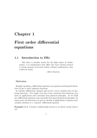
16. x′ = f (t, x), x(a) = c,
where f (t, x) is a given function of two variables, and a, c are given constants.
The equation x(a) = c is the initial condition.
Under mild conditions of f , an IVP has a solution x = x(t) which is unique.
This means that if f and a are fixed but c is a parameter then the solution
x = x(t) will depend on c. This is stated more precisely in the following
result.
Theorem 1.1.1. (Existence and uniqueness) Fix a point (t0 , x0 ) in the plane.
Let f (t, x) be a function of t and x for which both f (t, x) and fx (t, x) = ∂f∂x
(t,x)
are continuous on some rectangle
a < t < b, c < x < d,
in the plane. Here a, b, c, d are any numbers for which a < t0 < b and
c < x0 < d. Then there is an h > 0 and a unique solution x = x(t) for which
x′ = f (t, x), for all t ∈ (t0 − h, t0 + h),
and x(t0 ) = x0 .
This is proven in §2.8 of Boyce and DiPrima [BD-intro], but we shall not
prove this here. In most cases we shall run across, it is easier to construct
the solution than to prove this general theorem.
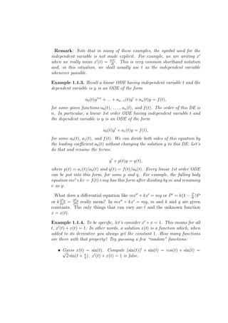
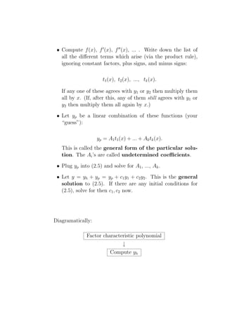
Example 1.1.5. Let us try to solve
x′ + x = 1, x(0) = 1.
The solutions to the DE x + x = 1 which we “guessed at” in the previous
′
example, x(t) = 1, satisfies this IVP.
Here a way of finding this slution with the aid of the computer algebra
system SAGE :
SAGE
sage: t = var(’t’)
sage: x = function(’x’, t)
sage: de = lambda y: diff(y,t) + y - 1
sage: desolve_laplace(de(x(t)),["t","x"],[0,1])
’1’

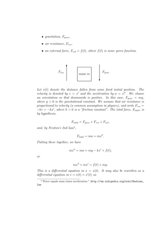
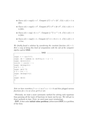
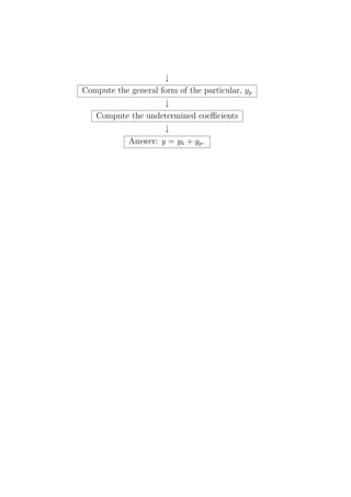
17. (The command desolve_laplace is a DE solver in SAGE which uses a special
method involving Laplace transforms which we will learn later.) Just as an
illustration, let’s try another example. Let us try to solve
x′ + x = 1, x(0) = 2.
The SAGE commands are similar:
SAGE
sage: t = var(’t’)
sage: x = function(’x’, t)
sage: de = lambda y: diff(y,t) + y - 1
sage: desolve_laplace(de(x(t)),["t","x"],[0,2])
’%eˆ-t+1’
age: solnx = lambda s: RR(eval(soln.replace("ˆ","**").
replace("%","").replace("t",str(s))))
sage: solnx(3)
1.04978706836786
sage: P = plot(solnx,0,5)
sage: show(P)
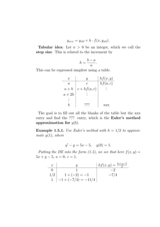
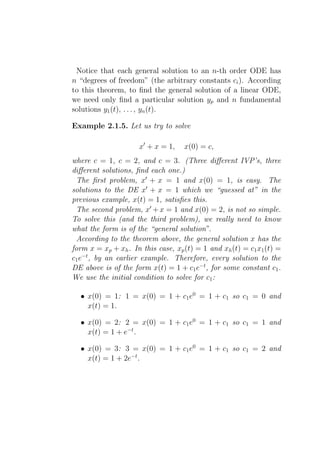
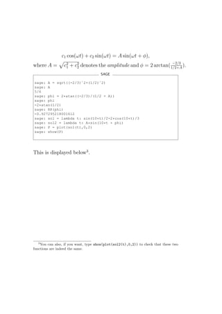
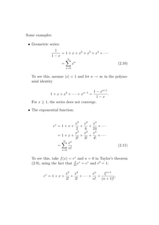
The plot is given below.
Figure 1.1: Solution to IVP x′ + x = 1, x(0) = 2.

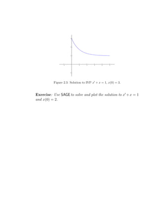
18. Exercise: Verify the, for any constant c, the function x(t) = 1 + ce−t solves
x′ + x = 1. Find the c for which this function solves the IVP x′ + x = 1,
x(0) = 3.. Solve this (a) by hand, (b) using SAGE .
1.2 Initial value problems
A 1-st order initial value problem, or IVP, is simply a 1-st order ODE
and an initial condition. For example,
x′ (t) + p(t)x(t) = q(t), x(0) = x0 ,
where p(t), q(t) and x0 are given. The analog of this for 2nd order linear
DEs is this:
a(t)x′′ (t) + b(t)x′ (t) + c(t)x(t) = f (t), x(0) = x0 , x′ (0) = v0 ,
where a(t), b(t), c(t), x0 , and v0 are given. This 2-nd order linear DE and
initial conditions is an example of a 2-nd order IVP. In general, in an IVP,
the number of initial conditions must match the order of the DE.
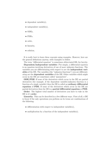
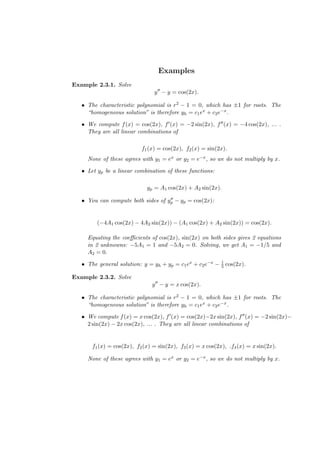
Example 1.2.1. Consider the 2-nd order DE
x′′ + x = 0.
(We shall run across this DE many times later. As we will see, it represents
the displacement of an undamped spring with a unit mass attached. The term
harmonic oscillator is attached to this situation [O-ivp].) Suppose we know
that the general solution to this DE is
x(t) = c1 cos(t) + c2 sin(t),
for any constants c1 , c2 . This means every solution to the DE must be of this
form. (If you don’t believe this, you can at least check it it is a solution by
computing x′′ (t)+x(t) and verifying that the terms cancel, as in the following
SAGE example. Later, we see how to derive this solution.) Note that there
are two degrees of freedom (the constants c1 and c2 ), matching the order of
the DE.
SAGE
sage: t = var(’t’)

19. sage: c1 = var(’c1’)
sage: c2 = var(’c2’)
sage: de = lambda x: diff(x,t,t) + x
sage: de(c1*cos(t) + c2*sin(t))
0
sage: x = function(’x’, t)
sage: soln = desolve_laplace(de(x(t)),["t","x"],[0,0,1])
sage: soln
’sin(t)’
sage: solnx = lambda s: RR(eval(soln.replace("t","s")))
sage: P = plot(solnx,0,2*pi)
sage: show(P)
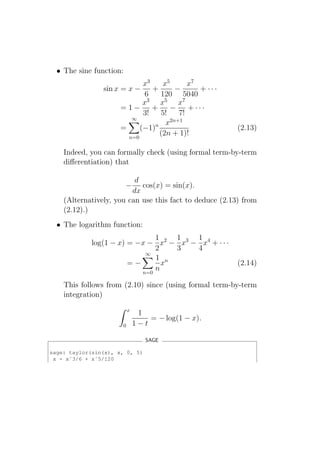
This is displayed below.
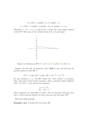
Now, to solve the IVP
x′′ + x = 0, x(0) = 0, x′ (0) = 1.
the problem is to solve for c1 and c2 for which the x(t) satisfies the initial
conditions. The two degrees of freedom in the general solution matching the
number of initial conditions in the IVP. Plugging t = 0 into x(t) and x′ (t),
we obtain
0 = x(0) = c1 cos(0) + c2 sin(0) = c1 , 1 = x′ (0) = −c1 sin(0) + c2 cos(0) = c2 .
Therefore, c1 = 0, c2 = 1 and x(t) = sin(t) is the unique solution to the IVP.
Figure 1.2: Solution to IVP x′′ + x = 0, x(0) = 0, x′ (0) = 1.
Here you see the solution oscillates, as t gets larger.

20. Another example,
Example 1.2.2. Consider the 2-nd order DE
x′′ + 4x′ + 4x = 0.
(We shall run across this DE many times later as well. As we will see, it
represents the displacement of a critially damped spring with a unit mass
attached.) Suppose we know that the general solution to this DE is
x(t) = c1 exp(−2t) + c2 texp(−2t) = c1 e−2t + c2 te−2t ,
for any constants c1 , c2 . This means every solution to the DE must be of
this form. (Again, you can at least check it is a solution by computing x′′ (t),
4x′ (t), 4x(t), adding them up and verifying that the terms cancel, as in the
following SAGE example.)
SAGE
sage: t = var(’t’)
sage: c1 = var(’c1’)
sage: c2 = var(’c2’)
sage: de = lambda x: diff(x,t,t) + 4*diff(x,t) + 4*x
sage: de(c1*exp(-2*t) + c2*t*exp(-2*t))
4*(c2*t*eˆ(-2*t) + c1*eˆ(-2*t)) + 4*(-2*c2*t*eˆ(-2*t)
+ c2*eˆ(-2*t) - 2*c1*eˆ(-2*t)) + 4*c2*t*eˆ(-2*t)
- 4*c2*eˆ(-2*t) + 4*c1*eˆ(-2*t)
sage: de(c1*exp(-2*t) + c2*t*exp(-2*t)).expand()
0
sage: desolve_laplace(de(x(t)),["t","x"],[0,0,1])
’t*%eˆ-(2*t)’
sage: P = plot(t*exp(-2*t),0,pi)
sage: show(P)
The plot is displayed below.
Now, to solve the IVP
x′′ + 4x′ + 4x = 0, x(0) = 0, x′ (0) = 1.
we solve for c1 and c2 using the initial conditions. Plugging t = 0 into x(t)
and x′ (t), we obtain

21. 0 = x(0) = c1 exp(0) + c2 · 0 · exp(0) = c1 ,
1 = x′ (0) = c1 exp(0) + c2 exp(0) − 2c2 · 0 · exp(0) = c1 + c2 .
Therefore, c1 = 0, c1 + c2 = 1 and so x(t) = t exp(−2t) is the unique solution
to the IVP. Here you see the solution tends to 0, as t gets larger.
Figure 1.3: Solution to IVP x′′ + 4x′ + 4x = 0, x(0) = 0, x′ (0) = 1.
Suppose, for the sake of argument, that I lied to you and told you the
general solution to this DE is
x(t) = c1 exp(−2t) + c2 exp(−2t) = c1 (e−2t + c2 e−2t ),
for any constants c1 , c2 . (In other words, the “extra t factor” is missing.)
Now, if you try to solve for the constant c1 and c2 using the initial conditions
x(0) = 0, x′ (0) = 1 you will get the equations
c1 + c2 = 0
−2c1 − 2c2 = 1.
These equations are impossible to solve! You see from this that you must
have a correct general solution to insure that you can solve your IVP.
One more quick example.
Example 1.2.3. Consider the 2-nd order DE

22. x′′ − x = 0.
Suppose we know that the general solution to this DE is
x(t) = c1 exp(t) + c2 exp(−t) = c1 e−t + c2 e−t ,
for any constants c1 , c2 . (Again, you can check it is a solution.)
The solution to the IVP
x′′ − x = 0, x(0) = 0, x′ (0) = 1,
t
is x(t) = e +e . (You can solve for c1 and c2 yourself, as in the examples
−t
2
above.) This particular function is also called a hyperbolic cosine func-
tion, denoted cosh(t).
The hyperbolic trig functions have many properties analogous to the usual
trig functions and arise in many areas of applications [H-ivp]. For example,
cosh(t) represents a catenary or hanging cable [C-ivp].
SAGE
sage: t = var(’t’)
sage: c1 = var(’c1’)
sage: c2 = var(’c2’)
sage: de = lambda x: diff(x,t,t) - x
sage: de(c1*exp(-t) + c2*exp(-t))
0
sage: desolve_laplace(de(x(t)),["t","x"],[0,0,1])
’%eˆt/2-%eˆ-t/2’
sage: P = plot(eˆt/2-eˆ(-t)/2,0,3)
sage: show(P)
Here you see the solution tends to infinity, as t gets larger.
Exercise: The general solution to the falling body problem
mv ′ + kv = mg,
is v(t) = mg + ce−kt/m . If v(0) = v0 , solve for c in terms of v0 . Take
k
m = k = v0 = 1, g = 9.8 and use SAGE to plot v(t) for 0 < t < 1.

23. Figure 1.4: Solution to IVP x′′ − x = 0, x(0) = 0, x′ (0) = 1.
1.3 First order ODEs - separable and linear
cases
Separable DEs:
We know how to solve any ODE of the form
y ′ = f (t),
at least in principle - just integrate both sides3 . For a more
general type of ODE, such as
y ′ = f (t, y),
this fails. For instance, if y ′ = t + y then integrating both sides
gives y(t) = dy dt = y ′ dt = t + y dt = t dt + y(t) dt =
dt
3
Recall y ′ really denotes dy , so by the fundamental theorem of calculus, y = dy dt =
dt dt
′
y dt = f (t) dt = F (t) + c, where F is the “anti-derivative” of f and c is a constant of
integration.

24. t2
2+ y(t) dt. So, we have only succeeded in writing y(t) in terms
of its integral. Not helpful.
However, there is a class of ODEs where this idea works, with
some slight modification. If the ODE has the form
g(t)
y′ = , (1.1)
h(y)
then it is called separable4 .
To solve a separable ODE:
dy g(t)
(1) write the ODE (1.1) as dt = h(y) ,
(2) “separate” the t’s and the y’s:
h(y) dy = g(t) dt,
(3) integrate both sides:
h(y) dy = g(t) dt + C
I’ve added a “+C” to emphasize that a constant of inte-
gration must be included in your anwser (but only on one
side of the equation).
The answer obtained in this manner is called an “implicit so-
lution” of (1.1) since it expresses y implicitly as a function of
t.
Example 1.3.1. Are the following ODEs separable? If so, solve
them.
4
It particular, any separable DE must be first order.

25. (a) (t2 + y 2 )y ′ = −2ty,
(b) y ′ = −x/y, y(0) = −1,
(c) T ′ = k · (T − Troom ), where k < 0 and Troom are constants,
(d) ax′ + bx = c, where a = 0, b = 0, and c are constants
(e) ax′ + bx = c, where a = 0, b, are constants and c = c(t) is
not a constant.
(f ) y ′ = (y − 1)(y + 1), y(0) = 2.
(g) y ′ = y 2 + 1, y(0) = 1.
Solutions:
(a) not separable,
(b) y dy = −x dx, so y 2 /2 = −x2 /2 + c, so x2 + y 2 = 2c. This
is the general solution (note it does not give y explicitly as
a function of x, you will have to solve for y algebraically to
get that). The initial conditions say when x = 0, y = 1,
so 2c = 02 + 12 = 1, which gives c = 1/2. Therefore,
x2 + y 2 = 1, which is a circle. That is not a function
so cannot be the solution √ want. The solution is either
√ we
y = 1−x 2 or y = − 1 − x2 , but which one? Since
√
y(0) = −1 (note the minus sign) it must be y = − 1 − x2 .
dT
(c) T −Troom= kdt, so ln |T − Troom | = kt + c (some constant
c), so T − Troom = Cekt (some constant C), so T = T (t) =
Troom + Cekt .

26. dx
(d) dt = (c−bx)/a = − a (x− c ), so
b
b
dx
x− c
b
= − a dt, so ln |x− c | =
b
b
b
− a t + C, where C is a constant of integration. This is the
implicit general solution of the DE. The explicit general
b
solution is x = c + Be− a t , where B is a constant.
b
The explicit solution is easy find using SAGE :
SAGE
sage: a = var(’a’)
sage: b = var(’b’)
sage: c = var(’c’)
sage: t = var(’t’)
sage: x = function(’x’, t)
sage: de = lambda y: a*diff(y,t) + b*y - c
sage: desolve_laplace(de(x(t)),["t","x"])
’c/b-(a*c-x(0)*a*b)*%eˆ-(b*t/a)/(a*b)’
(e) If c = c(t) is not constant then ax′ +bx = c is not separable.
dy 1
(f ) (y−1)(y+1)= dt so 2 (ln(y − 1) − ln(y + 1)) = t + C, where C
is a constant of integration. This is the “general (implicit)
solution” of the DE.
Note: the constant functions y(t) = 1 and y(t) = −1 are
also solutions to this DE. These solutions cannot be ob-
tained (in an obvious way) from the general solution.
The integral is easy to do using SAGE :
SAGE
sage: y = var(’y’)
sage: integral(1/((y-1)*(y+1)),y)
log(y - 1)/2 - (log(y + 1)/2)

27. Now, let’s try to get SAGE to solve for y in terms of t in
1
2 (ln(y − 1) − ln(y + 1)) = t + C:
SAGE
sage: C = var(’C’)
sage: solve([log(y - 1)/2 - (log(y + 1)/2) == t+C],y)
[log(y + 1) == -2*C + log(y - 1) - 2*t]
This is not working. Let’s try inputting the problem in a
different form:
SAGE
sage: C = var(’C’)
sage: solve([log((y - 1)/(y + 1)) == 2*t+2*C],y)
[y == (-eˆ(2*C + 2*t) - 1)/(eˆ(2*C + 2*t) - 1)]
This is what we want. Now let’s assume the initial condi-
tion y(0) = 2 and solve for C and plot the function.
SAGE
sage: solny=lambda t:(-eˆ(2*C+2*t)-1)/(eˆ(2*C+2*t)-1)
sage: solve([solny(0) == 2],C)
[C == log(-1/sqrt(3)), C == -log(3)/2]
sage: C = -log(3)/2
sage: solny(t)
(-eˆ(2*t)/3 - 1)/(eˆ(2*t)/3 - 1)
sage: P = plot(solny(t), 0, 1/2)
sage: show(P)

28. This plot is shown below. The solution has a singularity at
t = ln(3)/2 = 0.5493....
Figure 1.5: Plot of y ′ = (y − 1)(y + 1), y(0) = 2, for 0 < t < 1/2..
dy
(g) = dt so arctan(y) = t + C, where C is a constant of
y 2 +1
integration. The initial condition y(0) = 1 says arctan(1) =
C, so C = π . Therefore y = tan(t + π ) is the solution.
4 4
A special subclass of separable ODEs is the class of automo-
mous ODEs, which have the form
y ′ = f (y),
where f is a given function (i.e., the slope y only depends on
the value of the dependent variable y). The cases (c), (d), (f),
and (g) above are examples.
Linear 1st order DEs:
The bottom line is that we want to solve any problem of the
form

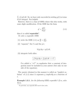
29. x′ + p(t)x = q(t), (1.2)
where p(t) and q(t) are given functions (which, let’s assume,
aren’t too horrible). Every first order linear ODE can be writ-
ten in this form. Examples of DEs which have this form: Falling
Body problems, Newton’s Law of Cooling problems, Mixing
problems, certain simple Circuit problems, and so on.
There are two approaches
• “the formula”,
• the method of integrating factors.
Both lead to the exact same solution.
“The Formula”: The general solution to (1.2) is
p(t) dt
e q(t) dt + C
x= , (1.3)
e p(t) dt
where C is a constant. The factor e p(t) dt is called the inte-
grating factor and is often denoted by µ. This formula was
apparently first discovered by Johann Bernoulli [F-1st].
Example 1.3.2. Solve
xy ′ + y = ex .
x 1
1
We rewrite this as y ′ + x y = ex . Now compute µ = e x dx
=
eln(x) = x, so the formula gives
x
x ex dx + C ex dx + C ex + C
y= = = .
x x x
Here is one way to do this using SAGE :

30. SAGE
sage: t = var(’t’)
sage: x = function(’x’, t)
sage: de = lambda y: diff(y,t) + (1/t)*y - exp(t)/t
sage: desolve(de(x(t)),[x,t])
’(%eˆt+%c)/t’
p(t) dt
“Integrating factor method”: Let µ = e . Multiply both
sides of (1.2) by µ:
µx′ + p(t)µx = µq(t).
The product rule implies that
(µx)′ = µx′ + p(t)µx = µq(t).
(In response to a question you are probably thinking now: No,
this is not obvious. This is Bernoulli’s very clever idea.) Now
just integrate both sides. By the fundamental theorem of calcu-
lus,
µx = (µx)′ dt = µq(t) dt.
Dividing both side by µ gives (1.3).

31. Exercise: (a) Use SAGE ’s desolve command to solve
tx′ + 2x = et /t.
(b) Use SAGE to plot the solution to y ′ = y 2 − 1, y(0) = −2.

32. 1.4 Isoclines and direction fields
Recall from vector calculus the notion of a two-dimensional vec-
tor field: F (x, y) = (g(x, y), h(x, y)). To plot F , you simply
draw the vector F (x, y) at each point (x, y).
The idea of the direction field (or slope field) associated to
the first order ODE
y ′ = f (x, y), y(a) = c, (1.4)
is similar. At each point (x, y) you plot a vector having slope
f (x, y). For example, the vector field plot of F (x, y) = (1, f (x, y))
or F (x, y) = (1, f (x, y))/ 1 + f (x, y)2 (which is a unit vector).
A related notion are the isoclines of the ODE. An isocline of
(1.4) is a level curve of the function z = f (x, y):
{(x, y) | f (x, y) = m},
where the given constant m is called the slope of the isocline. In
terms of the ODE, this curve represents the collection of points
at which the solution has slope m. In terms of the direction
field of the ODE, it represents the collection of points where the
vectors have slope m.
How to draw the direction field of (1.4) by hand:
• Draw several isoclines, making sure to include one which
contains the point (a, c). (You may want to draw these in
pencil.)
• On each isocline, draw “hatch marks” or “arrows” along
the line each having slope m.

33. This is a crude direction field plot. The plot of arrows form
your direction field. The isoclines, having served their useful-
ness, can safely be ignored or erased.
Example 1.4.1. The direction field, with three isoclines, for
y ′ = 5x + y − 5, y(0) = 1,
is given by the following graph:
Figure 1.6: Plot of y ′ = 5x + y − 5, y(0) = 1, for −1 < x < 1.
The isoclines are the curves (coincidentally, lines) of the form
5x + y − 5 = m. (They are green bands in the above plot.) These
are lines of slope −5, not to be confused with the fact that it
represents an isocline of slope m.
The above example can be solved explicitly. (Indeed, y =
−5x + ex solves y ′ = 5x + y − 5, y(0) = 1.) In the next example,
such an explicit solution is (as far as I know), not possible.
Therefore, a numerical approximation plays a more important
role.

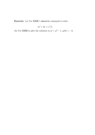
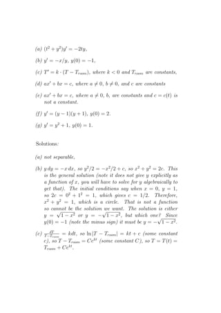
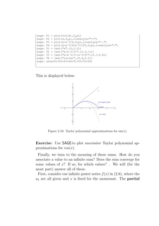
34. Example 1.4.2. The direction field, with three isoclines, for
y ′ = x2 + y 2 , y(0) = 3/2,
is given by the following graph:
Figure 1.7: Direction field and solution plot of y ′ = x2 + y 2 , y(0) = 3/2, for
−3 < x < 3.
The isoclines are the concentric circles x2 + y 2 = m. (They are
green in the above plot.)
The plot above was obtained using SAGE ’s interface with Max-
ima, and the plotting package Openmath (SAGE includes both
Maxima and Openmath). :
SAGE
sage: maxima.eval(’load("plotdf")’)
sage: maxima.eval(’plotdf(xˆ2+yˆ2,[trajectory_at,0,0],
[x,-3,3],[y,-3,3])’)
This gave the above plot. (Note: the plotdf command goes on
one line; for typographical reasons, it was split in two.)

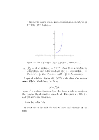
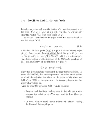
35. There is also a way to draw these direction fields using SAGE .
SAGE
sage: pts = [(-2+i/5,-2+j/5) for i in range(20)
for j in range(20)] # square [-2,2]x[-2,2]
sage: f = lambda p:p[0]ˆ2+p[1]ˆ2
sage: arrows = [arrow(p, (p[0]+0.02,p[1]+(0.02)*f(p)),
width=1/100, rgbcolor=(0,0,1)) for p in pts]
sage: show(sum(arrows))
This gives the plot below.
Figure 1.8: Direction field for y ′ = x2 + y 2 , y(0) = 3/2, for −2 < x < 2.
Exercise: Using SAGE , plot the direction field for y ′ = x2 − y 2 .

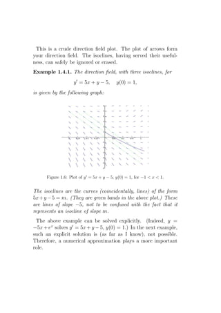
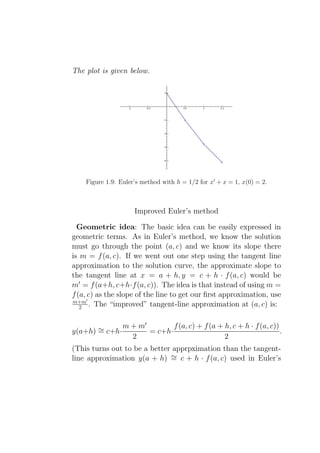
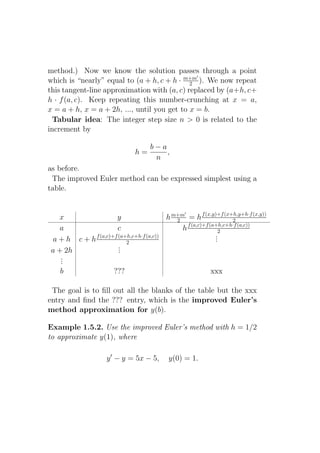
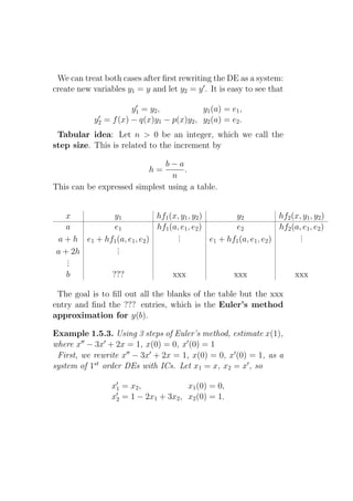
36. 1.5 Numerical solutions - Euler’s method and
improved Euler’s method
Read Euler: he is our master in everything.
- Pierre Simon de Laplace
Leonhard Euler was a Swiss mathematician who made signifi-
cant contributions to a wide range of mathematics and physics
including calculus and celestial mechanics (see [Eu1-num] and
[Eu2-num] for further details).
The goal is to find an approximate solution to the problem
y ′ = f (x, y), y(a) = c, (1.5)
where f (x, y) is some given function. We shall try to approxi-
mate the value of the solution at x = b, where b > a is given.
Sometimes such a method is called “numerically integrating
(1.5)”.
Note: the first order DE must be in the form (1.5) or the
method described below does not work. A version of Euler’s
method for systems of 1-st order DEs and higher order DEs will
also be described below.
Euler’s method
Geometric idea: The basic idea can be easily expressed in
geometric terms. We know the solution, whatever it is, must go
through the point (a, c) and we know, at that point, its slope is

37. m = f (a, c). Using the point-slope form of a line, we conclude
that the tangent line to the solution curve at (a, c) is (in (x, y)-
coordinates, not to be confused with the dependent variable y
and independent variable x of the DE)
y = c + (x − a)f (a, c).
In particular, if h > 0 is a given small number (called the in-
crement) then taking x = a+h the tangent-line approximation
from calculus I gives us:
y(a + h) ∼ c + h · f (a, c).
=
Now we know the solution passes through a point which is
“nearly” equal to (a + h, c + h · f (a, c). We now repeat this
tangent-line approximation with (a, c) replaced by (a + h, c +
h · f (a, c). Keep repeating this number-crunching at x = a,
x = a + h, x = a + 2h, ..., until you get to x = b.
Algebraic idea: The basic idea can also be explained “alge-
braically”. Recall from the definition of the derivative in calculus
1 that
y(x + h) − y(x)
y ′ (x) ∼
= ,
h
h > 0 is a given and small. This an the DE together give
f (x, y(x)) ∼ y(x+h)−y(x) . Now solve for y(x + h):
= h
y(x + h) ∼ y(x) + h · f (x, y(x)).
=
If we call h·f (x, y(x)) the “correction term” (for lack of anything
better), call y(x) the “old value of y”, and call y(x+h) the “new
value of y”, then this approximation can be re-expressed

38. ynew = yold + h · f (x, yold ).
Tabular idea: Let n > 0 be an integer, which we call the
step size. This is related to the increment by
b−a
h= .
n
This can be expressed simplest using a table.
x y hf (x, y)
a c hf (a, c)
.
.
a + h c + hf (a, c) .
.
.
a + 2h .
.
.
.
b ??? xxx
The goal is to fill out all the blanks of the table but the xxx
entry and find the ??? entry, which is the Euler’s method
approximation for y(b).
Example 1.5.1. Use Euler’s method with h = 1/2 to approxi-
mate y(1), where
y ′ − y = 5x − 5, y(0) = 1.
Putting the DE into the form (1.5), we see that here f (x, y) =
5x + y − 5, a = 0, c = 1.
x y hf (x, y) = 5x+y−5
2
0 1 −2
1/2 1 + (−2) = −1 −7/4
1 −1 + (−7/4) = −11/4

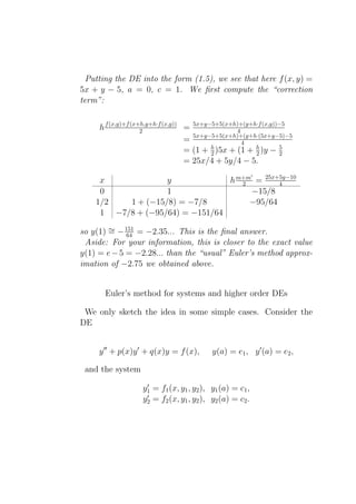
39. so y(1) ∼ − 11 = −2.75. This is the final answer.
= 4
Aside: For your information, y = ex − 5x solves the DE and
y(1) = e − 5 = −2.28....
Here is one way to do this using SAGE :
SAGE
sage: x,y=PolynomialRing(QQ,2,"xy").gens()
sage: eulers_method(5*x+y-5,1,1,1/3,2)
x y h*f(x,y)
1 1 1/3
4/3 4/3 1
5/3 7/3 17/9
2 38/9 83/27
sage: eulers_method(5*x+y-5,0,1,1/2,1,method="none")
[[0, 1], [1/2, -1], [1, -11/4], [3/2, -33/8]]
sage: pts = eulers_method(5*x+y-5,0,1,1/2,1,method="none")
sage: P = list_plot(pts)
sage: show(P)
sage: P = line(pts)
sage: show(P)
sage: P1 = list_plot(pts)
sage: P2 = line(pts)
sage: show(P1+P2)

40. The plot is given below.
Figure 1.9: Euler’s method with h = 1/2 for x′ + x = 1, x(0) = 2.
Improved Euler’s method
Geometric idea: The basic idea can be easily expressed in
geometric terms. As in Euler’s method, we know the solution
must go through the point (a, c) and we know its slope there
is m = f (a, c). If we went out one step using the tangent line
approximation to the solution curve, the approximate slope to
the tangent line at x = a + h, y = c + h · f (a, c) would be
m′ = f (a+h, c+h·f (a, c)). The idea is that instead of using m =
f (a, c) as the slope of the line to get our first approximation, use
m+m′
2 . The “improved” tangent-line approximation at (a, c) is:
m + m′ f (a, c) + f (a + h, c + h · f (a, c))
y(a+h) ∼ c+h·
= = c+h· .
2 2
(This turns out to be a better apprpximation than the tangent-
line approximation y(a + h) ∼ c + h · f (a, c) used in Euler’s
=

41. method.) Now we know the solution passes through a point
′
which is “nearly” equal to (a + h, c + h · m+m ). We now repeat
2
this tangent-line approximation with (a, c) replaced by (a+h, c+
h · f (a, c). Keep repeating this number-crunching at x = a,
x = a + h, x = a + 2h, ..., until you get to x = b.
Tabular idea: The integer step size n > 0 is related to the
increment by
b−a
h= ,
n
as before.
The improved Euler method can be expressed simplest using a
table.
h m+m = h f (x,y)+f (x+h,y+h·f (x,y))
′
x y 2 2
f (a,c)+f (a+h,c+h·f (a,c))
a c h 2
f (a,c)+f (a+h,c+h·f (a,c)) .
.
a+h c+h 2 .
.
.
a + 2h .
.
.
.
b ??? xxx
The goal is to fill out all the blanks of the table but the xxx
entry and find the ??? entry, which is the improved Euler’s
method approximation for y(b).
Example 1.5.2. Use the improved Euler’s method with h = 1/2
to approximate y(1), where
y ′ − y = 5x − 5, y(0) = 1.

42. Putting the DE into the form (1.5), we see that here f (x, y) =
5x + y − 5, a = 0, c = 1. We first compute the “correction
term”:
h f (x,y)+f (x+h,y+h·f (x,y)) = 5x+y−5+5(x+h)+(y+h·f (x,y))−5
2 4
5x+y−5+5(x+h)+(y+h·(5x+y−5)−5
= 4
= (1 + h )5x + (1 + h )y − 5
2 2 2
= 25x/4 + 5y/4 − 5.
′
x y h m+m = 25x+5y−10
2 4
0 1 −15/8
1/2 1 + (−15/8) = −7/8 −95/64
1 −7/8 + (−95/64) = −151/64
so y(1) ∼ − 151 = −2.35... This is the final answer.
= 64
Aside: For your information, this is closer to the exact value
y(1) = e − 5 = −2.28... than the “usual” Euler’s method approx-
imation of −2.75 we obtained above.
Euler’s method for systems and higher order DEs
We only sketch the idea in some simple cases. Consider the
DE
y ′′ + p(x)y ′ + q(x)y = f (x), y(a) = e1 , y ′ (a) = e2 ,
and the system
′
y1 = f1 (x, y1 , y2 ), y1 (a) = c1 ,
′
y2 = f2 (x, y1 , y2 ), y2 (a) = c2 .

43. We can treat both cases after first rewriting the DE as a system:
create new variables y1 = y and let y2 = y ′ . It is easy to see that
′
y1 = y2 , y1 (a) = e1 ,
′
y2 = f (x) − q(x)y1 − p(x)y2 , y2 (a) = e2 .
Tabular idea: Let n > 0 be an integer, which we call the
step size. This is related to the increment by
b−a
h= .
n
This can be expressed simplest using a table.
x y1 hf1 (x, y1 , y2 ) y2 hf2 (x, y1 , y2 )
a e1 hf1 (a, e1 , e2 ) e2 hf2 (a, e1 , e2 )
.
. .
.
a + h e1 + hf1 (a, e1 , e2 ) . e1 + hf1 (a, e1 , e2 ) .
.
.
a + 2h .
.
.
.
b ??? xxx xxx xxx
The goal is to fill out all the blanks of the table but the xxx
entry and find the ??? entries, which is the Euler’s method
approximation for y(b).
Example 1.5.3. Using 3 steps of Euler’s method, estimate x(1),
where x′′ − 3x′ + 2x = 1, x(0) = 0, x′ (0) = 1
First, we rewrite x′′ − 3x′ + 2x = 1, x(0) = 0, x′ (0) = 1, as a
system of 1st order DEs with ICs. Let x1 = x, x2 = x′ , so
′
x1 = x2 , x1 (0) = 0,
′
x2 = 1 − 2x1 + 3x2 , x2 (0) = 1.

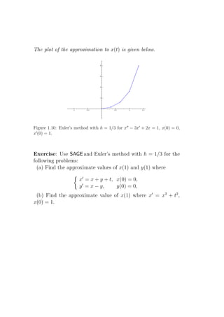
44. This is the DE rewritten as a system in standard form. (In
general, the tabular method applies to any system but it must be
in standard form.)
Taking h = (1 − 0)/3 = 1/3, we have
t x1 x2 /3 x2 (1 − 2x1 + 3x2 )/3
0 0 1/3 1 4/3
1/3 1/3 7/9 7/3 22/9
2/3 10/9 43/27 43/9 xxx
1 73/27 xxx xxx xxx
So x(1) = x1 (1) ∼ 73/27 = 2.7....
Here is one way to do this using SAGE :
SAGE
sage: RR = RealField(sci_not=0, prec=4, rnd=’RNDU’)
sage: t, x, y = PolynomialRing(RR,3,"txy").gens()
sage: f = y; g = 1-2*x+3*y
sage: L = eulers_method_2x2(f,g,0,0,1,1/3,1,method="none")
sage: L
[[0, 0, 1], [1/3, 0.35, 2.5], [2/3, 1.3, 5.5],
[1, 3.3, 12], [4/3, 8.0, 24]]
sage: eulers_method_2x2(f,g, 0, 0, 1, 1/3, 1)
t x h*f(t,x,y) y h*g(t,x,y)
0 0 0.35 1 1.4
1/3 0.35 0.88 2.5 2.8
2/3 1.3 2.0 5.5 6.5
1 3.3 4.5 12 11
sage: P1 = list_plot([[p[0],p[1]] for p in L])
sage: P2 = line([[p[0],p[1]] for p in L])
sage: show(P1+P2)

45. The plot of the approximation to x(t) is given below.
Figure 1.10: Euler’s method with h = 1/3 for x′′ − 3x′ + 2x = 1, x(0) = 0,
x′ (0) = 1.
Exercise: Use SAGE and Euler’s method with h = 1/3 for the
following problems:
(a) Find the approximate values of x(1) and y(1) where
x′ = x + y + t, x(0) = 0,
y ′ = x − y, y(0) = 0,
(b) Find the approximate value of x(1) where x′ = x2 + t2 ,
x(0) = 1.

46. 1.6 Newtonian mechanics
We briefly recall how the physics of the falling body problem
leads naturally to a differential equation (this was already men-
tioned in the introduction and forms a part of Newtonian me-
chanics [M-mech]). Consider a mass m falling due to gravity.
We orient coordinates to that downward is positive. Let x(t)
denote the distance the mass has fallen at time t and v(t) its
velocity at time t. We assume only two forces act: the force due
to gravity, Fgrav , and the force due to air resistence, Fres . In
other words, we assume that the total force is given by
Ftotal = Fgrav + Fres .
We know that Fgrav = mg, where g > 0 is the gravitational
constant, from high school physics. We assume, as is common
in physics, that air resistance is proportional to velocity: Fres =
−kv = −kx′ (t), where k ≥ 0 is a constant. Newton’s second
law [N-mech] tells us that Ftotal = ma = mx′′ (t). Putting these
all together gives mx′′ (t) = mg − kx′ (t), or
k
v ′ (t) + v(t) = g. (1.6)
m
This is the differential equation governing the motion of a falling
body. Equation (1.6) can be solved by various methods: separa-
tion of variables or by integrating factors. If we assume v(0) = v0
is given and if we assume k > 0 then the solution is
mg mg −kt/m
v(t) = + (v0 − )e . (1.7)
k k
In particular, we see that the limiting velocity is vlimit = mg .
k

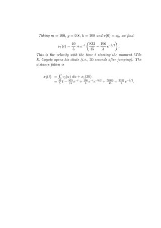
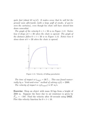
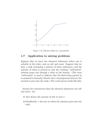
47. Example 1.6.1. Wile E. Coyote (see [W-mech] if you haven’t
seen him before) has mass 100 kgs (with chute). The chute is
released 30 seconds after the jump from a height of 2000 m. The
force due to air resistence is given by Fres = −kv, where
15, chute closed,
k=
100, chute open.
Find
(a) the distance and velocity functions during the time when
the chute is closed (i.e., 0 ≤ t ≤ 30 seconds),
(b) the distance and velocity functions during the time when
the chute is open (i.e., 30 ≤ t seconds),
(c) the time of landing,
(d) the velocity of landing. (Does Wile E. Coyote survive the
impact?)
soln: Taking m = 100, g = 9.8, k = 15 and v(0) = 0 in (1.7),
we find
196 196 − 3 t
v1 (t) = − e 20 .
3 3
This is the velocity with the time t starting the moment the
parachutist jumps. After t = 30 seconds, this reaches the ve-
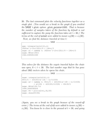
locity v0 = 196 − 196 e−9/2 = 64.607.... The distance fallen is
3 3
t
x1 (t) = 0 v1 (u) du
196 3
= 3 t + 3920 e− 20 t
9 − 3920
9 .
13720 3920 −9/2
After 30 seconds, it has fallen x1 (30) = 9 + 9 e =
1529.283... meters.

48. Taking m = 100, g = 9.8, k = 100 and v(0) = v0 , we find
49 833 196 −9/2
v2 (t) = + e−t − e .
5 15 3
This is the velocity with the time t starting the moment Wile
E. Coyote opens his chute (i.e., 30 seconds after jumping). The
distance fallen is
t
x2 (t) = 0 v2 (u) du + x1 (30)
49 833 −t
= 5 t − 15 e + 196 e−t e−9/2
3 + 71099
45 + 3332
9 e−9/2 .

49. Now let us solve this using SAGE .
SAGE
sage: RR = RealField(sci_not=0, prec=50, rnd=’RNDU’)
sage: t = var(’t’)
sage: v = function(’v’, t)
sage: m = 100; g = 98/10; k = 15
sage: de = lambda v: m*diff(v,t) + k*v - m*g
sage: desolve_laplace(de(v(t)),["t","v"],[0,0])
’196/3-196*%eˆ-(3*t/20)/3’
sage: soln1 = lambda t: 196/3-196*exp(-3*t/20)/3
sage: P1 = plot(soln1(t),0,30,plot_points=1000)
sage: RR(soln1(30))
64.607545559502
This solves for the velocity before the coyote’s chute is opened,
0 < t < 30. The last number is the velocity Wile E. Coyote is
traveling at the moment he opens his chute.
SAGE
sage: t = var(’t’)
sage: v = function(’v’, t)
sage: m = 100; g = 98/10; k = 100
sage: de = lambda v: m*diff(v,t) + k*v - m*g
sage: desolve_laplace(de(v(t)),["t","v"],[0,RR(soln1(30))])
’631931*%eˆ-t/11530+49/5’
sage: soln2 = lambda t: 49/5+(631931/11530)*exp(-(t-30))
+ soln1(30) - (631931/11530) - 49/5
sage: RR(soln2(30))
64.607545559502
sage: RR(soln1(30))
64.607545559502
sage: P2 = plot(soln2(t),30,50,plot_points=1000)
sage: show(P1+P2)
This solves for the velocity after the coyote’s chute is opened, t >

50. 30. The last command plots the velocity functions together as a
single plot. (You would see a break in the graph if you omitted
the SAGE ’s plot option ,plot_points=1000. That is because
the number of samples taken of the function by default is not
sufficient to capture the jump the function takes at t = 30.) The
terms at the end of soln2 were added to insure x2 (30) = x1 (30).
Next, we find the distance traveled at time t:
SAGE
age: integral(soln1(t),t)
3920*eˆ(-(3*t/20))/9 + 196*t/3
sage: x1 = lambda t: 3920*eˆ(-(3*t/20))/9 + 196*t/3
sage: RR(x1(30))
1964.8385851589
This solves for the distance the coyote traveled before the chute
was open, 0 < t < 30. The last number says that he has gone
about 1965 meters when he opens his chute.
SAGE
sage: integral(soln2(t),t)
49*t/5 - (631931*eˆ(30 - t)/11530)
sage: x2 = lambda t: 49*t/5 - (631931*eˆ(30 - t)/11530)
+ x1(30) + (631931/11530) - 49*30/5
sage: RR(x2(30.7))
1999.2895090436
sage: P4 = plot(x2(t),30,50)
sage: show(P3+P4)
(Again, you see a break in the graph because of the round-off
error.) The terms at the end of x2 were added to insure x2 (30) =
x1 (30). You know he is close to the ground at t = 30, and going

51. quite fast (about 65 m/s!). It makes sense that he will hit the
ground soon afterwards (with a large puff of smoke, if you’ve
seen the cartoons), even though his chute will have slowed him
down somewhat.
The graph of the velocity 0 < t < 50 is in Figure 1.11. Notice
how it drops at t = 30 when the chute is opened. The graph of
the distance fallen 0 < t < 50 is in Figure 1.12. Notice how it
slows down at t = 30 when the chute is opened.
Figure 1.11: Velocity of falling parachutist.
The time of impact is timpact = 30.7.... This was found numer-
ically by a “trial-and-error” method of solving x2 (t) = 2000.
The velocity of impact is v2 (timpact ) ≈ 37 m/s.
Exercise: Drop an object with mass 10 kgs from a height of
2000 m. Suppose the force due to air resistence is given by
Fres = −10v. Find the velocity after 10 seconds using SAGE .
Plot this velocity function for 0 < t < 10.

52. Figure 1.12: Distance fallen by a parachutist.
1.7 Application to mixing problems
Suppose that we have two chemical substances where one is
soluable in the other, such as salt and water. Suppose that we
have a tank containing a mixture of these substances, and the
mixture of them is poured in and the resulting “well-mixed”
solution pours out through a value at the bottom. (The term
“well-mixed” is used to indicate that the fluid being poured in
is assumed to instantly dissolve into a homogeneous mixture the
moment it goes into the tank.) The crude picture looks like this:
Assume for concreteness that the chemical substances are salt
and water. Let
• A(t) denote the amount of salt at time t,
• FlowRateIn = the rate at which the solution pours into the
tank,

53. Figure 1.13: Solution pours into a tank, mixes with another type of solution.
and then pours out.
• FlowRateOut = the rate at which the mixture pours out of
the tank,
• Cin = “concentration in” = the concentration of salt in the
solution being poured into the tank,
• Cout = “concentration out” = the concentration of salt in
the solution being poured out of the tank,
• Rin = rate at which the salt is being poured into the tank
= (FlowRateIn)(Cin ),
• Rout = rate at which the salt is being poured out of the
tank = (FlowRateOut)(Cout ).
Remark 1.7.1. Some things to make note of:

54. • If FlowRateIn = FlowRateOut then the “water level” of the
tank stays the same.
• We can determine Cout as a function of other quantities:
A(t)
Cout = ,
T (t)
where T (t) denotes the volume of solution in the tank at
time t.
• The rate of change of the amount of salt in the tank, A′ (t),
more properly could be called the “net rate of change”. If
you think if it this way then you see A′ (t) = Rin − Rout .
Now the differential equation for the amount of salt arises from
the above equations:
A(t)
A′ (t) = (FlowRateIn)Cin − (FlowRateOut) .
T (t)
Example 1.7.1. Consider a tank with 200 liters of salt-water
solution, 30 grams of which is salt. Pouring into the tank is a
brine solution at a rate of 4 liters/minute and with a concentra-
tion of 1 grams per liter. The “well-mixed” solution pours out
at a rate of 5 liters/minute. Find the amount at time t.
We know
A(t) A(t)
A′ (t) = (FlowRateIn)Cin −(FlowRateOut) = 4−5 , A(0) = 30.
T (t) 200 − t
Writing this in the standard form A′ + pA = q, we have
µ(t)q(t) dt + C
A(t) = ,
µ(t)

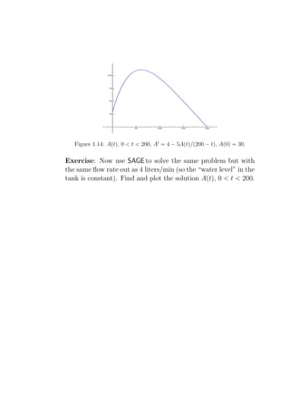
55. 1
where µ = e p(t) dt = e−5 200−t dt = (200 − t)−5 is the “integrating
factor”. This gives A(t) = 200 − t + C · (200 − t)5 , where the
initial condition implies C = −170 · 200−5 .
Here is one way to do this using SAGE :
SAGE
sage: t = var(’t’)
sage: A = function(’A’, t)
sage: de = lambda A: diff(A,t) + (5/(200-t))*A - 4
sage: desolve(de(A(t)),[A,t])
’(%c-1/(t-200)ˆ4)*(t-200)ˆ5’
This is the form of the general solution. (SAGE uses Maxima
and %c is Maxima’s notation for an arbitrary constant.) Let us
now solve this general solution for c, using the initial conditions.
SAGE
sage: c = var(’c’)
sage: solnA = lambda t: (c - 1/(t-200)ˆ4)*(t-200)ˆ5
sage: solnA(t)
(c - (1/(t - 200)ˆ4))*(t - 200)ˆ5
sage: solnA(0)
-320000000000*(c - 1/1600000000)
sage: solve([solnA(0) == 30],c)
[c == 17/32000000000]
sage: c = 17/32000000000
sage: solnA(t)
(17/32000000000 - (1/(t - 200)ˆ4))*(t - 200)ˆ5
sage: P = plot(solnA(t),0,200)
sage: show(P)

56. Figure 1.14: A(t), 0 < t < 200, A′ = 4 − 5A(t)/(200 − t), A(0) = 30.
Exercise: Now use SAGE to solve the same problem but with
the same flow rate out as 4 liters/min (so the “water level” in the
tank is constant). Find and plot the solution A(t), 0 < t < 200.

57. Chapter 2
Second order differential
equations
49

58. 2.1 Linear differential equations
We want to describe the form a solution to a linear ODE can
take. Before doing this, we introduce two pieces of terminology.
• Suppose f1 (t), f2 (t), . . . , fn (t) are given functions. A lin-
ear combination of these functions is another fucntion of
the form
c1 f1 (t) + c2 f2 (t) + . . . , +cn fn (t),
for some constants c1 , ..., cn . For example, 3 cos(t)−2 sin(t)
is a linear combination of cos(t), sin(t).
• A linear ODE of the form
y (n) + b1 (t)y (n−1) + ... + bn−1 (t)y ′ + bn (t)y = f (t), (2.1)
is called homogeneous if f (t) = 0 (i.e., f is the 0 function)
and otherwise it is called non-homogeneous.
The following result describes the general solution to a linear
ODE.
Theorem 2.1.1. Consider a linear ODE having of the form
(2.1), for some given continuous functions b1 (t), . . . , bn (t), and
f (t). Then the following hold.
• There are n functions y1 (t), . . . , yn (t) (called fundamen-
tal solutions), each satisfying the homogeneous ODE
y (n) + b1 (t)y (n−1) + ... + bn−1 (t)y ′ + bn (t)y = 0, 1 ≤ i ≤ n,
(2.2)

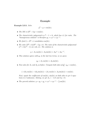
59. such that every solution to (2.2) is a linear combination of
these functions y1 , . . . , yn .
• Suppose you know a solution yp (t) (a particular solution)
to (2.1). Then every solution y = y(t) (the general solu-
tion) to the DE (2.1) has the form
y(t) = yh (t) + yp (t), (2.3)
where yh (the “homogeneous part” of the general solution)
is a linear combination
yh (t) = c1 y1 (t) + y2 (t) + ... + cn yn (t),
for some constants ci , 1 ≤ i ≤ n.
• Conversely, every function of the form (2.3), for any con-
stants ci for 1 ≤ i ≤ n, is a solution to (2.1).
Example 2.1.1. Recall the example in the introduction where
we looked for functions solving x′ + x = 1 by “guessing”. The
function xp (t) = 1 is a particular solution to x′ + x = 1. The
function x1 (t) = e−t is a fundamental solution to x′ + x = 0.
The general solution is therefore x(t) = 1 + c1 e−t , for a constant
c1 .
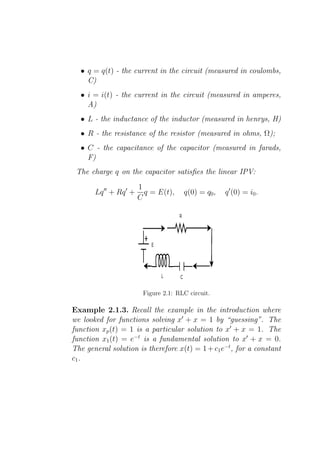
Example 2.1.2. The charge on the capacitor of an RLC elec-
trical circuit is modeled by a 2-nd order linear DE [C-linear].
Series RLC Circuit notations:
• E = E(t) - the voltage of the power source (a battery or
other “electromotive force”, measured in volts, V)

60. • q = q(t) - the current in the circuit (measured in coulombs,
C)
• i = i(t) - the current in the circuit (measured in amperes,
A)
• L - the inductance of the inductor (measured in henrys, H)
• R - the resistance of the resistor (measured in ohms, Ω);
• C - the capacitance of the capacitor (measured in farads,
F)
The charge q on the capacitor satisfies the linear IPV:
1
Lq ′′ + Rq ′ + q = E(t), q(0) = q0 , q ′ (0) = i0 .
C
Figure 2.1: RLC circuit.
Example 2.1.3. Recall the example in the introduction where
we looked for functions solving x′ + x = 1 by “guessing”. The
function xp (t) = 1 is a particular solution to x′ + x = 1. The
function x1 (t) = e−t is a fundamental solution to x′ + x = 0.
The general solution is therefore x(t) = 1 + c1 e−t , for a constant
c1 .

61. Example 2.1.4. The displacement from equilibrium of a mass
attached to a spring is modeled by a 2-nd order linear DE [O-ivp].
SSpring-mass notations:
• f (t) - the external force acting on the spring (if any)
• x = x(t) - the displacement from equilibrium of a mass
attached to a spring
• m - the mass
• b - the damping constant (if, say, the spring is immersed in
a fluid)
• k - the spring constant.
The displacement x satisfies the linear IPV:
mx′′ + bx′ + kx = f (t), x(0) = x0 , x′ (0) = v0 .
Figure 2.2: spring-mass model.

62. Notice that each general solution to an n-th order ODE has
n “degrees of freedom” (the arbitrary constants ci ). According
to this theorem, to find the general solution of a linear ODE,
we need only find a particular solution yp and n fundamental
solutions y1 (t), . . . , yn (t).
Example 2.1.5. Let us try to solve
x′ + x = 1, x(0) = c,
where c = 1, c = 2, and c = 3. (Three different IVP’s, three
different solutions, find each one.)
The first problem, x′ + x = 1 and x(0) = 1, is easy. The
solutions to the DE x′ + x = 1 which we “guessed at” in the
previous example, x(t) = 1, satisfies this.
The second problem, x′ + x = 1 and x(0) = 2, is not so simple.
To solve this (and the third problem), we really need to know
what the form is of the “general solution”.
According to the theorem above, the general solution x has the
form x = xp + xh . In this case, xp (t) = 1 and xh (t) = c1 x1 (t) =
c1 e−t , by an earlier example. Therefore, every solution to the
DE above is of the form x(t) = 1 + c1 e−t , for some constant c1 .
We use the initial condition to solve for c1 :
• x(0) = 1: 1 = x(0) = 1 + c1 e0 = 1 + c1 so c1 = 0 and
x(t) = 1.
• x(0) = 2: 2 = x(0) = 1 + c1 e0 = 1 + c1 so c1 = 1 and
x(t) = 1 + e−t .
• x(0) = 3: 3 = x(0) = 1 + c1 e0 = 1 + c1 so c1 = 2 and
x(t) = 1 + 2e−t .

63. Here is one way to use SAGE to solve for c1 . (Of course, you
can do this yourself, but this shows you the SAGE syntax for
solving equations. Type solve? in SAGE to get more details.)
We use SAGE to solve the last IVP discussed above and then to
plot the solution.
SAGE
sage: t = var(’t’)
sage: c1 = var(’c1’)
sage: solnx = lambda t: 1+c1*exp(-t)
sage: solnx(0)
c1 + 1
sage: solve([solnx(0) == 3],c1)
[c1 == 2]
sage: c_1 = solve([solnx(0) == 3],c1)[0].rhs()
sage: c_1
2
sage: solnx1 = lambda t: 1+c*exp(-t)
sage: plot(solnx1(t),0,2)
Graphics object consisting of 1 graphics primitive
sage: P = plot(solnx1(t),0,2)
sage: show(P)
sage: P = plot(solnx1(t),0,5)
sage: show(P)
This plot is shown below.

64. Figure 2.3: Solution to IVP x′ + x = 1, x(0) = 3.
Exercise: Use SAGE to solve and plot the solution to x′ + x = 1
and x(0) = 2.

65. 2.2 Linear differential equations, continued
To better describe the form a solution to a linear ODE can
take, we need to better understand the nature of fundamental
solutions and particular solutions.
Recall that the general solution to
y (n) + b1 (t)y (n−1) + ... + bn−1 (t)y ′ + bn (t)y = f (t),
has the form y = yp + yh , where yh is a linear combination of
fundamental solutions. For example, the general solution to the
spring-mass equation
x′′ + x = 1
has the form x = x(t) = 1 + c1 cos(t) + c2 sin(t) for the displace-
ment from the equilibrium position. Suppose we are also given n
initial conditions y(x0 ) = a0 , y ′ (x0 ) = a1 , . . . , y (n−1) (x0 ) = an−1 .
For example, we could impose the initial position and initial
velocity on the mass: x(0) = x0 and x′ (0) = v0 . Of course,
no matter what x0 and v0 are are given, we want to be able to
solve for the coefficients c1 , c2 in x(t) = 1 + c1 cos(t) + c2 sin(t)
to obtain a unique solution. More generally, we want to be able
to solve an n-th order IVP and obtain a unique solution. A few
questions arise.
• How do we know this can be done?
• How do we know that there isn’t a linear combination of
fundamental solutions which isn’t 0 (i.e., the zero function)?
The complete answer actually involves methods from linear
algebra which go beyond this course. The basic idea though

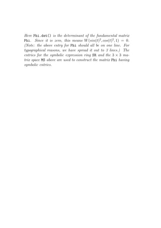
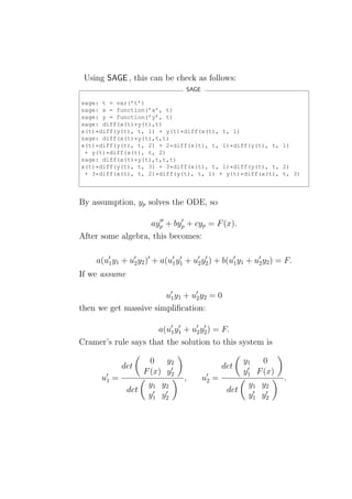
66. is not hard to understand and it involves what is called “the
Wronskian1 ” [W-linear]. We’ll have to explain what this means
first. If f1 (t), f2 (t), . . . , fn (t) are given n-times differentiable
functions then their fundamental matrix is the matrix
 
f1 (t) f2 (t) . . . fn (t)
′ ′ ′
 f1 (t) f2 (t) . . . fn (t) 
Φ = Φ(f1 , ..., fn ) =  . . . .
 
 .
. .
. .
. 
(n−1) (n−1) (n−1)
f1 (t) f2 (t) . . . fn (t)
The determinant of the fundamental matrix is called the Wron-
skian, denoted W (f1 , ..., fn ). The Wronskian actually helps us
answer both questions above simultaneously.
Example 2.2.1. Take f1 (t) = sin2 (t), f2 (t) = cos2 (t), and
f3 (t) = 1. SAGE allows us to easily compute the Wronskian:
SAGE
sage: SR = SymbolicExpressionRing()
sage: MS = MatrixSpace(SR,3,3)
sage: Phi = MS([[sin(t)ˆ2,cos(t)ˆ2,1],
[diff(sin(t)ˆ2,t),diff(cos(t)ˆ2,t),0],
[diff(sin(t)ˆ2,t,t),diff(cos(t)ˆ2,t,t),0]])
sage: Phi
[ sin(t)ˆ2 cos(t)ˆ2 1]
[ 2*cos(t)*sin(t) -2*cos(t)*sin(t) 0]
[2*cos(t)ˆ2 - 2*sin(t)ˆ2 2*sin(t)ˆ2 - 2*cos(t)ˆ2 0]
sage: Phi.det()
0
1
Josef Wronski was a Polish-born French mathemtician who worked in many different
areas of applied mathematics and mechanical engineering [Wr-linear].

67. Here Phi.det() is the determinant of the fundamental matrix
Phi. Since it is zero, this means W (sin(t)2 , cos(t)2 , 1) = 0.
(Note: the above entry for Phi should all be on one line. For
typographical reasons, we have spread it out to 3 lines.) The
entries for the symbolic expression ring SR and the 3 × 3 ma-
trix space MS above are used to construct the matrix Phi having
symbolic entries.

68. We try one more example:
SAGE
sage: SR = SymbolicExpressionRing()
sage: MS = MatrixSpace(SR,2,2)
sage: Phi = MS([[sin(t)ˆ2,cos(t)ˆ2],
[diff(sin(t)ˆ2,t),diff(cos(t)ˆ2,t)]])
sage: Phi
[ sin(t)ˆ2 cos(t)ˆ2]
[ 2*cos(t)*sin(t) -2*cos(t)*sin(t)]
sage: Phi.det()
-2*cos(t)*sin(t)ˆ3 - 2*cos(t)ˆ3*sin(t)
This means W (sin(t)2 , cos(t)2 ) = −2 cos(t) sin(t)3 −2 cos(t)3 sin(t),
which is non-zero.
If there are constants c1 , ..., cn , not all zero, for which
c1 f1 (t) + c2 f2 (t) · · · + cn fn (t) = 0, for all t, (2.4)
then the functions fi (1 ≤ i ≤ n) are called linearly depen-
dent. If the functions fi (1 ≤ i ≤ n) are not linearly dependent
then they are called linearly independent (this definition is
frequently seen for linearly independent vectors [L-linear] but
holds for functions as well). This condition (2.4) can be inter-
preted geometrically as follows. Just as c1 x + c2 y = 0 is a line
through the origin in the plane and c1 x + c2 y + c3 z = 0 is a plane
containing the origin in 3-space, the equation
c1 x1 + c2 x2 · · · + cn xn = 0,
is a “hyperplane” containing the origin in n-space with coordi-
nates (x1 , ..., xn ). This condition (2.4) says geometrically that

69. the graph of the space curve r(t) = (f1 (t), . . . , fn (t)) lies en-
tirely in this hyperplane. If you pick n functions “at random”
then they are “probably” linearly independent, because “ran-
dom” space curves don’t lie in a hyperplane. But certainly not
all collections of functions are linearly independent.
Example 2.2.2. Consider just the two functions f1 (t) = sin2 (t),
f2 (t) = cos2 (t). We know from the SAGE computation in the
example above that these functions are linearly independent.
SAGE
sage: P = parametric_plot((sin(t)ˆ2,cos(t)ˆ2),0,5)
sage: show(P)
The SAGE plot of this space curve r(t) = (sin(t)2 , cos(t)2 ) is
given below. It is obviously not contained in a line through the
origin, therefore making it geometrically clear that these func-
tions are linearly independent.
The following two results answer the above questions.
Theorem 2.2.1. (Wronskian test) If f1 (t), f2 (t), . . . , fn (t)
are given n-times differentiable functions with a non-zero Wron-
skian then they are linearly independent.
As a consequence of this theorem, and the SAGE computation
in the example above, f1 (t) = sin2 (t), f2 (t) = cos2 (t), are lin-
early independent.
Theorem 2.2.2. Given any homogeneous n-th linear ODE
y (n) + b1 (t)y (n−1) + ... + bn−1 (t)y ′ + bn (t)y = 0,
with differentiable coefficients, there always exists n solutions
y1 (t), ..., yn (t) which have a non-zero Wronskian.

70. Figure 2.4: Parametric plot of (sin(t)2 , cos(t)2 ).
The functions y1 (t), ..., yn (t) in the above theorem are called
fundamental solutions.
We shall not prove either of these theorems here. Please see
[BD-intro] for further details.
Exercise: Use SAGE to compute the Wronskian of
(a) f1 (t) = sin(t), f2 (t) = cos(t),
(b) f1 (t) = 1, f2 (t) = t, f3 (t) = t2 , f4 (t) = t3 .
Check that
(a) y1 (t) = sin(t), y2 (t) = cos(t) are fundamental solutions for
′′
y + y = 0,
(d) y1 (t) = 1, y2 (t) = t, y3 (t) = t2 , y4 (t) = t3 are fundamental
solutions for y (4) = y ′′′′ = 0.

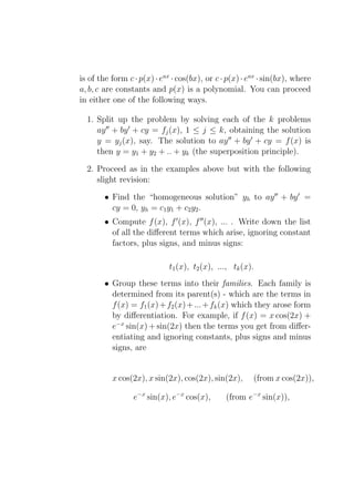
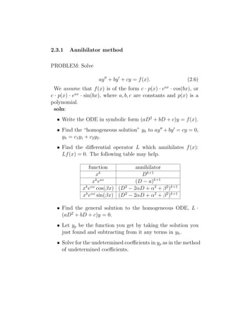
71. 2.3 Undetermined coefficients method
The method of undetermined coefficients [U-uc] can be used to
solve the following type of problem.
PROBLEM: Solve
ay ′′ + by ′ + cy = f (x), (2.5)
where a = 0, b and c are constants and x is the independent
variable. (Even the case a = 0 can be handled similarly, though
some of the discussion below might need to be slightly modified.)
Where we must assume that f (x) is of a special form.
More-or-less equivalent is the method of annihilating operators
[A-uc] (they solve the same class of DEs), but that method will
be discussed separately.
For the moment, let us assume f (x) has the form a1 · p(x) ·
ea2 x · cos(a3 x), or a1 · p(x) · ea2 x · sin(a3 x), where a1 , a2 , a3 are
constants and p(x) is a polynomial.
Solution:
• Find the “homogeneous solution” yh to ay ′′ + by ′ + cy =
0, yh = c1 y1 + c2 y2 . Here y1 and y2 are determined as
follows: let r1 and r2 denote the roots of the characteristic
polynomial aD2 + bD + c = 0.
– r1 = r2 real: set y1 = er1 x , y2 = er2 x .
– r1 = r2 real: if r = r1 = r2 then set y1 = erx , y2 = xerx .
– r1 , r2 complex: if r1 = α + iβ, r2 = α − iβ, where α and
β are real, then set y1 = eαx cos(βx), y2 = eαx sin(βx).

72. • Compute f (x), f ′ (x), f ′′ (x), ... . Write down the list of
all the different terms which arise (via the product rule),
ignoring constant factors, plus signs, and minus signs:
t1 (x), t2 (x), ..., tk (x).
If any one of these agrees with y1 or y2 then multiply them
all by x. (If, after this, any of them still agrees with y1 or
y2 then multiply them all again by x.)
• Let yp be a linear combination of these functions (your
“guess”):
yp = A1 t1 (x) + ... + Ak tk (x).
This is called the general form of the particular solu-
tion. The Ai ’s are called undetermined coefficients.
• Plug yp into (2.5) and solve for A1 , ..., Ak .
• Let y = yh + yp = yp + c1 y1 + c2 y2 . This is the general
solution to (2.5). If there are any initial conditions for
(2.5), solve for then c1 , c2 now.
Diagramatically:
Factor characteristic polynomial
↓
Compute yh

73. ↓
Compute the general form of the particular, yp
↓
Compute the undetermined coefficients
↓
Answer: y = yh + yp .

74. Examples
Example 2.3.1. Solve
y ′′ − y = cos(2x).
• The characteristic polynomial is r2 − 1 = 0, which has ±1 for roots. The
“homogeneous solution” is therefore yh = c1 ex + c2 e−x .
• We compute f (x) = cos(2x), f ′ (x) = −2 sin(2x), f ′′ (x) = −4 cos(2x), ... .
They are all linear combinations of
f1 (x) = cos(2x), f2 (x) = sin(2x).
None of these agrees with y1 = ex or y2 = e−x , so we do not multiply by x.
• Let yp be a linear combination of these functions:
yp = A1 cos(2x) + A2 sin(2x).
′′
• You can compute both sides of yp − yp = cos(2x):
(−4A1 cos(2x) − 4A2 sin(2x)) − (A1 cos(2x) + A2 sin(2x)) = cos(2x).
Equating the coefficients of cos(2x), sin(2x) on both sides gives 2 equations
in 2 unknowns: −5A1 = 1 and −5A2 = 0. Solving, we get A1 = −1/5 and
A2 = 0.
1
• The general solution: y = yh + yp = c1 ex + c2 e−x − 5 cos(2x).
Example 2.3.2. Solve
y ′′ − y = x cos(2x).
• The characteristic polynomial is r2 − 1 = 0, which has ±1 for roots. The
“homogeneous solution” is therefore yh = c1 ex + c2 e−x .
• We compute f (x) = x cos(2x), f ′ (x) = cos(2x)−2x sin(2x), f ′′ (x) = −2 sin(2x)−
2 sin(2x) − 2x cos(2x), ... . They are all linear combinations of
f1 (x) = cos(2x), f2 (x) = sin(2x), f3 (x) = x cos(2x), .f4 (x) = x sin(2x).
None of these agrees with y1 = ex or y2 = e−x , so we do not multiply by x.

75. • Let yp be a linear combination of these functions:
yp = A1 cos(2x) + A2 sin(2x) + A3 x cos(2x) + A4 x sin(2x).
′′
• In principle, you can compute both sides of yp − yp = x cos(2x) and solve for
the Ai ’s. (Equate coefficients of x cos(2x) on both sides, equate coefficients
of cos(2x) on both sides, equate coefficients of x sin(2x) on both sides, and
equate coefficients of sin(2x) on both sides. This gives 4 equations in 4
unknowns, which can be solved.) You will not be asked to solve for the Ai ’s
for a problem this hard.
Example 2.3.3. Solve
y ′′ + 4y = x cos(2x).
• The characteristic polynomial is r2 + 4 = 0, which has ±2i for roots. The
“homogeneous solution” is therefore yh = c1 cos(2x) + c2 sin(2x).
• We compute f (x) = x cos(2x), f ′ (x) = cos(2x)−2x sin(2x), f ′′ (x) = −2 sin(2x)−
2 sin(2x) − 2x cos(2x), ... . They are all linear combinations of
f1 (x) = cos(2x), f2 (x) = sin(2x), f3 (x) = x cos(2x), .f4 (x) = x sin(2x).
Two of these agree with y1 = cos(2x) or y2 = sin(2x), so we do multiply by
x:
f1 (x) = x cos(2x), f2 (x) = x sin(2x), f3 (x) = x2 cos(2x), .f4 (x) = x2 sin(2x).
• Let yp be a linear combination of these functions:
yp = A1 x cos(2x) + A2 x sin(2x) + A3 x2 cos(2x) + A4 x2 sin(2x).
′′
• In principle, you can compute both sides of yp + 4yp = x cos(2x) and solve
for the Ai ’s. You will not be asked to solve for the Ai ’s for a problem this
hard.
More generally, suppose that you want to solve ay ′′ +by ′ +cy =
f (x), where f (x) is a sum of functions of the above form. In
other words, f (x) = f1 (x) + f2 (x) + ... + fk (x), where each fj (x)

76. is of the form c · p(x) · eax · cos(bx), or c · p(x) · eax · sin(bx), where
a, b, c are constants and p(x) is a polynomial. You can proceed
in either one of the following ways.
1. Split up the problem by solving each of the k problems
ay ′′ + by ′ + cy = fj (x), 1 ≤ j ≤ k, obtaining the solution
y = yj (x), say. The solution to ay ′′ + by ′ + cy = f (x) is
then y = y1 + y2 + .. + yk (the superposition principle).
2. Proceed as in the examples above but with the following
slight revision:
• Find the “homogeneous solution” yh to ay ′′ + by ′ =
cy = 0, yh = c1 y1 + c2 y2 .
• Compute f (x), f ′ (x), f ′′ (x), ... . Write down the list
of all the different terms which arise, ignoring constant
factors, plus signs, and minus signs:
t1 (x), t2 (x), ..., tk (x).
• Group these terms into their families. Each family is
determined from its parent(s) - which are the terms in
f (x) = f1 (x) + f2 (x) + ... + fk (x) which they arose form
by differentiation. For example, if f (x) = x cos(2x) +
e−x sin(x) + sin(2x) then the terms you get from differ-
entiating and ignoring constants, plus signs and minus
signs, are
x cos(2x), x sin(2x), cos(2x), sin(2x), (from x cos(2x)),
e−x sin(x), e−x cos(x), (from e−x sin(x)),

77. and
sin(2x), cos(2x), (from sin(2x)).
The first group absorbes the last group, since you can
only count the different terms. Therefore, there are
only two families in this example: {x cos(2x), x sin(2x), cos(2x), sin(2x)}
is a “family” (with “parent” x cos(2x) and the other
terms as its “children”) and {e−x sin(x), e−x cos(x)} is
a “family” (with “parent” e−x sin(x) and the other term
as its “child”).
If any one of these terms agrees with y1 or y2 then
multiply the entire family by x. In other words, if any
child or parent is “bad” then the entire family is “bad”.
(If, after this, any of them still agrees with y1 or y2 then
multiply them all again by x.)
• Let yp be a linear combination of these functions (your
“guess”):
yp = A1 t1 (x) + ... + Ak tk (x).
This is called the general form of the particular
solution. The Ai ’s are called undetermined coeffi-
cients.
• Plug yp into (2.5) and solve for A1 , ..., Ak .
• Let y = yh + yp = yp + c1 y1 + c2 y2 . This is the general
solution to (2.5). If there are any initial conditions for
(2.5), solve for then c1 , c2 last - after the undetermined
coefficients.
Example 2.3.4. Solve
y ′′′ − y ′′ − y ′ + y = 12xex .

78. We use SAGE for this.
SAGE
sage: x = var("x")
sage: y = function("y",x)
sage: R.<D> = PolynomialRing(QQ, "D")
sage: f = Dˆ3 - Dˆ2 - D + 1
sage: f.factor()
(D + 1) * (D - 1)ˆ2
sage: f.roots()
[(-1, 1), (1, 2)]
So the roots of the characteristic polynomial are 1, 1, −1, which
means that the homogeneous part of the solution is
yh = c1 ex + c2 xex + c3 e−x .
SAGE
sage: de = lambda y: diff(y,x,3) - diff(y,x,2) - diff(y,x,1) + y
sage: c1 = var("c1"); c2 = var("c2"); c3 = var("c3")
sage: yh = c1*eˆx + c2*x*eˆx + c3*eˆ(-x)
sage: de(yh)
0
sage: de(xˆ3*eˆx-(3/2)*xˆ2*eˆx)
12*x*eˆx
This just confirmed that yh solves y ′′′ − y ′′ − y ′ + 1 = 0. Using
the derivatives of F (x) = 12xex , we generate the general form
of the particular:
SAGE
sage: F = 12*x*eˆx

79. sage: diff(F,x,1); diff(F,x,2); diff(F,x,3)
12*x*eˆx + 12*eˆx
12*x*eˆx + 24*eˆx
12*x*eˆx + 36*eˆx
sage: A1 = var("A1"); A2 = var("A2")
sage: yp = A1*xˆ2*eˆx + A2*xˆ3*eˆx
Now plug this into the DE and compare coefficients of like terms
to solve for the undertermined coefficients:
SAGE
sage: de(yp)
12*x*eˆx*A2 + 6*eˆx*A2 + 4*eˆx*A1
sage: solve([12*A2 == 12, 6*A2+4*A1 == 0],A1,A2)
[[A1 == -3/2, A2 == 1]]
Finally, lets check if this is correct:
SAGE
sage: y = yh + (-3/2)*xˆ2*eˆx + (1)*xˆ3*eˆx
sage: de(y)
12*x*eˆx
Exercise: Using SAGE , solve
y ′′′ − y ′′ + y ′ − y = 12xex .
(Hint: You may need to replace sage: R.<D> = PolynomialRing(QQ, "D")
by sage: R.<D> = PolynomialRing(CC, "D").)

80. 2.3.1 Annihilator method
PROBLEM: Solve
ay ′′ + by ′ + cy = f (x). (2.6)
We assume that f (x) is of the form c · p(x) · eax · cos(bx), or
c · p(x) · eax · sin(bx), where a, b, c are constants and p(x) is a
polynomial.
soln:
• Write the ODE in symbolic form (aD2 + bD + c)y = f (x).
• Find the “homogeneous solution” yh to ay ′′ + by ′ = cy = 0,
yh = c 1 y1 + c 2 y2 .
• Find the differential operator L which annihilates f (x):
Lf (x) = 0. The following table may help.
function annihilator
k
x Dk+1
xk eax (D − a)k+1
xk eαx cos(βx) (D2 − 2αD + α2 + β 2 )k+1
xk eαx sin(βx) (D2 − 2αD + α2 + β 2 )k+1
• Find the general solution to the homogeneous ODE, L ·
(aD2 + bD + c)y = 0.
• Let yp be the function you get by taking the solution you
just found and subtracting from it any terms in yh .
• Solve for the undetermined coefficients in yp as in the method
of undetermined coefficients.

81. Example
Example 2.3.5. Solve
y ′′ − y = cos(2x).
• The DE is (D2 − 1)y = cos(2x).
• The characteristic polynomial is r2 − 1 = 0, which has ±1 for roots. The
“homogeneous solution” is therefore yh = c1 ex + c2 e−x .
• We find L = D2 + 4 annihilates cos(2x).
• We solve (D2 + 4)(D2 − 1)y = 0. The roots of the characteristic polynomial
(r2 + 4)(r2 − 1) are ±2i, ±1. The solution is
y = A1 cos(2x) + A2 sin(2x) + A3 ex + A4 e−x .
• This solution agrees with yh in the last two terms, so we guess
yp = A1 cos(2x) + A2 sin(2x).
′′
• Now solve for A1 and A2 as before: Compute both sides of yp −yp = cos(2x),
(−4A1 cos(2x) − 4A2 sin(2x)) − (A1 cos(2x) + A2 sin(2x)) = cos(2x).
Next, equate the coefficients of cos(2x), sin(2x) on both sides to get 2 equa-
tions in 2 unknowns. Solving, we get A1 = −1/5 and A2 = 0.
• The general solution: y = yh + yp = c1 ex + c2 e−x − 1 cos(2x).
5

82. 2.4 Variation of parameters
Consider an ordinary constant coefficient non-homogeneous 2nd
order linear differential equation,
ay ′′ + by ′ + cy = F (x)
where F (x) is a given function and a, b, and c are constants. (For
the method below, a, b, and c may be allowed to depend on the
independent variable x as well.) Let y1 (x), y2 (x) be fundamental
solutions of the corresponding homogeneous equation
ay ′′ + by ′ + cy = 0.
The method of variation of parameters is originally attributed
to Joseph Louis Lagrange (1736-1813) [L-var]. It starts by as-
suming that there is a particular solution in the form
yp (x) = u1 (x)y1 (x) + u2 (x)y2 (x),
where u1 (x), u2 (x) are unknown functions [V-var].
In general, the product rule gives
(f g)′ = f ′ g + f g ′ ,
(f g)′′ = f ′′ g + 2f ′ g ′ + f g ′′ ,
(f g)′′′ = f ′′′ g + 3f ′′ g ′ + 3f ′ g ′′ + f g ′′′ ,
and so on, following Pascal’s triangle,
1
1 1

83. 1 2 1
1 3 3 1,
and so on.

84. Using SAGE , this can be check as follows:
SAGE
sage: t = var(’t’)
sage: x = function(’x’, t)
sage: y = function(’y’, t)
sage: diff(x(t)*y(t),t)
x(t)*diff(y(t), t, 1) + y(t)*diff(x(t), t, 1)
sage: diff(x(t)*y(t),t,t)
x(t)*diff(y(t), t, 2) + 2*diff(x(t), t, 1)*diff(y(t), t, 1)
+ y(t)*diff(x(t), t, 2)
sage: diff(x(t)*y(t),t,t,t)
x(t)*diff(y(t), t, 3) + 3*diff(x(t), t, 1)*diff(y(t), t, 2)
+ 3*diff(x(t), t, 2)*diff(y(t), t, 1) + y(t)*diff(x(t), t, 3)
By assumption, yp solves the ODE, so
′′ ′
ayp + byp + cyp = F (x).
After some algebra, this becomes:
a(u′1 y1 + u′2 y2 )′ + a(u′1 y1 + u′2 y2 ) + b(u′1 y1 + u′2 y2 ) = F.
′ ′
If we assume
u′1 y1 + u′2 y2 = 0
then we get massive simplification:
a(u′1 y1 + u2 y2 ) = F.
′ ′ ′
Cramer’s rule says that the solution to this system is
0 y2 y1 0
det ′ det ′
F (x) y2 y1 F (x)
u′1 = , u′2 = .
y1 y2 y1 y2
det ′ ′ det ′ ′
y1 y2 y1 y2

85. Note that the Wronskian of the fundamental solutions W (y1 , y2 )
is in the denominator.
Solve these for u1 and u2 by integration and then plug them
back into yp to get your particular solution.
Example 2.4.1. Solve
y ′′ + y = tan(x).
soln: The functions y1 = cos(x) and y2 = sin(x) are funda-
mental solutions with Wronskian W (cos(x), sin(x)) = 1. The
Cramer’s rule formulas above become:
0 sin(x) cos(x) 0
det det
tan(x) cos(x) − sin(x) tan(x)
u′1 = , u′2 = .
1 1
Therefore,
sin2 (x)
u′1
=− , u′2 = sin(x).
cos(x)
Therefore, using methods from integral calculus, u1 = − ln | tan(x)+
sec(x)| + sin(x) and u2 = − cos(x). Using SAGE , this can be
check as follows:
SAGE
sage: integral(-sin(t)ˆ2/cos(t),t)
-log(sin(t) + 1)/2 + log(sin(t) - 1)/2 + sin(t)
sage: integral(cos(t)-sec(t),t)
sin(t) - log(tan(t) + sec(t))
sage: integral(sin(t),t)
-cos(t)
As you can see, there are other forms the answer can take. The
particular solution is

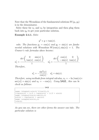
86. yp = (− ln | tan(x) + sec(x)| + sin(x)) cos(x) + (− cos(x)) sin(x).
The homogeneous (or complementary) part of the solution is
yh = c1 cos(x) + c2 sin(x),
so the general solution is
y = yh + yp = c1 cos(x) + c2 sin(x)
+(− ln | tan(x) + sec(x)| + sin(x)) cos(x) + (− cos(x)) sin(x).
Using SAGE , this can be carried out as follows:
SAGE
sage: SR = SymbolicExpressionRing()
sage: MS = MatrixSpace(SR, 2, 2)
sage: W = MS([[cos(t),sin(t)],[diff(cos(t), t),diff(sin(t), t)]])
sage: W
[ cos(t) sin(t)]
[-sin(t) cos(t)]
sage: det(W)
sin(t)ˆ2 + cos(t)ˆ2
sage: U1 = MS([[0,sin(t)],[tan(t),diff(sin(t), t)]])
sage: U2 = MS([[cos(t),0],[diff(cos(t), t),tan(t)]])
sage: integral(det(U1)/det(W),t)
-log(sin(t) + 1)/2 + log(sin(t) - 1)/2 + sin(t)
sage: integral(det(U2)/det(W),t)
-cos(t)
Exercise: Use SAGE to solve y ′′ + y = cot(x).

87. 2.5 Applications of DEs: Spring problems
2.5.1 Part 1
Ut tensio, sic vis2 .
- Robert Hooke, 1678
One of the ways DEs arise is by means of modeling physical
phenomenon, such as spring equations. For these problems, con-
sider a spring suspended from a ceiling. We shall consider three
cases: (1) no mass is attached at the end of the spring, (2) a
mass is attached and the system is in the rest position, (3) a
mass is attached and the mass has been displaced fomr the rest
position.
Figure 2.5: A spring
at rest, without mass Figure 2.6: A spring Figure 2.7: A spring in
attached. at rest, with mass at- motion.
tached.
2
“As the extension, so the force.”

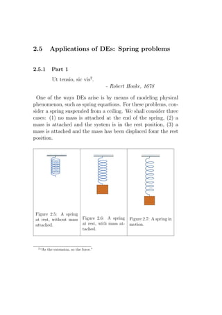
88. One can also align the springs left-to-right instead of top-to-
bottom, without changing the discussion below.
Notation: Consider the first two situations above: (a) a spring
at rest, without mass attached and (b) a spring at rest, with
mass attached. The distance the mass pulls the spring down is
sometimes called the “stretch”, and denoted s. (A formula for
s will be given later.)
Now place the mass in motion by imparting some initial ve-
locity (tapping it upwards with a hammer, say, and start your
timer). Consider the second two situations above: (a) a spring
at rest, with mass attached and (b) a spring in motion. The
difference between these two positions at time t is called the
displacement and is denoted x(t). Signs here will be choosen so
that down is positive.
Assume exactly three forces act:
1. the restoring force of the spring, Fspring ,
2. an external force (driving the ceiling up and down, but may
be 0), Fext ,
3. a damping force (imagining the spring immersed in oil or
that it is in fact a shock absorber on a car), Fdamp .
In other words, the total force is given by
Ftotal = Fspring + Fext + Fdamp .
Physics tells us that the following are approximately true:
1. (Hooke’s law [H-intro]): Fspring = −kx, for some “spring
constant” k > 0,

89. 2. Fext = F (t), for some (possibly zero) function F ,
3. Fdamp = −bv, for some “damping constant” b ≥ 0 (where v
denotes velocity),
4. (Newton’s 2nd law [N-mech]): Ftotal = ma (where a denotes
acceleration).
Putting this all together, we obtain mx′′ = ma = −kx + F (t) −
bv = −kx + F (t) − bx′ , or
mx′′ + bx′ + kx = F (t).
This is the spring equation. When b = F (t) = 0 this is also
called the equation for simple harmonic motion.
Consider again first two figures above: (a) a spring at rest,
without mass attached and (b) a spring at rest, with mass at-
tached. The mass in the second figure is at rest, so the gravita-
tional force on the mass, mg, is balanced by the restoring force
of the spring: mg = ks, where s is the stretch.In particular, the
spring constant can be computed from the stretch:
mg
k= s .
Example:
A spring at rest is suspended from the ceiling without mass. A
2 kg weight is then attached to this spring, stretching it 9.8 cm.
From a position 2/3 m above equilibrium the weight is give a
downward velocity of 5 m/s.
(a) Find the equation of motion.

90. (b) What is the amplitude and period of motion?
(c) At what time does the mass first cross equilibrium?
(d) At what time is the mass first exactly 1/2 m below equilib-
rium?
We shall solve this problem using SAGE below. Note m = 2,
b = F (t) = 0 (since no damping or external force is even
mentioned), and k = mg/s = 2 · 9.8/(0.098) = 200. There-
fore, the DE is 2x′′ + 200x = 0. This has general solution
x(t) = c1 cos(10t) + c2 sin(10t). The constants c1 and c2 can
be computed from the initial conditions x(0) = −2/3 (down is
positive, up is negative), x′ (0) = 5.
Using SAGE , the displacement can be computed as follows:
SAGE
sage: t = var(’t’)
sage: x = function(’x’, t)
sage: m = var(’m’)
sage: b = var(’b’)
sage: k = var(’k’)
sage: F = var(’F’)
sage: de = lambda y: m*diff(y,t,t) + b*diff(y,t) + k*y - F
sage: de(x(t))
-F + m*diff(x(t), t, 2) + b*diff(x(t), t, 1) + k*x(t)
sage: m = 2; b = 0; k = 2*9.8/(0.098); F = 0
sage: de(x(t))
2*diff(x(t), t, 2) + 200.000000000000*x(t)
sage: desolve(de(x(t)),[x,t])
’%k1*sin(10*t)+%k2*cos(10*t)’
sage: desolve_laplace(de(x(t)),["t","x"],[0,-2/3,5])
’sin(10*t)/2-2*cos(10*t)/3’
Now we write this in the more compact and useful form A sin(ωt+
φ) using the formulas

91. c1 cos(ωt) + c2 sin(ωt) = A sin(ωt + φ),
−2/3
where A = c2 + c2 denotes the amplitude and φ = 2 arctan( 1/2+A ).
1 2
SAGE
sage: A = sqrt((-2/3)ˆ2+(1/2)ˆ2)
sage: A
5/6
sage: phi = 2*atan((-2/3)/(1/2 + A))
sage: phi
-2*atan(1/2)
sage: RR(phi)
-0.927295218001612
sage: sol = lambda t: sin(10*t)/2-2*cos(10*t)/3
sage: sol2 = lambda t: A*sin(10*t + phi)
sage: P = plot(sol(t),0,2)
sage: show(P)
This is displayed below3 .
3
You can also, if you want, type show(plot(sol2(t),0,2)) to check that these two
functions are indeed the same.

92. Figure 2.8: Plot of 2x′′ + 200x = 0, x(0) = −2/3, x′ (0) = 5, for 0 < t < 2.
Of course, the period is 2π/10 = π/5 ≈ 0.628.
To answer (c) and (d), we solve x(t) = 0 and x(t) = 1/2:
SAGE
sage: solve(A*sin(10*t + phi) == 0,t)
[t == atan(1/2)/5]
sage: RR(atan(1/2)/5)
0.0927295218001612
sage: solve(A*sin(10*t + phi) == 1/2,t)
[t == (asin(3/5) + 2*atan(1/2))/10]
sage: RR((asin(3/5) + 2*atan(1/2))/10)
0.157079632679490
In other words, x(0.0927...) ≈ 0, x(0.157...) ≈ 1/2.

93. Exercise: Use the problem above.
(a) At what time does the weight pass through the equilibrium
position heading down for the 2nd time?
(b) At what time is the weight exactly 5/12 m below equilibrium
and heading up?

94. 2.5.2 Part 2
Recall from part 1, the spring equation
mx′′ + bx′ + kx = F (t)
where x(t) denotes the displacement at time t.
Unless otherwise stated, we assume there is no external force:
F (t) = 0.
The roots of the characteristic polynomial mD2 + bD = k = 0
are
√
−b ± b2 − 4mk
.
2m
There are three cases:
(a) real distinct roots: in this case the discriminant b2 − 4mk
is positive, so b2 > 4mk. In other words, b is “large”. This
case is referred to as overdamped. In this case, the roots
are negative,
√ √
−b − b2 − 4mk −b + b2 − 4mk
r1 = < 0, and r1 = < 0,
2m 2m
so the solution x(t) = c1 er1 t + c2 er2 t is exponentially de-
creasing.
(b) real repeated roots: in this case the discriminant b2 − 4mk
√
is zero, so b = 4mk. This case is referred to as criti-
cally damped. This case is said to model new suspension
systems in cars [D-spr].

95. (c) Complex roots: in this case the discriminant b2 − 4mk is
negative, so b2 < 4mk. In other words, b is “small”. This
case is referred to as underdamped (or simple harmonic
when b = 0).
Example: An 8 lb weight stretches a spring 2 ft. Assume a
damping force numerically equal to 2 times the instantaneous
velocity acts. Find the displacement at time t, provided that it
is released from the equilibrium position with an upward velocity
of 3 ft/s. Find the equation of motion and classify the behaviour.
We know m = 8/32 = 1/4, b = 2, k = mg/s = 8/2 = 4,
x(0) = 0, and x′ (0) = −3. This means we must solve
1 ′′
x + 2x′ + 4x = 0, x(0) = 0, x′ (0) = −3.
4
The roots of the characteristic polynomial are −4 and −4 (so
we are in the repeated real roots case), so the general solution
is x(t) = c1 e−4t + c2 te−4t . The initial conditions imply c1 = 0,
c2 = −3, so
x(t) = −3te−4t .
Using SAGE , we can compute this as well:
SAGE
sage: t = var(‘‘t’’)
sage: x = function(‘‘x’’)
sage: de = lambda y: (1/4)*diff(y,t,t) + 2*diff(y,t) + 4*y
sage: de(x(t))
diff(x(t), t, 2)/4 + 2*diff(x(t), t, 1) + 4*x(t)
sage: desolve(de(x(t)),[x,t])
’(%k2*t+%k1)*%eˆ-(4*t)’
sage: desolve_laplace(de(x(t)),[‘‘t’’,’’x’’],[0,0,-3])

96. ’-3*t*%eˆ-(4*t)’
sage: f = lambda t : -3*t*eˆ(-4*t)
sage: P = plot(f,0,2)
sage: show(P)
The graph is shown below.
Figure 2.9: Plot of (1/4)x′′ +2x′ +4x = 0, x(0) = 0, x′ (0) = −3, for 0 < t < 2.
Example: An 2 kg weight is attached to a spring having spring
constant 10. Assume a damping force numerically equal to 4
times the instantaneous velocity acts. Find the displacement at
time t, provided that it is released from 1 m below equilibrium
with an upward velocity of 1 ft/s. Find the equation of motion
and classify the behaviour.
Using SAGE , we can compute this as well:
SAGE
sage: t = var(‘‘t’’)
sage: x = function(‘‘x’’)

97. sage: de = lambda y: 2*diff(y,t,t) + 4*diff(y,t) + 10*y
sage: desolve_laplace(de(x(t)),["t","x"],[0,1,1])
’%eˆ-t*(sin(2*t)+cos(2*t))’
sage: desolve_laplace(de(x(t)),["t","x"],[0,1,-1])
’%eˆ-t*cos(2*t)’
sage: sol = lambda t: eˆ(-t)*cos(2*t)
sage: P = plot(sol(t),0,2)
sage: show(P)
sage: P = plot(sol(t),0,4)
sage: show(P)
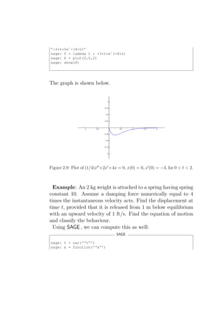
The graph is shown below.
Figure 2.10: Plot of 2x′′ + 4x′ + 10x = 0, x(0) = 1, x′ (0) = −1, for 0 < t < 4.

98. Exercise: Use the problem above. Use SAGE to find what time
the weight passes through the equilibrium position heading down
for the 2nd time.
Exercise: An 2 kg weight is attached to a spring having spring
constant 10. Assume a damping force numerically equal to 4
times the instantaneous velocity acts. Use SAGE to find the dis-
placement at time t, provided that it is released from 1 m below
equilibrium (with no initial velocity).
2.5.3 Part 3
If the frequency of the driving force of the spring matches the
frequency of the homogeneous part xh (t), in other words if
x′′ + ω 2 x = F0 cos(γt),
satisfies ω = γ then we say that the spring-mass system is in
(pure, mechanical) resonance.
Example: Solve
x′′ + ω 2 x = F0 cos(γt), x(0) = 0, x′ (0) = 0,
where ω = γ = 2 (ie, mechanical resonance). We use SAGE for
this:
SAGE
sage: t = var(’t’)
sage: x = function(’x’, t)
sage: (m,b,k,w,F0) = var("m,b,k,w,F0")
sage: de = lambda y: diff(y,t,t) + wˆ2*y - F0*cos(w*t)

99. sage: m = 1; b = 0; k = 4; F0 = 1; w = 2
sage: desolve(de(x(t)),[x,t])
’(2*t*sin(2*t)+cos(2*t))/8+%k1*sin(2*t)+%k2*cos(2*t)’
sage: desolve_laplace(de(x(t)),["t","x"],[0,0,0])
’t*sin(2*t)/4’
sage: soln = lambda t : t*sin(2*t)/4
sage: P = plot(soln(t),0,10)
sage: show(P)
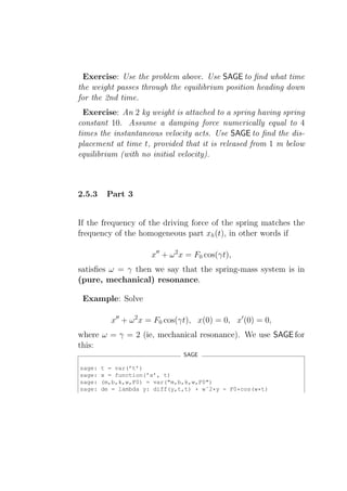
This is displayed below:

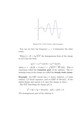
100. Figure 2.11: A forced undamped spring, with resonance.
Example: Solve
x′′ + ω 2 x = F0 cos(γt), x(0) = 0, x′ (0) = 0,
where ω = 2 and γ = 3 (ie, mechanical resonance). We use
SAGE for this:
SAGE
sage: t = var(’t’)
sage: x = function(’x’, t)
sage: (m,b,k,w,g,F0) = var("m,b,k,w,g,F0")
sage: de = lambda y: diff(y,t,t) + wˆ2*y - F0*cos(g*t)
sage: m = 1; b = 0; k = 4; F0 = 1; w = 2; g = 3
sage: desolve_laplace(de(x(t)),["t","x"],[0,0,0])
’cos(2*t)/5-cos(3*t)/5’
sage: soln = lambda t : cos(2*t)/5-cos(3*t)/5
sage: P = plot(soln(t),0,10)
sage: show(P)
This is displayed below:

101. Figure 2.12: A forced undamped spring, no resonance.
2.6 Applications to simple LRC circuits
An LRC circuit is a closed loop containing an inductor of L hen-
ries, a resistor of R ohms, a capacitor of C farads, and an EMF
(electro-motive force), or battery, of E(t) volts, all connected in
series.
They arise in several engineering applications. For example,
AM/FM radios with analog tuners typically use an LRC circuit
to tune a radio frequency. Most commonly a variable capaci-
tor is attached to the tuning knob, which allows you to change
the value of C in the circuit and tune to stations on different
frequencies [R-cir].
We use the following “dictionary” to translate between the
diagram and the DEs.

102. EE object term in DE units symbol
(the voltage drop)
charge q = i(t) dt coulombs
′
current i=q amps
emf e = e(t) volts V
resistor Rq ′ = Ri ohms Ω
capacitor C −1 q farads
′′ ′
inductor Lq = Li henries
Kirchoff ’s First Law: The algebraic sum of the currents trav-
elling into any node is zero.
Kirchoff ’s Second Law: The algebraic sum of the voltage drops
around any closed loop is zero.
Generally, the charge at time t on the capacitor, q(t), satisfies
the DE
1
Lq ′′ + Rq ′ + q = E(t). (2.7)
C
Example 1: Consider the simple LC circuit given by the fol-
lowing diagram.
Figure 2.13: A simple LC circuit.

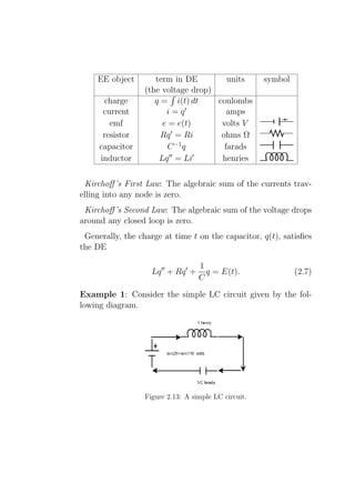
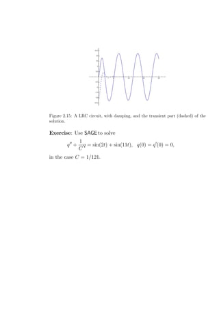
103. According to Kirchoff’s 2nd Law and the above “dictionary”,
this circuit corresponds to the DE
1
q ′′ +
q = sin(2t) + sin(11t).
C
The homogeneous part of the solution is
√ √
qh (t) = c1 cos(t/ C) + c1 sin(t/ C).
If C = 1/4 and C = 1/121 then
1 1
qp (t) = sin(2t) + −1 sin(11t).
C −1 − 4 C − 121
When C = 1/4 and the initial charge and current are both
zero, the solution is
1 161 1
q(t) = − sin(11t) + sin(2t) − t cos(2t).
117 936 4
SAGE
sage: t = var("t")
sage: q = function("q",t)
sage: L,R,C = var("L,R,C")
sage: E = lambda t:sin(2*t)+sin(11*t)
sage: de = lambda y: L*diff(y,t,t) + R*diff(y,t) + (1/C)*y-E(t)
sage: L,R,C=1,0,1/4
sage: de(q(t))
diff(q(t), t, 2) - sin(11*t) - sin(2*t) + 4*q(t)
sage: desolve_laplace(de(q(t)),["t","q"],[0,0,0])
’-sin(11*t)/117+161*sin(2*t)/936-t*cos(2*t)/4’
sage: soln = lambda t: -sin(11*t)/117+161*sin(2*t)/936-t*cos(2*t)/4
sage: P = plot(soln,0,10)
sage: show(P)
This is displayed below:

104. Figure 2.14: A LC circuit, with resonance.
You can see how the frequency ω = 2 dominates the other
terms.
When 0 < R < 2 L/C the homogeneous form of the charge
in (2.7) has the form
qh (t) = c1 eαt cos(βt) + c2 eαt sin(βt),
where α = −R/2L < 0 and β = 4L/C − R2 /(2L). This is
sometimes called the transient part of the solution. The re-
maining terms in the charge are called the steady state terms.
Example: An LRC circuit has a 1 henry inductor, a 2 ohm
resistor, 1/5 farad capacitor, and an EMF of 50 cos(t). If the
initial charge and current is 0, since the charge at time t.
The IVP describing the charge q(t) is
q ′′ + 2q ′ + 5q = 50 cos(t), q(0) = q ′ (0) = 0.
The homogeneous part of the solution is

105. qh (t) = c1 e−t cos(2t) + c2 e−t sin(2t).
The general form of the particular solution using the method of
undetermined coefficients is
qp (t) = A1 cos(t) + A2 sin(t).
Solving for A1 and A2 gives
15 −t
qp (t) = −10e−t cos(2t) − e sin(2t).
2
SAGE
sage: t = var("t")
sage: q = function("q",t)
sage: L,R,C = var("L,R,C")
sage: E = lambda t: 50*cos(t)
sage: de = lambda y: L*diff(y,t,t) + R*diff(y,t) + (1/C)*y-E(t)
sage: L,R,C = 1,2,1/5
sage: de(q(t))
diff(q(t), t, 2) + 2*diff(q(t), t, 1) + 5*q(t) - 50*cos(t)
sage: desolve_laplace(de(q(t)),["t","q"],[0,0,0])
’%eˆ-t*(-15*sin(2*t)/2-10*cos(2*t))+5*sin(t)+10*cos(t)’
sage: soln = lambda t:
eˆ(-t)*(-15*sin(2*t)/2-10*cos(2*t))+5*sin(t)+10*cos(t)
sage: P = plot(soln,0,10)
sage: show(P)
sage: P = plot(soln,0,20)
sage: show(P)
sage: soln_ss = lambda t: 5*sin(t)+10*cos(t)
sage: P_ss = plot(soln_ss,0,10)
sage: soln_tr = lambda t: eˆ(-t)*(-15*sin(2*t)/2-10*cos(2*t))
sage: P_tr = plot(soln_tr,0,10,linestyle="--")
sage: show(P+P_tr)
This plot (the solution superimposed with the transient part of
the solution) is displayed below:

106. Figure 2.15: A LRC circuit, with damping, and the transient part (dashed) of the
solution.
Exercise: Use SAGE to solve
1
q ′′ + q = sin(2t) + sin(11t), q(0) = q ′ (0) = 0,
C
in the case C = 1/121.

107. 2.7 The power series method
2.7.1 Part 1
In this part, we recall some basic facts about power series and
Taylor series. We will turn to solving DEs in part II.
Roughly speaking, power series are simply infinite degree poly-
nomials
∞
2
f (x) = a0 + a1 x + a2 x + ... = ak xk , (2.8)
k=0
for some real or complex numbers a0 , a1 , ... The number ak is
called the coefficient of xk , for k = 0, 1, .... Let us ignore for
the moment the precise meaning of this infinite sum (How do
you associate a value to an infinite sum? Does the sum converge
for some values of x? If so, for which values? ...) We will return
to that later.
First, some motivation. Why study these? This type of func-
tion is convenient for several reasons
• it is easy to differentiate (term-by-term):
∞ ∞
′ 2 k−1
f (x) = a1 +2a2 x+3a3 x +... = kak x = (k+1)ak+1 xk ,
k=0 k=0
• it is easy to integrate (term-by-term):
∞ ∞
1 1 1 1
f (x) dx = a0 x+ a1 x2 + a2 x3 +... = ak xk+1 = ak+1 xk ,
2 3 k+1 k
k=0 k=1

108. • if (as is often the case) the ak ’s tend to zero very quickly,
then the sum of the first few terms of the series are often a
good numerical approximation for the function itself,
• power series enable one to reduce the solution of certain dif-
ferential equations down to (often the much easier problem
of) solving certain recurrance relations.
• Power series expansions arise naturally in Taylor’s Theorem
of the Mean: If f (x) is n + 1 times continuously differen-
tiable in (a, x) then there exists a point ξ ∈ (a, x) such
that
′ (x − a)2 ′′
f (x) = f (a) + (x − a)f (a) + f (a) + · · ·
2!
(x − a)n (n) (x − a)n+1 (n+1)
+ f (a) + f (ξ). (2.9)
n! (n + 1)!
The sum
′ (x − a)2 ′′ (x − a)n (n)
Tn (x) = f (a)+(x−a)f (a)+ f (a)+· · ·+ f (a),
2! n!
is called the n-th degree Taylor polynomial of f cen-
tered at a. For the case n = 0, the formula is
f (x) = f (a) + (x − a)f ′ (ξ),
which is just a rearrangement of the terms in the theorem
of the mean,
f (x) − f (a)
f ′ (ξ) = .
x−a

109. Some examples:
• Geometric series:
1
= 1 + x + x2 + x3 + x4 + · · ·
1−x
∞
= xn (2.10)
n=0
To see this, assume |x| < 1 and let n → ∞ in the polyno-
mial identity
2 n−11 − xn+1
1 + x + x + ··· + x = .
1−x
For x ≥ 1, the series does not converge.
• The exponential function:
x2 x3 x4
ex = 1 + x + + + + ···
2 6 24
x2 x3 x4
=1+x+ + + + ···
2! 3! 4!
∞
xn
= (2.11)
n=0
n!
To see this, take f (x) = ex and a = 0 in Taylor’s theorem
d
(2.9), using the fact that dx ex = ex and e0 = 1:
x x2 x3 xn ξ n+1
e =1+x+ + + ··· + + ,
2! 3! n! (n + 1)!

110. for some ξ between 0 and x. Perhaps it is not clear to
everyone that as n becomes larger and larger (x fixed), the
last (“remainder”) term in this sum goes to 0. However,
Stirling’s formula tells us how large the factorial function
grows,
√ n n 1
n! ∼ 2πn (1 + O( )),
e n
so we may indeed take the limit as n → ∞ to get (2.11).
Wikipedia’s entry on “Power series” [P1-ps] has a nice an-
imation showing how more and more terms in the Taylor
polynomials approximate ex better and better.
• The cosine function:
x2 x4 x6
cos x = 1 − + − + ···
2 24 720
x2 x4 x6
=1− + − + ···
2! 4! 6!
∞ 2n
n x
= (−1) (2.12)
n=0
(2n)!
This too follows from Taylor’s theorem (take f (x) = cos x
and a = 0). However, there is another trick: Replace x in
(2.11) by ix and use the fact (“Euler’s formula”) that eix =
cos(x) + i sin(x). Taking real parts gives (2.12). Taking
imaginary parts gives (2.13), below.

111. • The sine function:
x3 x5 x7
sin x = x − + − + ···
6 120 5040
x3 x5 x7
=1− + − + ···
3! 5! 7!
∞ 2n+1
n x
= (−1) (2.13)
n=0
(2n + 1)!
Indeed, you can formally check (using formal term-by-term
differentiation) that
d
− cos(x) = sin(x).
dx
(Alternatively, you can use this fact to deduce (2.13) from
(2.12).)
• The logarithm function:
1 1 1
log(1 − x) = −x − x2 − x3 − x4 + · · ·
2 3 4
∞
1 n
=− x (2.14)
n=0
n
This follows from (2.10) since (using formal term-by-term
integration)
x
1
= − log(1 − x).
0 1−t
SAGE
sage: taylor(sin(x), x, 0, 5)
x - xˆ3/6 + xˆ5/120

112. sage: P1 = plot(sin(x),0,pi)
sage: P2 = plot(x,0,pi,linestyle="--")
sage: P3 = plot(x-xˆ3/6,0,pi,linestyle="-.")
sage: P4 = plot(x-xˆ3/6+xˆ5/120,0,pi,linestyle=":")
sage: T1 = text("x",(3,2.5))
sage: T2 = text("x-xˆ3/3!",(3.5,-1))
sage: T3 = text("x-xˆ3/3!+xˆ5/5!",(3.7,0.8))
sage: T4 = text("sin(x)",(3.4,0.1))
sage: show(P1+P2+P3+P4+T1+T2+T3+T4)
This is displayed below:
Figure 2.16: Taylor polynomial approximations for sin(x).
Exercise: Use SAGE to plot successive Taylor polynomial ap-
proximations for cos(x).
Finally, we turn to the meaning of these sums. How do you
associate a value to an infinite sum? Does the sum converge for
some values of x? If so, for which values? . We will (for the
most part) answer all of these.
First, consider our infinite power series f (x) in (2.8), where the
ak are all given and x is fixed for the momemnt. The partial

113. sums of this series are
f0 (x) = a0 , f1 (x) = a0 + a1 x, f2 (x) = a0 + a1 x + a2 x2 , · · · .
We say that the series in (2.8) converges at x if the limit of
partial sums
lim fn (x)
n→∞
exists. There are several tests for determining whether or not a
series converges. One of the most commonly used tests is the
Root test: Assume
L = lim |ak xk |1/k = |x| lim |ak |1/k
k→∞ k→∞
exists. If L < 1 then the infinite power series f (x) in (2.8)
converges at x. In general, (2.8) converges for all x satisfying
− lim |ak |−1/k < x < lim |ak |−1/k .
k→∞ k→∞
The number limk→∞ |ak |−1/k (if it exists, though it can be ∞) is
called the radius of convergence.
Example: The radius of convergence of ex (and cos(x) and
sin(x)) is ∞. The radius of convergence of 1/(1−x) (and log(1+
x)) is 1.
Example: The radius of convergence of
∞
k7 + k + 1 k
f (x) = x
2k + k 2
k=0
can be determined with the help of SAGE . We want to compute

114. k 7 + k + 1 −1/k
lim | k | .
k→∞ 2 + k2
SAGE
sage: k = var(’k’)
sage: limit(((kˆ7+k+1)/(2ˆk+kˆ2))ˆ(-1/k),k=infinity)
2
In other words, the series converges for all x satisfying −2 <
x < 2.
Exercise: Use SAGE to find the radius of convergence of
∞
k 3 + 1 2k
f (x) = x
3k + 1
k=0
2.7.2 Part 2
In this part, we solve some DEs using power series.
We want to solve a problem of the form
y ′′ (x) + p(x)y ′ (x) + y(x) = f (x), (2.15)
in the case where p(x), q(x) and f (x) have a power series expan-
sion. We will call a power series solution a series expansion
for y(x) where we have produced some algorithm or rule which
enables us to compute as many of its coefficients as we like.

115. Solution strategy: Write y(x) = a0 + a1 x + a2 x2 + ... =
∞ k
k=0 ak x , for some real or complex numbers a0 , a1 , ....
• Plug the power series expansions for y, p, q, and f into the
DE (2.15).
• Comparing coeffiients of like powers of x, derive relations
between the aj ’s.
• Using these recurrance relations [R-ps] and the ICs, solve
for the coefficients of the power series of y(x).
Example: Solve y ′ − y = 5, y(0) = −4, using the power series
method.
This is easy to solve by undetermined coefficients: yh (x) = c1 ex
and yp (x) = A1 . Solving for A1 gives A1 = −5 and then solving
for c1 gives −4 = y(0) = −5 + c1 e0 so c1 = 1 so y = ex − 5.
Solving this using power series, we compute
∞
y ′ (x) = a1 + 2a2 x + 3a3 x2 + ... = k=0 (k + 1)ak+1 xk
−y(x) = −a0 − a1 x − a2 x2 − ... = ∞ −ak xk
k=0
− − −− −− − − − − − − − − − − − − − − − − − − − − − − −−
5 = (−a0 + a1 ) + (−a1 + 2a2 )x + ... = ∞ (−ak + (k + 1)ak+1 )xk
k=0
Comparing coefficients,
• for k = 0: 5 = −a0 + a1 ,
• for k = 1: 0 = −a1 + 2a2 ,
• for general k: 0 = −ak + (k + 1)ak+1 for k > 0.

116. The IC gives us −4 = y(0) = a0 , so
a0 = −4, a1 = 1, a2 = 1/2, a3 = 1/6, · · · , ak = 1/k!.
This implies
y(x) = −4 + x + x/2 + · · · + xk /k! + · · · = −5 + ex ,
which is in agreement from the previous discussion.
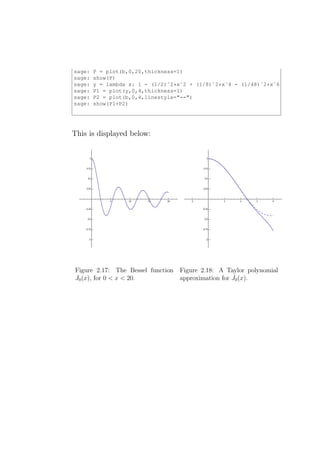
Example: Solve Bessel’s equation [B-ps] of the 0-th order,
x2 y ′′ + xy ′ + x2 y = 0, y(0) = 1, y ′ (0) = 0,
using the power series method.
This DE is so well-known (it has important applications to
physics and engineering) that the series expansion has already
been worked out (most texts on special functions or differential
equations have this but an online reference is [B-ps]). Its Taylor
series expansion around 0 is:
∞
(−1)m x 2m
J0 (x) =
m=0
m!2 2
for all x. We shall see below that y(x) = J0 (x).
Let us try solving this ourselves using the power series method.
We compute
x2 y ′′ (x) = 0 + 0 · x + 2a2 x2 + 6a3 x3 + 12a4 x4 + ... = ∞ (k + 2)(k +
k=0
∞
xy ′ (x) = 2 3
0 + a1 x + 2a2 x + 3a3 x + ... = k=0 kak x k
x2 y(x) = 0 + 0 · x + a0 x2 + a1 x3 + ... = ∞ ak−2 xk
k=2
− − −− −− − − − − − − − − − − − − − − − − − − − − − − −−
0 = 0 + a1 x + (a0 + 4a2 )x2 + ..... = a1 x + ∞ (ak−2 + k 2 ak )xk .
k=2

117. By the ICs, a0 = 1, a1 = 0. Comparing coefficients,
k 2 ak = −ak−2 , k ≥ 2,
which implies
1 1 1 1 1 1
a2 = −( )2 , a3 = 0, a4 = ( · )2 , a5 = 0, a6 = −( · · )2 , · · · .
2 2 4 2 4 6
In general,
1
a2k = (−1)k 2−2k , a2k+1 = 0,
k!2
for k ≥ 1. This is in agreement with the series above for J0 .
Some of this computation can be formally done in SAGE using
power series rings.
SAGE
sage: R6.<a0,a1,a2,a3,a4,a5,a6> = PolynomialRing(QQ,7)
sage: R.<x> = PowerSeriesRing(R6)
sage: y = a0 + a1*x + a2*xˆ2 + a3*xˆ3 + a4*xˆ4 + a5*xˆ5 +
a6*xˆ6 + O(xˆ7)
sage: y1 = y.derivative()
sage: y2 = y1.derivative()
sage: xˆ2*y2 + x*y1 + xˆ2*y
a1*x + (a0 + 4*a2)*xˆ2 + (a1 + 9*a3)*xˆ3 + (a2 + 16*a4)*xˆ4 +
(a3 + 25*a5)*xˆ5 + (a4 + 36*a6)*xˆ6 + O(xˆ7)
This is consistent with our “paper and pencil” computations
above.
SAGE knows quite a few special functions, such as the various
types of Bessel functions.
SAGE
sage: b = lambda x:bessel_J(x,0)

118. sage: P = plot(b,0,20,thickness=1)
sage: show(P)
sage: y = lambda x: 1 - (1/2)ˆ2*xˆ2 + (1/8)ˆ2*xˆ4 - (1/48)ˆ2*xˆ6
sage: P1 = plot(y,0,4,thickness=1)
sage: P2 = plot(b,0,4,linestyle="--")
sage: show(P1+P2)
This is displayed below:
Figure 2.17: The Bessel function Figure 2.18: A Taylor polynomial
J0 (x), for 0 < x < 20. approximation for J0 (x).

119. Exercise: Use SAGE to find the first 5 terms in the power series
solution to y ′′ + y = 0, y(0) = 1, y ′ (0) = 0. Plot this Taylor
polynomial approximation over −π < x < π.

120. 2.8 The Laplace transform method
2.8.1 Part 1
The Laplace transform (LT) of a function f (t), defined for all
real numbers t ≥ 0, is the function F (s), defined by:
∞
F (s) = L [f (t)] = e−st f (t) dt.
0
This is named for Pierre-Simon Laplace, one of the best French
mathematicians in the mid-to-late 18th century [L-lt], [LT-lt].
The LT sends “nice” functions of t (we will be more precise later)
to functions of another variable s. It has the wonderful property
that it transforms constant-coefficient differential equations in t
to algebraic questions in s.
The LT has two very familiar properties: Just as the integral
of a sum is the sum of the integrals, the Laplace transform of a
sum is the sum of Laplace transforms:
L [f (t) + g(t)] = L [f (t)] + L [g(t)]
Just as constant factor can be taken outside of an integral, the
LT of a constant times a function is that constant times the LT
of that function:
L [af (t)] = aL [f (t)]
In other words, the LT is linear.
For which functions f is the LT actually defined on? We want
the indefinite integral to converge, of course. A function f (t) is
of exponential order α if there exist constants t0 and M such

121. that
|f (t)| < M eαt , for all t > t0 .
t
If 0 0 f (t) dt exists and f (t) is of exponential order α then the
Laplace transform L [f ] (s) exists for s > α.
Example 2.8.1. Consider the Laplace transform of f (t) = 1.
The LT integral converges for s > 0.
∞
L [f ] (s) = e−st dt
0
∞
1
= − e−st
s 0
1
=
s
Example 2.8.2. Consider the Laplace transform of f (t) = eat .
The LT integral converges for s > a.
∞
L [f ] (s) = e(a−s)t dt
0
∞
1 (a−s)t
= − e
s−a 0
1
=
s−a
Example 2.8.3. Consider the Laplace transform of the unit step
(Heaviside) function,
0 for t < c
u(t − c) =
1 for t > c,

122. where c > 0.
∞
L[u(t − c)] = e−st H(t − c) dt
0
∞
= e−st dt
c
∞
e−st
=
−s c
e−cs
= for s > 0
s
The inverse Laplace transform in denoted
f (t) = L−1 [F (s)](t),
where F (s) = L [f (t)] (s).
Example 2.8.4. Consider
1, for t < 2,
f (t) =
0, on t ≥ 2.
We show how SAGE can be used to compute the LT of this.
SAGE
sage: t = var(’t’)
sage: s = var(’s’)
sage: f = Piecewise([[(0,2),1],[(2,infinity),0]])
sage: f.laplace(t, s)
1/s - eˆ(-(2*s))/s
sage: f1 = lambda t: 1
sage: f2 = lambda t: 0
sage: f = Piecewise([[(0,2),f1],[(2,10),f2]])
sage: P = f.plot(rgbcolor=(0.7,0.1,0.5),thickness=3)
sage: show(P)

123. According to SAGE , L [f ] (s) = 1/s − e−2s /s. Note the function
f was redefined for plotting purposes only (the fact that it was
redefined over 0 < t < 10 means that SAGE will plot it over that
range.) The plot of this function is displayed below:
Figure 2.19: The piecewise constant function 1 − u(t − 2).
Next, some properties of the LT.
• Differentiate the definition of the LT with respect to s:
∞
′
F (s) = − e−st tf (t) dt.
0
Repeating this:
∞
dn
n
F (s) = (−1)n e−st tn f (t) dt. (2.16)
ds 0
• In the definition of the LT, replace f (t) by it’s derivative
f ′ (t):
∞
′
L [f (t)] (s) = e−st f ′ (t) dt.
0

124. Now integrate by parts (u = e−st , dv = f ′ (t) dt):
∞ ∞
−st ′
e f (t) dt = f (t)e−st |∞ −
0 f (t)·(−s)·e−st dt = −f (0)+sL [f (t)] (
0 0
Therefore, if F (s) is the LT of f (t) then sF (s) − f (0) is the
LT of f ′ (t):
L [f ′ (t)] (s) = sL [f (t)] (s) − f (0). (2.17)
• Replace f by f ′ in (2.17),
L [f ′′ (t)] (s) = sL [f ′ (t)] (s) − f ′ (0), (2.18)
and apply (2.17) again:
L [f ′′ (t)] (s) = s2 L [f (t)] (s) − sf (0) − f ′ (0), (2.19)
• Using (2.17) and (2.19), the LT of any constant coefficient
ODE
ax′′ (t) + bx′ (t) + cx(t) = f (t)
is
a(s2 L [x(t)] (s) − sx(0) − x′ (0)) + b(sL [x(t)] (s) − x(0)) + cL [x(t)] (s) = F (s),
where F (s) = L [f (t)] (s). In particular, the LT of the
solution, X(s) = L [x(t)] (s), satisfies
X(s) = (F (s) + asx(0) + ax′ (0) + bx(0))/(as2 + bs + c).

125. Note that the denominator is the characteristic polynomial
of the DE.
Moral of the story: it is always very easy to compute the LT
of the solution to any constant coefficient non-homogeneous
linear ODE.
Example 2.8.5. We know now how to compute not only the
LT of f (t) = eat (it’s F (s) = (s − a)−1 ) but also the LT of any
function of the form tn eat by differentiating it:
L teat = −F ′ (s) = (s−a)−2 , L t2 eat = F ′′ (s) = 2·(s−a)−3 , L t3 eat = −F ′ (s) =
and in general
L tn eat = −F ′ (s) = n! · (s − a)−n−1 . (2.20)
Example 2.8.6. Let us solve the DE
x′ + x = t100 e−t , x(0) = 0.
using LTs. Note this would be highly impractical to solve using
undetermined coefficients. (You would have 101 undetermined
coefficients to solve for!)
First, we compute the LT of the solution to the DE. The LT of
the LHS: by (2.20),
L [x′ + x] = sX(s) + X(s),
where F (s) = L [f (t)] (s). For the LT of the RHS, let
1
F (s) = L e−t = .
s+1
By (2.16),

126. d100 100 −t d100 1
F (s) = L t e = 100 .
ds100 ds s + 1
1
The first several derivatives of s+1 are as follows:
d 1 1 d2 1 1 d3 1 1
=− , =2 , = −62 ,
ds s + 1 (s + 1)2 ds2 s + 1 (s + 1)3 ds3 s + 1 (s + 1)4
and so on. Therefore, the LT of the RHS is:
d100 1 1
= 100! .
ds100 s + 1 (s + 1)101
Consequently,
1
X(s) = 100! .
(s + 1)102
Using (2.20), we can compute the ILT of this:
1 1 −1 1 1
x(t) = L−1 [X(s)] = L−1 100! = L 101! = t
(s + 1)102 101 (s + 1)102 101
Example 2.8.7. Let us solve the DE
x′′ + 2x′ + 2x = e−2t , x(0) = x′ (0) = 0,
using LTs.
The LT of the LHS: by (2.20) and (2.18),
L [x′′ + 2x′ + 2x] = (s2 + 2s + 2)X(s),
as in the previous example. The LT of the RHS is:
1
L e−2t = .
s+2

127. Solving for the LT of the solution algebraically:
1
X(s) = .
(s + 2)((s + 1)2 + 1)
The inverse LT of this can be obtained from LT tables after
rewriting this using partial fractions:
1 1 1 s 1 1 1 s+1 1 1
X(s) = · − = · − + .
2 s + 2 2 (s + 1)2 + 1 2 s + 2 2 (s + 1)2 + 1 2 (s + 1)2 + 1
The inverse LT is:
1 −2t 1 −t 1
x(t) = L−1 [X(s)] = · e − · e cos(t) + · e−t sin(t).
2 2 2
We show how SAGE can be used to do some of this.
SAGE
sage: t = var(’t’)
sage: s = var(’s’)
sage: f = 1/((s+2)*((s+1)ˆ2+1))
sage: f.partial_fraction()
1/(2*(s + 2)) - s/(2*(sˆ2 + 2*s + 2))
sage: f.inverse_laplace(s,t)
eˆ(-t)*(sin(t)/2 - cos(t)/2) + eˆ(-(2*t))/2
Exercise: Use SAGE to solve the DE
x′′ + 2x′ + 5x = e−t , x(0) = x′ (0) = 0.

128. 2.8.2 Part 2
In this lecture, we shall focus on two other aspects of Laplace
transforms:
• solving differential equations involving unit step (Heavi-
side) functions,
• convolutions and applications.
It follows from the definition of the LT that if
L
f (t) −→ F (s) = L[f (t)](s),
then
L
f (t)u(t − c) −→ e−cs L[f (t + c)](s), (2.21)
and
L
f (t − c)u(t − c) −→ e−cs F (s). (2.22)
These two properties are called translation theorems.
Example 2.8.8. First, consider the Laplace transform of the
piecewise-defined function f (t) = (t − 1)2 u(t − 1). Using (2.22),
this is
1 −s
L[f (t)] = e−s L[t2 ](s) = 2 e .
s3
Second, consider the Laplace transform of the piecewise-constant
function 
0
 for t < 0,
f (t) = −1 for 0 ≤ t ≤ 2,

1 for t > 2.


129. This can be expressed as f (t) = −u(t) + 2u(t − 2), so
L[f (t)] = −L[u(t)] + 2L[u(t − 2)]
1 1
= − + 2 e−2s .
s s
Finally, consider the Laplace transform of f (t) = sin(t)u(t−π).
Using (2.21), this is
1
L[f (t)] = e−πs L[sin(t+π)](s) = e−πs L[− sin(t)](s) = −e−πs .
s2 +1
The plot of this function f (t) = sin(t)u(t − π) is displayed below:
Figure 2.20: The piecewise continuous function u(t − π) sin(t).
We show how SAGE can be used to compute these LTs.
SAGE
sage: t = var(’t’)
sage: s = var(’s’)
sage: assume(s>0)
sage: f = Piecewise([[(0,1),0],[(1,infinity),(t-1)ˆ2]])
sage: f.laplace(t, s)

130. 2*eˆ(-s)/sˆ3
sage: f = Piecewise([[(0,2),-1],[(2,infinity),2]])
sage: f.laplace(t, s)
3*eˆ(-(2*s))/s - 1/s
sage: f = Piecewise([[(0,pi),0],[(pi,infinity),sin(t)]])
sage: f.laplace(t, s)
-eˆ(-(pi*s))/(sˆ2 + 1)
sage: f1 = lambda t: 0
sage: f2 = lambda t: sin(t)
sage: f = Piecewise([[(0,pi),f1],[(pi,10),f2]])
sage: P = f.plot(rgbcolor=(0.7,0.1,0.5),thickness=3)
sage: show(P)
The plot given by these last few commands is displayed above.
Before turning to differential equations, let us introduce con-
volutions.
Let f (t) and g(t) be continuous (for t ≥ 0 - for t < 0, we
assume f (t) = g(t) = 0). The convolution of f (t) and g(t) is
defined by
t t
(f ∗ g) = f (u)g(t − u) du = f (t − u)g(u) du.
0 0
The convolution theorem states
L[f ∗ g(t)](s) = F (s)G(s) = L[f ](s)L[g](s).
The LT of the convolution is the product of the LTs. (Or, equiv-
alently, the inverse LT of the product is the convolution of the
inverse LTs.)
To show this, do a change-of-variables in the following double
integral:

131. ∞ t
L[f ∗ g(t)](s) = e−st f (u)g(t − u) du dt
0 0
∞ ∞
= e−st f (u)g(t − u) dt du
0 u
∞ ∞
−su
= e f (u) e−s(t−u) g(t − u) dt du
0 u
∞ ∞
−su
= e f (u) du e−sv g(v) dv
0 0
= L[f ](s)L[g](s).
1
Example 2.8.9. Consider the inverse Laplace transform of s3 −s2 .
This can be computed using partial fractions and LT tables.
However, it can also be computed using convolutions.
First we factor the denominator, as follows
1 1 1
= 2 .
s3 − s2 s s−1
We know the inverse Laplace transforms of each term:
1 1
L−1
2
= t, L−1 = et
s s−1
We apply the convolution theorem:
t
−1 1 1
L = uet−u du
s2 s − 1 0
t
t t
=e −ue−u 0 −e t
−e−u du
0
t
= −t − 1 + e
Therefore,

132. 1 1
L−1 2s−1
(t) = et − t − 1.
s
Example 2.8.10. Here is a neat application of the convolution
theorem. Consider the convolution
f (t) = 1 ∗ 1 ∗ 1 ∗ 1 ∗ 1.
What is it? First, take the LT. Since the LT of the convolution
is the product of the LTs:
1
L[1 ∗ 1 ∗ 1 ∗ 1 ∗ 1](s) = (1/s)5 = = F (s).
s5
4!
We know from LT tables that L−1 s5 (t) = t4 , so
1 −1 4! 1
f (t) = L−1 [F (s)] (t) = L (t) = t4 .
4! s5 4!
Now let us turn to solving a DE of the form
ay ′′ + by ′ + cy = f (t), y(0) = y0 , y ′ (0) = y1 . (2.23)
First, take LTs of both sides:
as2 Y (s) − asy0 − ay1 + bsY (s) − by0 + cY (s) = F (s),
so
1 asy0 + ay1 + by0
Y (s) = F (s) + . (2.24)
as2 + bs + c as2 + bs + c
1
The function as2 +bs+c is sometimes called the transfer function
(this is an engineering term) and it’s inverse LT,

133. 1
w(t) = L−1 (t),
as2 + bs + c
the weight function for the DE.
Lemma 2.8.1. If a = 0 then w(t) = 0.
(The only proof I have of this is a case-by-case proof using LT
tables. Case 1 is when the roots of as2 + bs + c = 0 are real and
distinct, case 2 is when the roots are real and repeated, and case
3 is when the roots are complex. In each case, w(0) = 0. The
verification of this is left to the reader, if he or she is interested.)
By the above lemma and the first derivative theorem,
s
w′ (t) = L−1 (t).
as2 + bs + c
Using this and the convolution theorem, the inverse LT of
(2.24) is
y(t) = (w ∗ f )(t) + ay0 · w′ (t) + (ay1 + by0 ) · w(t). (2.25)
This proves the following fact.
Theorem 2.8.1. The unique solution to the DE (2.23) is (2.25).
Example 2.8.11. Consider the DE y ′′ +y = 1, y(0) = y ′ (0) = 1.
The weight function is the inverse Laplace transform of s21 ,
+1
so w(t) = sin(t). By (2.25),
t
y(t) = 1 ∗ sin(t) = sin(u) du = − cos(u)|t = 1 − cos(t).
0
0
(Yes, it is just that easy!)

134. If the “impulse” f (t) is piecewise-defined, sometimes the con-
volution term in the formula (2.25) is awkward to compute.
Example 2.8.12. Consider the DE y ′′ − y ′ = u(t − 1), y(0) =
y ′ (0) = 0.
Taking Laplace transforms gives s2 Y (s) − sY (s) = 1 e−s , so
s
1
Y (s) =
3 − s2
e−s .
s
We know from a previous example that
1
L−1 3 − s2
(t) = et − t − 1,
s
so by the translation theorem (2.22), we have
1
y(t) = L−1 3 − s2
e−s (t) = (et−1 −(t−1)−1)·u(t−1) = (et−1 −t)·u(t−1).
s
At this stage, SAGE lacks the functionality to solve this DE.
Exercise: (a) Use SAGE to take the LT of u(t − π/4) cos(t).
(b) Use SAGE to compute the convolution sin(t) ∗ cos(t).

135. Chapter 3
Systems of first order
differential equations
127

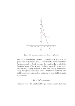
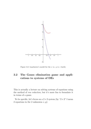
136. 3.1 An introduction to systems of DEs: Lanch-
ester’s equations
The goal of military analysis is a means of reliably predicting
the outcome of military encounters, given some basic informa-
tion about the forces’ status. The case of two combatants in an
“aimed fire” battle was solved during World War I by Frederick
William Lanchester, a British engineer in the Royal Air Force,
who discovered a way to model battle-field casualties using sys-
tems of differential equations. He assumed that if two armies
fight, with x(t) troops on one side and y(t) on the other, the
rate at which soldiers in one army are put out of action is pro-
portional to the troop strength of their enemy. This give rise to
the system of differential equations
x′ (t) = −Ay(t), x(0) = x0 ,
y ′ (t) = −Bx(t), y(0) = y0 ,
where A > 0 and B > 0 are constants (called their fighting effec-
tiveness coefficients) and x0 and y0 are the intial troop strengths.
For some historical examples of actual battles modeled using
Lanchester’s equations, please see references in the paper by
McKay [M-intro].
We show here how to solve these using Laplace transforms.
Example: A battle is modeled by
x′ = −4y, x(0) = 150,
y ′ = −x, y(0) = 90.
(a) Write the solutions in parameteric form. (b) Who wins?
When? State the losses for each side.

137. soln: Take Laplace transforms of both sides:
sL [x (t)] (s) − x (0) = −4 L [y (t)] (s),
sL [x (t)] (s) − x (0) = −4 L [y (t)] (s).
Solving these equations gives
sx (0) − 4 y (0) 150 s − 360
L [x (t)] (s) = = ,
s2 − 4 s2 − 4
−sy (0) + x (0) −90 s + 150
L [y (t)] (s) = − =− .
s2 − 4 s2 − 4
Laplace transform Tables give
x(t) = −15 e2 t + 165 e−2 t
y(t) = 90 cosh (2 t) − 75 sinh (2 t)
Their graph looks like
The “y-army” wins. Solving for x(t) = 0 gives twin = log(11)/4 =
.5994738182..., so the number of survivors is y(twin ) = 49.7493718,
so 49 survive.
Lanchester’s square law: Suppose that if you are more inter-
ested in y as a function of x, instead of x and y as functions of
t. One can use the chain rule form calculus to derive from the
system x′ (t) = −Ay(t), y ′ (t) = −Bx(t) the single equation
dy Bx
= .
dx Ay
This differential equation can be solved by the method of sepa-
ration of variables: Aydy = Bxdx, so
Ay 2 = Bx2 + C,

138. Figure 3.1: Lanchester’s model for the x vs. y battle.
where C is an unknown constant. (To solve for C you must be
given some initial conditions.) The quantity Bx2 is called the
fighting strength of the X-men and the quantity Ay 2 is called the
fighting strength of the Y -men (“fighting strength” is not to be
confused with “troop strength”). This relationship between the
troop strengths is sometimes called Lanchester’s square law
and is sometimes expressed as saying the relative fight strength
is a constant:
Ay 2 − Bx2 = constant.
Suppose your total number of troops is some number T , where

139. x(0) are initially placed in a fighting capacity and T − x(0) are
in a support role. If your tropps outnumber the enemy then you
want to choose the number of support units to be the smallest
number such that the fighting effectiveness is not decreasing
(therefore is roughly constant). The remainer should be engaged
with the enemy in battle [M-intro].
A battle between three forces gives rise to the differential equa-
tions
 ′
 x (t) = −A1 y(t) − A2 z(t), x(0) = x0 ,
y ′ (t) = −B1 x(t) − B2 z(t), y(0) = y0 ,
 ′
z (t) = −C1 x(t) − C2 y(t), z(0) = z0 ,
where Ai > 0, Bi > 0, and Ci > 0 are constants and x0 , y0 and
z0 are the intial troop strengths.
Example: Consider the battle modeled by
 ′
 x (t) = −y(t) − z(t), x(0) = 100,
′
y (t) = −2x(t) − 3z(t), y(0) = 100,
 ′
z (t) = −2x(t) − 3y(t), z(0) = 100.
The Y-men and Z-men are better fighters than the X-men, in the
sense that the coefficient of z in 2nd DE (describing their battle
with y) is higher than that coefficient of x, and the coefficient of
y in 3rd DE is also higher than that coefficient of x. However,
as we will see, the worst fighter wins!
Taking Laplace transforms, we obtain the system

 sX(s) + Y (s) + Z(s) = 100
2X(s) + sY (s) + 3Z(s) = 100,
2X(s) + 3Y (s) + sZ(s) = 100,


140. which we solve by row reduction using the augmented matrix
 
s 1 1 100
2 s 3 100 
2 3 s 100
This has row-reduced echelon form
1 0 0 100s+100
 
s2 +3s−4
 0 1 0 100s−200 
s2 +3s−4
100s−200
0 0 1 s2 +3s−4
This means X(s) = 100s+100 and Y (s) = Z(s) = 100s−200 . Taking
s2 +3s−4 s2 +3s−4
inverse LTs, we get the solution: x(t) = 40e + 60e−4t and y(t) =
t
z(t) = −20et + 120e−4t . In other words, the worst fighter wins!
In fact, the battle is over at t = log(6)/5 = 0.35... and at this
time, x(t) = 71.54.... Therefore, the worst fighters, the X-men,
not only won but have lost less than 30% of their men!
Exercise: A battle is modeled by
x′ = −4y, x(0) = 150,
y ′ = −x, y(0) = 40.
(a) Write the solutions in parameteric form. (b) Who wins?
When? State the losses for each side.
Use SAGE to solve this.

141. Figure 3.2: Lanchester’s model for the x vs. y vs z battle.
3.2 The Gauss elimination game and appli-
cations to systems of DEs
This is actually a lecture on solving systems of equations using
the method of row reduction, but it’s more fun to formulate it
in terms of a game.
To be specific, let’s focus on a 2 × 2 system (by “2 × 2” I mean
2 equations in the 2 unknowns x, y):

142. ax + by = r1
(3.1)
cx + dy = r2
Here a, b, c, d, r1 , r2 are given constants. Putting these two equa-
tions down together means to solve them simultaneously, not in-
dividually. In geometric terms, you may think of each equation
above as a line the the plane. To solve them simultaneously,
you are to find the point of intersection (if it exists) of these two
lines. Since a, b, c, d, r1 , r2 have not been specified, it is conceiv-
able that there are
• no solutions (the lines are parallel but distinct),
• infinitely many solutions (the lines are the same),
• exactly one solution (the lines are distinct and not parallel).
“Usually” there is exactly one solution. Of course, you can solve
this by simply manipulating equations since it is such a low-
dimensional system but the object of this lecture is to show you
a method of solution which is “scalable” to “industrial-sized”
problems (say 1000 × 1000 or larger).
Strategy:
Step 1: Write down the augmented matrix of (3.1):
a b r1
A=
c d r2
This is simply a matter of stripping off the unknowns and record-
ing the coefficients in an array. Of course, the system must be
written in “standard form” (all the terms with “x” get aligned
together, ...) to do this correctly.

143. Step 2: Play the Gauss elimination game (described below) to
computing the row reduced echelon form of A, call it B say.
Step 3: Read off the solution from the right-most column of B.
The Gauss Elimination Game
Legal moves: These actually apply to any m × n matrix A with
m < n.
1. Ri ↔ Rj : You can swap row i with row j.
2. cRi → Ri (c = 0): You can replace row i with row i mul-
tiplied by any non-zero constant c. (Don’t confuse this c
with the c in (3.1)).
3. cRi + Rj → Ri (c = 0): You can replace row i with row i
multiplied by any non-zero constant c plus row j, j = i.
Note that move 1 simply corresponds to reordering the system
of equations (3.1)). Likewise, move 2 simply corresponds to
scaling equation i in (3.1)). In general, these “legal moves”
correspond to algebraic operations you would perform on (3.1))
to solve it. However, there are fewer symbols to push around
when the augmented matrix is used.
Goal: You win the game when you can achieve the following
situation. Your goal is to find a sequence of legal moves leading
to a matrix B satisfying the following criteria:
1. all rows of B have leaading non-zero term equal to 1 (the
position where this leading term in B occurs is called a
pivot position),
2. B contains as many 0’s as possible
3. all entries above and below a pivot position must be 0,

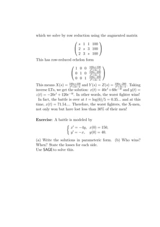
144. 4. the pivot position of the ith row is to the left and above
the pivot position of the (i + 1)st row (therefore, all entries
below the diagonal of B are 0).
This matrix B is unique (this is a theorem which you can find
in any text on elementary matrix theory or linear algebra1 ) and
is called the row reduced echelon form of A, sometimes written
rref (A).
Two comments: (1) If you are your friend both start out play-
ing this game, it is likely your choice of legal moves will differ.
That is to be expected. However, you must get the same result
in the end. (2) Often if someone is to get “stuck” it is becuase
they forget that one of the goals is to “kill as many terms as
possible (i.e., you need B to have as many 0’s as possible). If
you forget this you might create non-zero terms in the matrix
while killing others. You should try to think of each move as
being made in order to to kill a term. The exception is at the
very end where you can’t kill any more terms but you want to
do row swaps to put it in diagonal form.
Now it’s time for an example.
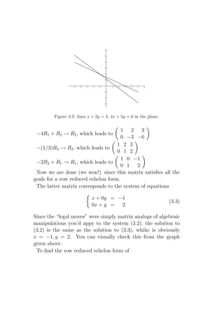
Example: Solve
x + 2y = 3
(3.2)
4x + 5y = 6
The augmented matrix is
1 2 3
A=
4 5 6
One sequence of legal moves is the following:
1
For example, [B-rref] or [H-rref].

145. Figure 3.3: lines x + 2y = 3, 4x + 5y = 6 in the plane.
1 2 3
−4R1 + R2 → R2 , which leads to
0 −3 −6
1 2 3
−(1/3)R2 → R2 , which leads to
0 1 2
1 0 −1
−2R2 + R1 → R1 , which leads to
0 1 2
Now we are done (we won!) since this matrix satisfies all the
goals for a eow reduced echelon form.
The latter matrix corresponds to the system of equations
x + 0y = −1
(3.3)
0x + y = 2
Since the “legal moves” were simply matrix analogs of algebraic
manipulations you’d appy to the system (3.2), the solution to
(3.2) is the same as the solution to (3.3), whihc is obviously
x = −1, y = 2. You can visually check this from the graph
given above.
To find the row reduced echelon form of

146. 1 2 3
4 5 6
using SAGE , just type the following:
SAGE
sage: MS = MatrixSpace(QQ,2,3)
sage: A = MS([[1,2,3],[4,5,6]])
sage: A
[1 2 3]
[4 5 6]
sage: A.echelon_form()
[ 1 0 -1]
[ 0 1 2]
Solving systems using inverses
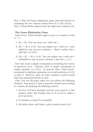
There is another method of solving “square” systems of linear
equations which we discuss next.
One can rewrite the system (3.1) as a single matrix equation
a b x r1
= ,
c d y r2
or more compactly as
AX = r, (3.4)
x r1
where X = and r = . How do you solve (3.4)?
y r2
The obvious this to do (“divide by A”) is the right idea:
x
= X = A−1 r.
y

147. Here A−1 is a matrix with the property that A−1 A = I, the
identity matrix (which satisfies I X = X).
If A−1 exists (and it usually does), how do we compute it?
There are a few ways. One, if using a formula. In the 2 × 2 case,
the inverse is given by
−1
a b 1 d −b
= .
c d ad − bc −c a
There is a similar formula for larger sized matrices but it is so
unwieldy that is is usually not used to compute the inverse. In
the 2 × 2 case, it is easy to use and we see for example,
−1
1 2 1 5 −2 −5/3 2/3
= = .
4 5 −3 −4 1 4/3 −1/3
To find the inverse of
1 2
4 5
using SAGE , just type the following:
SAGE
sage: MS = MatrixSpace(QQ,2,2)
sage: A = MS([[1,2],[4,5]])
sage: A
[1 2]
[4 5]
sage: Aˆ(-1)
[-5/3 2/3]
[ 4/3 -1/3]
A better way to compute A−1 is the following. Compute the
row reduced echelon form of the matrix (A, I), where I is the

148. identity matrix of the same size as A. This new matrix will
be (if the inverse exists) (I, A−1 ). You can read off the inverse
matrix from this.
Here is an example.
Example Solve
x + 2y = 3
4x + 5y = 6
using matrix inverses.
This is
1 2 x 3
= ,
4 5 y 6
so
−1
x 1 2 3
= .
y 4 5 6
To compute the inverse matrix, apply the Gauss elimination
game to
1 2 1 0
4 5 0 1
Using the same sequence of legal moves as in the previous ex-
ample, we get
1 2 1 0
−4R1 + R2 → R2 , which leads to
0 −3 −4 1
1 2 1 0
−(1/3)R2 → R2 , which leads to
0 1 4/3 −1/3
1 0 −5/3 2/3
−2R2 + R1 → R1 , which leads to .
0 1 4/3 −1/3
Therefore the inverse is

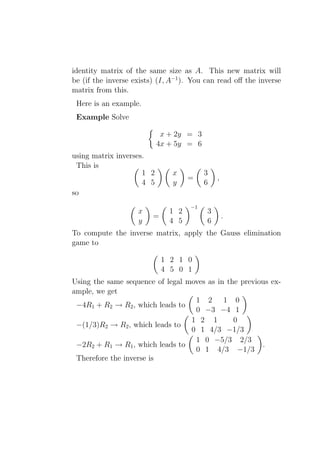
149. −5/3 2/3
A−1 = .
4/3 −1/3
Now, to solve the system, compute
−1
x 1 2 3 −5/3 2/3 3 −1
= = = .
y 4 5 6 4/3 −1/3 6 2
To make SAGE do the above computation, just type the follow-
ing:
SAGE
sage: MS = MatrixSpace(QQ,2,2)
sage: A = MS([[1,2],[4,5]])
sage: V = VectorSpace(QQ,2)
sage: v = V([3,6])
sage: Aˆ(-1)*v
(-1, 2)
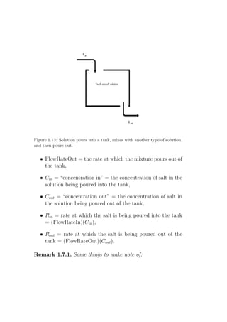
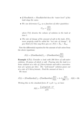
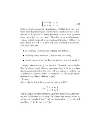
Application: Solving systems of DEs
Suppose we have a system of DEs in “standard form”
x′ = ax + by + f (t), x(0) = x0 ,
(3.5)
y ′ = cx + dy + g(t), y(0) = y0 ,
where a, b, c, d, x0 , y0 are given constants and f (t), g(t) are given
“nice” functions. (Here “nice” will be left vague but basically
we don’t want these functions to annoy us with any bad be-
haviour while trying to solve the DEs by the method of Laplace
transforms.)
One way to solve this system if to take Laplace transforms of
both sides. If we let

150. X(s) = L[x(t)](s), Y (s) = L[y(t)](s), F (s) = L[f (t)](s), G(s) = L[g(t)](s),
then (3.5) becomes
sX(s) − x0 = aX(s) + bY (s) + F (s),
(3.6)
sY (s) − y0 = cX(s) + dY (s) + G(s).
This is now a 2 × 2 system of linear equations in the unknowns
X(s), Y (s) with augmented matrix
s − a −b F (s) + x0
A= .
−c s − d G(s) + y0
Example: Solve
x′ = −y + 1, x(0) = 0,
y ′ = −x + t, y(0) = 0,
The augmented matrix is
s 1 1/s
A= .
1 s 1/s2
The row reduced echelon form of this is
1 0 1/s2
.
0 1 0
Therefore, X(s) = 1/s2 and Y (s) = 0. Taking inverse Laplace
transforms, we see that the solution to the system is x(t) = t
and y(t) = 0. It is easy to check that this is indeed the solution.
To make SAGE compute the row reduced echelon form, just
type the following:

151. SAGE
sage: R = PolynomialRing(QQ,"s")
sage: F = FractionField(R)
sage: s = F.gen()
sage: MS = MatrixSpace(F,2,3)
sage: A = MS([[s,1,1/s],[1,s,1/sˆ2]])
sage: A.echelon_form()
[ 1 0 1/sˆ2]
[ 0 1 0]
To make SAGE compute the Laplace transform, just type the
following:
SAGE
sage: maxima("laplace(1,t,s)")
1/s
sage: maxima("laplace(t,t,s)")
1/sˆ2
To make SAGE compute the inverse Laplace transform, just
type the following:
SAGE
sage: maxima("ilt(1/sˆ2,s,t)")
t
sage: maxima("ilt(1/(sˆ2+1),s,t)")
sin(t)
Example: Solve
x′ = −4y, x(0) = 400,
y ′ = −x, y(0) = 100,

152. This models a battle between “x-men” and “y-men”, where the
“x-men” die off at a higher rate than the “y-men” (but there
are more of them to begin with too).
The augmented matrix is
s 4 400
A= .
1 s 100
The row reduced echelon form of this is
400(s−1)
1 0 s2 −4
100(s−4) .
0 1 s2 −4
Therefore,
s 2 s 2
X(s) = 400 − 200 2 , Y (s) = 100 2 − 200 2 .
s2 − 4 s −4 s −4 s −4
Taking inverse Laplace transforms, we see that the solution to
the system is x(t) = 400 cosh(2t) − 200 sinh(2t) and y(t) =
100 cosh(2t) − 200 sinh(2t). The “x-men” win and, in fact,
x(0.275) = 346.4102..., y(0.275) = −0.1201... .
Question: What is x(t)2 − 4y(t)2 ? (Hint: It’s a constant. Can
you explain this?)
To make SAGE plot this just type the following:
SAGE
sage: f = lambda x: 400*cosh(2*x)-200*sinh(2*x)
sage: g = lambda x: 100*cosh(2*x)-200*sinh(2*x)
sage: P = plot(f,0,1)
sage: Q = plot(g,0,1)
sage: show(P+Q)

153. sage: g(0.275)
-0.12017933629675781
sage: f(0.275)
346.41024490088557
Figure 3.4: curves x(t) = 400 cosh(2t) − 200 sinh(2t), y(t) = 100 cosh(2t) −
200 sinh(2t) along the t-axis.
Example: The displacement from equilibrium (respectively)
for coupled springs attached to a wall on the left
coupled springs
|------////---|mass1|----/////----|mass2|

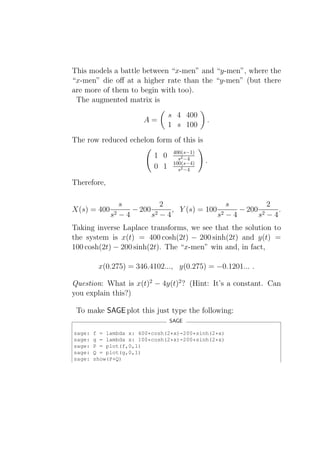
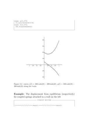
154. spring1 spring2
is modeled by the system of 2nd order ODEs
m1 x′′ + (k1 + k2 )x1 − k2 x2 = 0,
1 m2 x′′ + k2 (x2 − x1 ) = 0,
2
where x1 denotes the displacement from equilibrium of mass
1, denoted m1 , x2 denotes the displacement from equilibrium
of mass 2, denoted m2 , and k1 , k2 are the respective spring
constants [CS-rref].
As another illustration of solving linear systems of equations to
solving systems of linear 1st order DEs, we use SAGE to solve the
above problem with m1 = 2, m2 = 1, k1 = 4, k2 = 2, x1 (0) = 3,
x′1 (0) = 0, x2 (0) = 3, x′2 (0) = 0.
Soln: Take Laplace transforms of the first DE (for simplicity
of notation, let x = x1 , y = x2 ):
SAGE +Maxima
sage: _ = maxima.eval("x2(t) := diff(x(t),t, 2)")
sage: maxima("laplace(2*x2(t)+6*x(t)-2*y(t),t,s)")
2*(-?%at(’diff(x(t),t,1),t=0)+sˆ2*?%laplace(x(t),t,s)-x(0)*s)-2*?%laplace(y(t),t,s)+6*?%laplace(x(t),t,s)
This says −2x′1 (0) + 2s2 ∗ X1 (s) − 2sx1 (0) − 2X2 (s) + 2X1 (s) = 0
(where the Laplace transform of a lower case function is the
upper case function). Take Laplace transforms of the second
DE:
SAGE +Maxima
sage: _ = maxima.eval("y2(t) := diff(y(t),t, 2)")
sage: maxima("laplace(y2(t)+2*y(t)-2*x(t),t,s)")
-?%at(’diff(y(t),t,1),t=0)+sˆ2*?%laplace(y(t),t,s)+2*?%laplace(y(t),t,s)-2*?%laplace(x(t),t,s)-y(0)*s
This says s2 X2 (s) + 2X2 (s) − 2X1 (s) − 3s = 0. Solve these two
equations:

155. SAGE
sage: s,X,Y = var(’s X Y’)
sage: eqns = [(2*sˆ2+6)*X-2*Y == 6*s, -2*X +(sˆ2+2)*Y == 3*s]
sage: solve(eqns, X,Y)
[[X == (3*sˆ3 + 9*s)/(sˆ4 + 5*sˆ2 + 4),
Y == (3*sˆ3 + 15*s)/(sˆ4 + 5*sˆ2 + 4)]]
This says X1 (s) = (3s3 + 9s)/(s4 + 5s2 + 4), X2 (s) = (3s3 +
15s)/(s4 + 5s2 + 4). Take inverse Laplace transforms to get the
answer:
SAGE
sage: s,t = var(’s t’)
sage: inverse_laplace((3*sˆ3 + 9*s)/(sˆ4 + 5*sˆ2 + 4),s,t)
cos(2*t) + 2*cos(t)
sage: inverse_laplace((3*sˆ3 + 15*s)/(sˆ4 + 5*sˆ2 + 4),s,t)
4*cos(t) - cos(2*t)
Therefore, x1 (t) = cos(2t) + 2 cos(t), x2 (t) = 4 cos(t) − cos(2t).
Using SAGE , this can be plotted parametrically using
SAGE
sage: P = parametric_plot([cos(2*t) + 2*cos(t),4*cos(t) - cos(2*t)],0,3)
sage: show(P)
You can also try
SAGE +Maxima
sage.: maxima.plot2d(’cos(2*x) + 2*cos(x)’,’[x,0,1]’,’[plot_format, openmath]’)
for the output of a slightly different looking plotting program.

156. Figure 3.5: curves x(t) = cos(2 ∗ t) + 2 ∗ cos(t), y(t) = 4 ∗ cos(t) − cos(2 ∗ t)
along the t-axis.
Exercise: Solve

 x + 2y + z = 1
−x + 2y − z = 2
y + 2z = 3

using (a) row reduction and SAGE , (b) matrix inverses and
SAGE .

157. 3.3 Eigenvalue method for systems of DEs
Motivation
First, we shall try to motivate the study of eigenvalues and
eigenvectors. This section hopefully will convince you that
• diagonal matrices are wonderful,
• conjugation is very natural,
• if our goal in life is to conjugate a given square matrix ma-
trix into a diagonal one, then eigenvalues and eigenvectors
are also natural.
Diagonal matrices are wonderful: We’ll focus for simplicity on
the 2 × 2 case, but everything applies to the general case.
• Addition is easy:
a1 0 b1 0 a1 + b1 0
+ = .
0 a2 0 b2 0 a2 + b2
• Multiplication is easy:
a1 0 b1 0 a1 · b1 0
· = .
0 a2 0 b2 0 a2 · b2
• Powers are easy:
n
a1 0 an 0
1
= .
0 a2 0 an2

158. • You can even exponentiate them:
a1 0 1 0 a1 0
exp(t ) = +t
0 a2 0 1 0 a2
2 3
1 2 a1 0 1 a1 0
+ 2! t + 3! t3 + ...
0 a2 0 a2
1 0 ta1 0
= +
0 1 0 ta2
1 2 2 1 3 3
ta 0 3! t a1 0
+ 2! 1 1 2 2 + 1 3 3 + ..
0 2! t a2 0 3! t a2
exp(ta1 ) 0
= .
0 exp(ta2 )
So, diagonal matrices are wonderful.
Conjugation is natural. You and your friend are piloting a rocket
in space. You handle the controls, your friend handles the map.
To communicate, you have to “change coordinates”. Your coor-
dinates are those of the rocketship (straight ahead is one direc-
tion, to the right is another). Your friends coordinates are those
of the map (north and east are map directions). Changing co-
ordinates corresponds algebraically to conjugating by a suitable
matrix. Using an example, we’ll see how this arises in a specific
case.
Your basis vectors are
v1 = (1, 0), v2 = (0, 1),
which we call the “v-space coordinates”, and the map’s basis
vectors are

159. w1 = (1, 1), w2 = (1, −1),
which we call the “w-space coordinates”.
Figure 3.6: basis vectors v1 , v2 and w1 , w2 .
For example, the point (7, 3) is, in v-space coordinates of course
(7, 3) but in the w-space coordinates, (5, 2) since 5w1 + 2w2 =
1 1 5
7v1 + 3v2 . Indeed, the matrix A = sends to
1 −1 2
7
.
3

160. Suppose we flip about the 45o line (the “diagonal”) in each
coordinate system. In the v-space:
av1 + bv2 −→ bv1 + av2 ,
a 0 1 a
−→ .
b 1 0 b
0 1
In other words, in v-space, the “flip map” is .
1 0
In the w-space:
wv1 + wv2 −→ aw1 − bw2 ,
a 1 0 a
−→ .
b 0 −1 b
1 0
In other words, in w-space, the “flip map” is .
0 −1
Conjugating by the matrix A converts the “flip map” in w-
space to the the “flip map” in v-space:
1 0 0 1
A· · A−1 = .
0 −1 1 0
Eigenvalues are natural too
Given a matrix A, is there a basis of the underlying space in
which the matrix is diagonal? Given how “wonderful” diagonal
matrices are, it seems clear we should find this basis and these
diagonal entries.
Fact: When the diagonal entries are distinct, the basis elements
are the eigenvectors and the diagonal elements are the eigenval-
ues.

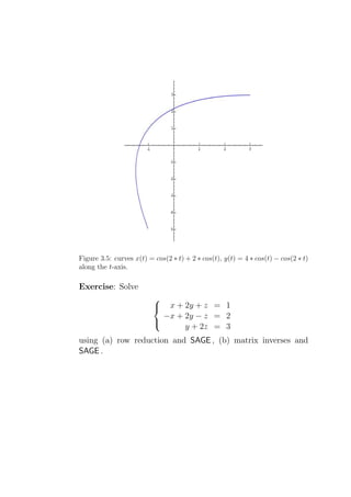
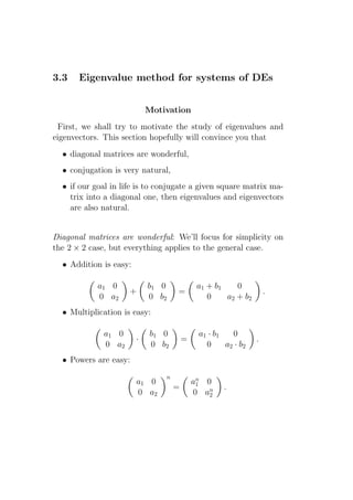
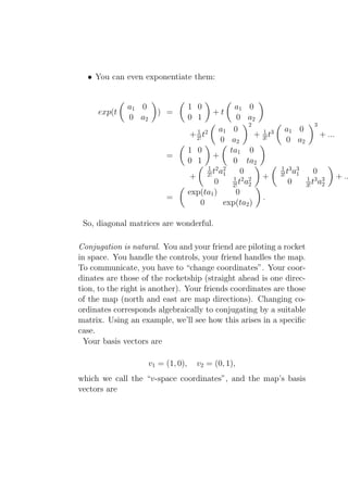
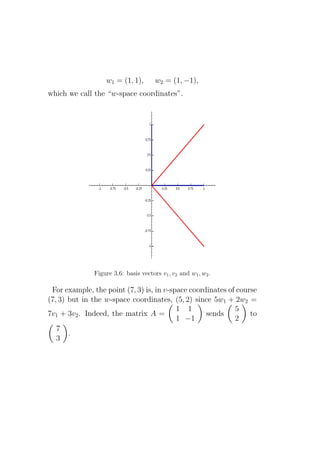
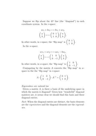
161. Since this section is only intended to be motivation, we shall
not prove this here (see any text on linear algebra, for example
[B-rref] or [H-rref]).
SAGE
sage: MS = MatrixSpace(CC,2,2)
sage: A = MS([[0,1],[1,0]])
sage: A.eigenspaces()
[
(1.00000000000000, [
(1.00000000000000, 1.00000000000000)
]),
(-1.00000000000000, [
(1.00000000000000, -1.00000000000000)
])
]

162. Solution strategy
PROBLEM: Solve
x′ = ax + by, x(0) = x0 ,
y ′ = cx + dy, y(0) = y0 .
soln: Let
a b
A=
c d
In matrix notation, the system of DEs becomes
x0
X ′ = AX, X(0) = ,
y0
x(t)
where X = X(t) = . In a similar manner to how we
y(t)
solved homogeneous constant coefficient 2nd order ODEs ax′′ +
bx′ + cx = 0 by using “Euler’s guess” x = Cert , we try to guess
an exponential: X(t) = ceλt (λ is used instead of r to stick with
notational convention; c in place of C since we need a constant
vector). Plugging this guess into the matrix DE X ′ = AX gives
λceλt = Aceλt , or (cancelling eλt )
Ac = λc.
This means that λ is an eigenvalue of A with eigenvector c.
• Find the eigenvalues. These are the roots of the character-
istic polynomial
a−λ b
p(λ) = det = λ2 − (a + d)λ + (ad − bc).
c d−λ
Call them λ1 , λ2 (in any order you like).

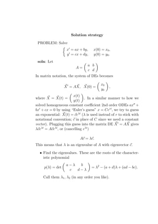
163. You can use the quadratic formula, for example to get them:
a+d (a + d)2 − 4(ad − bc) a+d (a + d)2 − 4(ad − bc)
λ1 = + , λ2 = − .
2 2 2 2
• Find the eigenvectors. If b = 0 then you can use the for-
mulas
b b
v1 = , v2 = .
λ1 − a λ2 − a
In general, you can get them by solving the eigenvector
equation Av = λv.
SAGE
sage: MS = MatrixSpace(CC,2,2)
sage: A = MS([[1,2],[3,4]])
sage: A.eigenspaces()
[
(-0.372281323269014, [
(1.00000000000000, -0.457427107756338)
]),
(5.37228132326901, [
(1.00000000000000, 1.45742710775634)
])
]
• Plug these into the following formulas:
(a) λ1 = λ2 , real:
x(t)
= c1 v1 exp(λ1 t) + c2 v2 exp(λ2 t).
y(t)
(b) λ1 = λ2 = λ, real:
x(t)
= c1 v1 exp(λt) + c2 (v1 t + p) exp(λt),
y(t)

164. where p is any non-zero vector satisfying (A − λI)p =
v1 .
(c) λ1 = α + iβ, complex: write v1 = u1 + iu2 , where u1
and u2 are both real vectors.
x(t)
= c1 [exp(αt) cos(βt)u1 − exp(αt) sin(βt)u2 ]
y(t)
+c2 [− exp(αt) cos(βt)u2 − exp(αt) sin(βt)u1 ].
Examples
Example 3.3.1. Solve
x′ (t)) = x(t)−y(t), y ′ (t) = 4x(t)+y(t), x(0) = −1, y(0) = 1.
Let
1 −1
A=
4 1
and so the characteristc polynomial is
p(x) = det(A − xI) = x2 − 2x + 5.
The eigenvalues are
λ1 = 1 + 2i, λ2 = 1 − 2i,
so α = 1 and β = 2. Eigenvectors v1 , v2 are given by
−1 −1
v1 = , v2 = ,
2i −2i
though we actually only need to know v1 . The real and imaginary
parts of v1 are
−1 0
u1 = , u2 = .
0 2

165. The solution is then
x(t) −c1 exp(t) cos(2t) + c2 exp(t) sin(2t)
=
y(t) −2c1 exp(t) sin(2t) − 2c2 exp(t) cos(2t),
so x(t) = −c1 exp(t) cos(2t)+c2 exp(t) sin(2t) and y(t) = −2c1 exp(t) sin(2t)−
2c2 exp(t) cos(2t).
Since x(0) = −1, we solve to get c1 = 1. Since y(0) = 1,
we get c2 = −1/2. The solution is: x(t) = − exp(t) cos(2t) −
1
2 exp(t) sin(2t) and y(t) = −2 exp(t) sin(2t) + exp(t) cos(2t).
Example 3.3.2. Solve
x′ (t) = −2x(t) + 3y(t), y ′ (t) = −3x(t) + 4y(t).
Let
−2 3
A=
−3 4
and so the characteristc polynomial is
p(x) = det(A − xI) = x2 − 2x + 1.
The eigenvalues are
λ1 = λ2 = 1.
An eigenvector v1 is given by
3
v1 = .
3
Since we can multiply any eigenvector by a non-zero scalar and
get another eigenvector, we shall use instead
1
v1 = .
1

166. r
Let p = be any non-zero vector satisfying (A − λI)p = v1 .
s
This means
−2 − 1 3 r 1
=
−3 4−1 s 1
There are infinitely many possibly solutions but we simply take
r = 0ands = 1/3, so
0
p= .
1/3
The solution is
x(t) 1 1 0
= c1 exp(t) + c2 ( t+ ) exp(t),
y(t) 1 1 1/3
or x(t) = c1 exp(t)+c2 t exp(t) and y(t) = c1 exp(t)+ 1 c2 exp(t)+
3
c2 t exp(t).
Exercises: Use SAGE to find eigenvalues and eigenvectors of
both
1 −1
4 1
and
−2 3
.
−3 4

167. 3.4 Electrical networks using Laplace trans-
forms
Suppose we have an electrical network (i.e., a series of electri-
cal circuits) involving emfs (electromotive forces or batteries),
resistors, capacitors and inductors. We use the following “dic-
tionary” to translate between the diagram and the DEs.
EE object term in DE units symbol
(the voltage drop)
charge q = i(t) dt coulombs
′
current i=q amps
emf e = e(t) volts V
resistor Rq ′ = Ri ohms Ω
capacitor C −1 q farads
inductor Lq ′′ = Li′ henries
Kirchoff ’s First Law: The algebraic sum of the currents trav-
elling into any node is zero.
Kirchoff ’s Second Law: The algebraic sum of the voltage drops
around any closed loop is zero.
Example 1: Consider the simple RC circuit given by the fol-
lowing diagram.
According to Kirchoff’s 2nd Law and the above “dictionary”,
this circuit corresponds to the DE
q ′ + 5q = 2.
The general solution to this is q(t) = 1 + ce−2t , where c is a
constant which depends on the initial charge on the capacitor.

168. Figure 3.7: A simple circuit.
Aside: The convention of assuming that electricity flows from
positive to negative on the terminals of a battery is referred
to as “conventional flow”. The physically-correct but opposite
assumption is referred to as “electron flow”. We shall assume
the “electron flow” convention.
Example 2: Consider the network given by the following di-
agram.
Figure 3.8: A network.
Assume the initial charges are 0.

169. One difference between this circuit and the one above is that
the charges on the three paths between the two nodes (labeled
node 1 and node 2 for convenience) must be labeled. The charge
passing through the 5 ohm resistor we label q1 , the charge on
the capacitor we denote by q2 , and the charge passing through
the 1 ohm resistor we label q3 .
There are three closed loops in the above diagram: the “top
loop”, the “bottom loop”, and the “big loop”. The loops will
be traversed in the “clockwise” direction. Note the “top loop”
looks like the simple circuit given in Example 1 but it cannot
be solved in the same way, since the current passing through
the 5 ohm resistor will affect the charge on the capacitor. This
current is not present in the circuit of Example 1 but it does
occur in the network above.
Kirchoff’s Laws and the above “dictionary” give
 ′
 q3 + 5q2 = 2, q1 (0) = 0,
′
5q1 − 5q2 = 0, q2 (0) = 0,
 ′ ′
5q1 + q3 = 2, q3 (0) = 0.
Notice the minus sign in front of the term associated to the
capacitor (−5q2 ). This is because we are going clockwise, against
the “direction of the current”. Kirchoff’s 1st law says q3 = q1 +q2 .
′ ′ ′
Since q1 (0) = q2 (0) = q3 (0) = 0, this implies q3 = q1 + q2 . After
taking Laplace transforms of the 3 differential equations above,
we get
sQ3 (s) + 5Q2 (s) = 2/s, 5sQ1 (s) − 5Q2 (s) = 0.
Note you don’t need to take th eLT of the 3rd equation since
it is the sum of the first two equations. The LT of the above
q1 + q2 = q3 (Kirchoff’s law) gives Q1 (s) + Q2 (s) − Q3 (s) = 0.

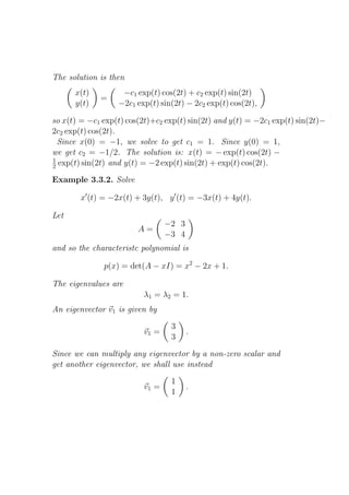
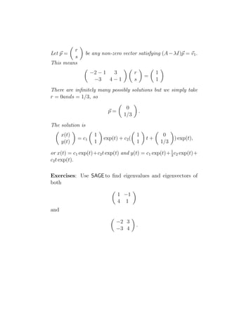
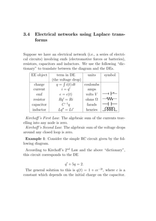
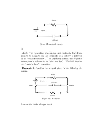
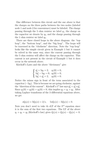
170. We therefore have this matrix equation
    
0 5 s Q1 (s) 2/s
 5s 0 s   Q2 (s)  =  2/s  .
1 1 −1 Q3 (s) 0
The augmented matrix describing this system is
 
0 5 s 2/s
 5s 0 s 2/s 
1 1 −1 0
The row-reduced echelon form is
2/(s3 + 6s2 )
 
1 0 0
0 1 0 2/(s2 + 6s) 
0 0 1 2(s + 1)/(s3 + 6s2 )
Therefore
2 2 2(s + 1)
Q1 (s) = , Q2 (s) = , Q3 (s) = .
s3 + 6s2 s2 + 6s s2 (s + 6)
This implies
q1 (t) = −1/18+e−6t /18+t/3, q2 (t) = 1/3−e−6t /3, q3 (t) = q2 (t)+q1 (t).
This computation can be done in SAGE as well:
SAGE
sage: s = var("s")
sage: MS = MatrixSpace(SymbolicExpressionRing(), 3, 4)
sage: A = MS([[0,5,s,2/s],[5*s,0,s,2/s],[1,1,-1,0]])
sage: B = A.echelon_form(); B

171. [ 1 0 0 2/(5*sˆ2) - (-2/(5*s) - 2/(5*sˆ2))/(5*(-s/5 - 6/5))]
[ 0 1 0 2/(5*s) - (-2/(5*s) - 2/(5*sˆ2))*s/(5*(-s/5 - 6/5)) ]
[ 0 0 1 (-2/(5*s) - 2/(5*sˆ2))/(-s/5 - 6/5) ]
sage: Q1 = B[0,3]
sage: t = var("t")
sage: Q1.inverse_laplace(s,t)
eˆ(-(6*t))/18 + t/3 - 1/18
sage: Q2 = B[1,3]
sage: Q2.inverse_laplace(s,t)
1/3 - eˆ(-(6*t))/3
sage: Q3 = B[2,3]
sage: Q3.inverse_laplace(s,t)
-5*eˆ(-(6*t))/18 + t/3 + 5/18
Example 3: Consider the network given by the following dia-
gram.
Figure 3.9: Another network.
Assume the initial charges are 0.

172. Using Kirchoff’s Laws, you get a system

 i1 − i2 − i3 = 0,
2i1 + i2 + (0.2)i′1 = 6,
(0.1)i′3 − i2 = 0.

Take LTs of these three DEs. You get a 3 × 3 system in the
unknowns I1 (s) = L[i1 (t)](s), I2 (s) = L[i2 (t)](s), and I3 (s) =
L[i3 (t)](s). The augmented matrix of this system is
 
1 −1 −1 0
 2 + s/5 1 0 6/s 
0 −1 s/10 0
(Check this yourself!) The row-reduced echelon form is
 30(s+10)

1 0 0 s(s2 +25s+100)
30
0 1 0 s2 +25s+100 
 
300
0 0 1 s(s2 +25s+100)
Therefore
1 2 3 2 2 1 4
I1 (s) = − − + , I2 (s) = − + , I3 (s) = −
s + 20 s + 5 s s + 20 s + 5 s + 20 s +
This implies
i1 (t) = 3−2e−5t −e−20t , i2 (t) = 2e−5t −2e−20t , i3 (t) = 3−4e−5t +e−20t .
Exercise: Use SAGE to solve for i1 (t), i2 (t), and i3 (t) in the
above problem.

173. Chapter 4
Introduction to partial
differential equations
4.1 Introduction to separation of variables
A partial differential equation (PDE) is an equation satisfied by
an unknown function (called the dependent variable) and its
partial derivatives. The variables you differentiate with respect
to are called the independent variables. If there is only one
independent variable then it is called an ordinary differential
equation.
Examples include
2 2
• the Laplace equation ∂ u + ∂ u = 0, where u is the dependent
∂x2 ∂y 2
variable and x, y are the independent variables,
• the heat equation ut = αuxx ,
• and the wave equation utt = c2 uxx .
All these PDEs are of second order (you have to differentiate
twice to express the equation). Here, we consider a first order
165

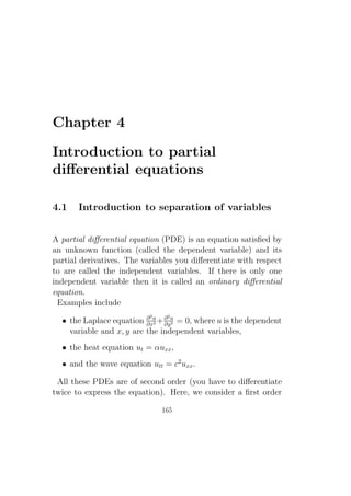
174. PDE which arises in applications and use it to introduce the
method of solution called separation of variables.
The transport or advection equation
Advection is the transport of a some conserved scalar quantity
in a vector field. A good example is the transport of pollutants
or silt in a river (the motion of the water carries these impurities
downstream) or traffic flow.
The advection equation is the PDE governing the motion of
a conserved quantity as it is advected by a given velocity field.
The advection equation expressed mathematically is:
∂u
+ ∇ · (ua) = 0
∂t
where ∇· is the divergence and a is the velocity field of the fluid.
Frequently, it is assumed that ∇ · a = 0 (this is expressed by
saying that the velocity field is solenoidal). In this case, the
above equation reduces to
∂u
+ a · ∇u = 0.
∂t
Assume we have horizontal pipe in which water is flowing at a
constant rate c in the positive x direction. Add some salt to this
water and let u(x, t) denote the concentration (say in lbs/gallon)
at time t. Note that the amount of salt in an interval I of the
pipe is I u(x, t) dx. This concentration satisfies the transport
(or advection) equation:
ut + cux = 0.
(For a derivation of this, see for example Strauss [S-pde], §1.3.)
How do we solve this?

175. Solution 1: D’Alembert noticed that the directional derivative
1 1
of u(x, t) in the direction v = √1+c2 c, 1 is Dv (u) = √1+c2 (cux +
ut ) = 0. Therefore, u(x, t) is constant along the lines in the
direction of v, and so u(x, t) = f (x − ct), for some function f .
We will not use this method of solution in the example below
but it does help visualize the shape of the solution. For instance,
imagine the plot of z = f (x − ct) in (x, t, z) space. The contour
lying above the line x = ct + k (k fixed) is the line of constant
height z = f (k).
Solution 2: The method of separation of variables indicates
that we start by assuming that u(x, t) can be factored:
u(x, t) = X(x)T (t),
for some (unknown) functions X and T . (One can shall work
on removing this assumption later. This assumption “works”
because partial differentiation of functions like x2 t3 is so much
simpler that partial differentiation of “mixed” functions like
sin(x2 + t3 ).) Substituting this into the PDE gives
X(x)T ′ (t) + cX ′ (x)T (t) = 0.
Now separate all the x’s on one side and the t’s on the other
(divide by X(x)T (t)):
T ′ (t) X ′ (x)
= −c .
T (t) X(x)
(This same “trick” works when you apply the separation of vari-
ables method to other linear PDE’s, such as the heat equation
or wave equation, as we will see in later lessons.) It is impossi-
ble for a function of an independent variable x to be identically
equal to a function of an independent variable t unless both are

176. ′
constant. (Indeed, try taking the partial derivative of T (t) with
T
(t)
respect to x. You get 0 since it doesn’t depend on x. Therefore,
′ ′
the partial derivative of −c X (x) is akso 0, so X (x) is a constant!)
X(x) X(x)
′ ′
Therefore, T (t) = −c X (x) = K, for some (unknown) constant
T
(t)
X(x)
K. So, we have two ODEs:
T ′ (t) X ′ (x)
= K, = −K/c.
T (t) X(x)
Therefore, we can converted the PDE into two ODEs. Solving,
we get
T (t) = c1 eKt , X(x) = c2 e−Kx/c ,
K
so, u(x, t) = AeKt−Kx/c = Ae− c (x−ct) , for some constants K
and A (where A is shorthand for c1 c2 ; in terms of D’Alembert’s
K
solution, f (y) = Ae− c (y) ). The “general solution” is a sum of
these (for various A’s and K’s).
This can also be done in SAGE :
SAGE
sage: t = var("t")
sage: T = function("T",t)
sage: K = var("K")
sage: T0 = var("T0")
sage: maxima.de_solve(’diff(T,t) =
K*T’, [’t’,’T’], [0,T0])
T=%eˆ(t*K)*T0
sage: x = var("x")
sage: X = function("X",x)
sage: c = var("c")
sage: X0 = var("X0")
sage: maxima.de_solve(’diff(X,x) =
-cˆ(-1)*K*X’, [’x’,’X’], [0,X0])
X=%eˆ-(x*K/c)*X0
sage: solnX = maxima.de_solve(’diff(X,x) =

177. -cˆ(-1)*K*X’, [’x’,’X’], [0,X0])
sage: solnX.rhs()
%eˆ-(x*K/c)*X0
sage: solnT = maxima.de_solve(’diff(T,t) =
K*T’, [’t’,’T’], [0,T0])
sage: solnT.rhs()
%eˆ(t*K)*T0
sage: solnT.rhs()*solnX.rhs()
%eˆ(t*K-x*K/c)*T0*X0
Example: Assume water is flowing along a horizontal pipe at
3 gal/min in the x direction and that there is an initial con-
centration of salt distributed in the water with concentration of
u(x, 0) = e−x . Using separation of variables, find the concentra-
tion at time t. Plot this for various values of t.
Solution: The method of separation of variables gives the “sep-
arated form” of the solution to the transport PDE as u(x, t) =
AeKt−Kx/c , where c = 3. The initial condition implies
e−x = u(x, 0) = AeK·0−Kx/c = Ae−Kx/3 ,
so A = 1 and K = 3. Therefore, u(x, t) = e3t−x . In other words,
the salt concentration is increasing in time. This makes sense if
you think about it this way: “freeze” the water motion at time
t = 0. There is a lot of salt at the beginning of the pipe and
less and less salt as you move along the pipe. Now go down the
pipe in the x-direction some amount where you can barely tell
there is any salt in the water. Now “unfreeze” the water motion.
Looking along the pipe, you see the concentration is increasing
since the saltier water is now moving toward you.
This is produced using either the Maxima command

178. Figure 4.1: Transport with velocity c = 3.
Maxima
(%i1) plot3d(exp(3*t-x),[x,0,2],[t,0,2],[grid,12,12]);
or the SAGE command
SAGE
sage: maxima.plot3d ("exp(3*t-x)", "[x,0,2]", "[t,0,2]",
"[grid,12,12]", ’[plot_format, openmath]’)
In both cases, wish and tcl/tk must also be installed.
What if the initial concentration was not u(x, 0) = e−x but
instead u(x, 0) = e−x + 3e−5x ? How does the solution to
ut + 3ux = 0, u(x, 0) = e−x + 3e−5x , (4.1)
differ from the method of solution used above? In this case, we
must use the fact that (by superposition) “the general solution”
is of the form

179. u(x, t) = A1 eK1 (t−x/3) + A2 eK2 (t−x/3) + A3 eK3 (t−x/3) + ... , (4.2)
for some constants A1 , K1 , .... To solve this PDE (4.1), we must
answer the following questions: (1) How many terms from (4.2)
are needed? (2) What are the constants A1 , K1 , ...? There are
two terms in u(x, 0), so we can hope that we only need to use
two terms and solve
e−x + 3e−5x = u(x, 0) = A1 eK1 (0−x/3) + A2 eK2 (0−x/3)
for A1 , K1 , A2 , K2 . Indeed, this is possible to solve: A1 = 1,
K1 = 3, A2 = 3, K1 = 15. This gives
u(x, t) = e3(t−x/3) + 3e15(t−x/3) .
Exercise: Using SAGE , solve and plot the solution to the fol-
lowing problem. Assume water is flowing along a horizontal pipe
at 3 gal/min in the x direction and that there is an initial con-
centration of salt distributed in the water with concentration of
u(x, 0) = ex .

180. 4.2 Fourier series, sine series, cosine series
History: Fourier series were discovered by J. Fourier, a French-
man who was a mathematician among other things. In fact,
Fourier was Napolean’s scientific advisor during France’s inva-
sion of Egypt in the late 1800’s. When Napolean returned to
France, he “elected” (i.e., appointed) Fourier to be a Prefect
- basically an important administrative post where he oversaw
some large construction projects, such as highway constructions.
It was during this time when Fourier worked on the theory of
heat on the side. His solution to the heat equation is basically
what undergraduates often learn in a DEs with BVPs class. The
exception being that our understanding of Fourier series now is
much better than what was known in the early 1800’s and some
of these facts, like Dirichlet’s theorem, are covered as well.
Motivation: Fourier series, since series, and cosine series are
all expansions for a function f (x), much in the same way that a
Taylor series a0 + a1 (x − x0 ) + a2 (x − x0 )2 + ... is an expansion.
Both Fourier and Taylor series can be used to approximate f (x).
There are at least three important differences between the two
types of series. (1) For a function to have a Taylor series it
must be differentiable1 , whereas for a Fourier series it does not
even have to be continuous. (2) Another difference is that the
Taylor series is typically not periodic (though it can be in some
cases), whereas a Fourier series is always periodic. (3) Finally,
the Taylor series (when it converges) always converges to the
function f (x), but the Fourier series may not (see Dirichlet’s
1
Remember the formula for the n-th Taylor series coefficient centered at x = x0 -
(n)
an = f n! 0 ) ?
(x

181. theorem below for a more precise description of what happens).
Definitions: Let f (x) be a function defined on an interval of
the real line. We allow f (x) to be discontinuous but the points
in this interval where f (x) is discontinuous must be finite in
number and must be jump discontinuities.
First, we discuss Fourier series. To have a Fourier series you
must be given two things: (1) a “period” P = 2L, (2) a function
f (x) defined on an interval of length 2L, usually we take −L <
x < L (but sometimes 0 < x < 2L is used instead). The Fourier
series of f (x) with period 2L is
∞
a0 nπx nπx
f (x) ∼ + [an cos( ) + bn sin( )],
2 n=1
L L
where an and bn are given by the formulas2 ,
L
1 nπx
an = f (x) cos( ) dx, (4.3)
L −L L
and
1 L nπx
bn = f (x) sin( ) dx. (4.4)
L −L L
Next, we discuss cosine series. To have a cosine series you must
be given two things: (1) a “period” P = 2L, (2) a function f (x)
defined on the interval of length L, 0 < x < L. The cosine
series of f (x) with period 2L is
∞
a0 nπx
f (x) ∼ + an cos( ),
2 n=1
L
where an is given by
2
These formulas were not known to Fourier. To compute the Fourier coefficients an , bn
he used sometimes ingenious round-about methods using large systems of equations.

182. L
2 nπx
an = cos( )f (x) dx.
L 0 L
(This formula is not in your USNA Math Tables.) The cosine
series of f (x) is exactly the same as the Fourier series of the
even extension of f (x), defined by
f (x), 0 < x < L,
feven (x) =
f (−x), −L < x < 0.
Finally, we define sine series. To have a sine series you must
be given two things: (1) a “period” P = 2L, (2) a function f (x)
defined on the interval of length L, 0 < x < L. The sine series
of f (x) with period 2L is
∞
nπx
f (x) ∼ bn sin( ),
n=1
L
where bn is given by
L
2 nπx
bn = sin( )f (x) dx.
L 0 L
The sine series of f (x) is exactly the same as the Fourier series
of the odd extension of f (x), defined by
f (x), 0 < x < L,
fodd (x) =
−f (−x), −L < x < 0.
One last definition: the symbol ∼ is used above instead of =
because of the fact that was pointed out above: the Fourier
series may not converge to f (x). Do you remember right-hand
and left-hand limits from calculus 1? Recall they are denoted
f (x+) = limǫ→0,ǫ>0 f (x + ǫ) and f (x−) = limǫ→0,ǫ>0 f (x − ǫ),

183. resp.. The meaning of ∼ is that the series does necessarily not
converge to the value of f (x) at every point3 . The convergence
proprties are given by the theorem below.
Dirichlet’s theorem4 : Let f (x) be a function as above and
let −L < x < L. The Fourier series of f (x),
∞
a0 nπx nπx
f (x) ∼ + [an cos( ) + bn sin( )],
2 n=1
L L
(where an and bn are as in the formulas (4.3), (4.4)) converges
to
f (x+) + f (x−)
.
2
In other words, the Fourier series of f (x) converges to f (x) only
if f (x) is continuous at x. If f (x) is not continuous at x then
then Fourier series of f (x) converges to the “midpoint of the
jump”.
Examples: (1) If f (x) = 2+x, −2 < x < 2, then the definition
of L implies L = 2. Without even computing the Fourier series,
we can evaluate it using Dirichlet’s theorem.
Question: Using periodicity and Dirichlet’s theorem, find the
value that the Fourier series of f (x) converges to at x = 1, 2, 3.
(Ans: f (x) is continuous at 1, so the FS at x = 1 converges to f (1) = 3 by
Dirichlet’s theorem. f (x) is not defined at 2. It’s FS is periodic with period 4, so at
f (2+)+f (2−) 0+4
x = 2 the FS converges to 2 = 2 = 2. f (x) is not defined at 3. It’s FS
f (−1)+f (−1+) 1+1
is periodic with period 4, so at x = 3 the FS converges to 2 = 2 = 1.)
The formulas (4.3) and (4.4) enable us to compute the Fourier
series coefficients a0 , an and bn . (We skip the details.) These
3
Fourier believed his series converged to the function in the early 1800’s but we now
know this is not always true.
4
Pronounced “Dear-ish-lay”.

184. formulas give that the Fourier series of f (x) is
∞
4 nπ cos (nπ) nπx
f (x) ∼ + −4 sin( ).
2 n=1 n2 π 2 2
The Fourier series approximations to f (x) are
4 πx sin 1 π x
2 sin (π x)
S0 = 2, S1 = 2+ sin( ), S2 = 2+4 −2 , ...
π 2 π π
The graphs of each of these functions get closer and closer to
the graph of f (x) on the interval −2 < x < 2. For instance, the
graph of f (x) and of S8 are given below:
Notice that f (x) is only defined from −2 < x < 2 yet the Fourier
series is not only defined everywhere but is periodic with period
P = 2L = 4. Also, notice that S8 is not a bad approximation to
f (x).
This can also be done in SAGE . First, we define the function.
SAGE
sage: f = lambda x:x+2
sage: f = Piecewise([[(-2,2),f]])
This can be plotted using the command f.plot().show(). Next,
we compute the Fourier series coefficients:
SAGE
sage: f.fourier_series_cosine_coefficient(0,2) # a_0
4
sage: f.fourier_series_cosine_coefficient(1,2) # a_1
0
sage: f.fourier_series_cosine_coefficient(2,2) # a_2
0
sage: f.fourier_series_cosine_coefficient(3,) # a_3

185. 4
3
2
1
–4 –3 –2 –1 0 1 2 3 4
x
Figure 4.2: Graph of f (x) and a Fourier series approximation of f (x).
0
sage: f.fourier_series_sine_coefficient(1,2) # b_1
4/pi
sage: f.fourier_series_sine_coefficient(2,) # b_2
-2/pi
sage: f.fourier_series_sine_coefficient(3,2) # b_3
4/(3*pi)
Finally, the partial Fourier series and it’s plot verses the function
can be computed using the following SAGE commands.
SAGE
sage: f.fourier_series_partial_sum(3,2)
-2*sin(pi*x)/pi + 4*sin(pi*x/2)/pi + 2
sage: P1 = f.plot_fourier_series_partial_sum(15,2,-5,5,linestyle=":")

186. sage: P2 = f.plot(rgbcolor=(1,1/4,1/2))
sage: (P1+P2).show()
The plot (which takes 15 terms of the Fourier series) is given
below.
Figure 4.3: Graph of f (x) = x + 2 and a Fourier series approximation, L = 2.
(2) This time, let’s consider an example of a cosine series. In
this case, we take the piecewise constant function f (x) defined
on 0 < x < 3 by
1, 0 < x < 2,
f (x) =
−1, 2 ≤ x < 3.

187. We see therefore L = 3. The formula above for the cosine series
coefficients gives that
∞
1 sin 2 nπ
3 nπx
f (x) ∼ + 4 cos( ).
3 n=1 nπ 3
The first few partial sums are
√ 1
3 cos 3 π x
S2 = 1/3 + 2 ,
π
√ 1
√
3 cos 3 π x 3 cos 2 π x
3
S3 = 1/3 + 2 − , ...
π π
As before, the more terms in the cosine series we take, the better
the approximation is, for 0 < x < 3. Comparing the picture
below with the picture above, note that even with more terms,
this approximation is not as good as the previous example. The
precise reason for this is rather technical but basically boils down
to the following: roughly speaking, the more differentiable the
function is, the faster the Fourier series converges (and therefore
the better the partial sums of the Fourier series will approximate
f (x)). Also, notice that the cosine series approximation S10 is an
even function but f (x) is not (it’s only defined from 0 < x < 3).
For instance, the graph of f (x) and of S10 are given below:
(3) Finally, let’s consider an example of a sine series. In this
case, we take the piecewise constant function f (x) defined on
0 < x < 3 by the same expression we used in the cosine series
example above.
Question: Using periodicity and Dirichlet’s theorem, find the
value that the sine series of f (x) converges to at x = 1, 2, 3.
(Ans: f (x) is continuous at 1, so the FS at x = 1 converges to f (1) = 1. f (x) is

188. 1
0.5
–6 –4 –2 0 2 4 6
x
–0.5
–1
Figure 4.4: Graph of f (x) and a cosine series approximation of f (x).
f (2+)+f (2−) f (−2+)+f (2−)
not continuous at 2, so at x = 2 the SS converges to 2 = 2 =
−1+1
2 = 0. f (x) is not defined at 3. It’s SS is periodic with period 6, so at x = 3
fodd (3−)+fodd (3+) −1+1
the SS converges to 2 = 2 = 0.)
The formula above for the sine series coefficients give that
∞ 2
cos (nπ) − 2 cos 3 nπ + 1 nπx
f (x) = 2 sin( ).
n=1
nπ 3
The partial sums are
sin (1/3 π x) sin 2 π x
3
S2 = 2 +3 ,
π π
1 2
sin 3 πx sin
sin (π x)
3 πx
S3 = 2 +3 , ... − 4/3
π π π
These partial sums Sn , as n → ∞, converge to their limit about
as fast as those in the previous example. Instead of taking only
10 terms, this time we take 40. Observe from the graph below
that the value of the sine series at x = 2 does seem to be ap-
proaching 0, as Dirichlet’s Theorem predicts. The graph of f (x)
with S40 is

189. 1
0.5
–6 –4 –2 2 4 6
x
–0.5
–1
Figure 4.5: Graph of f (x) and a sine series approximation of f (x).

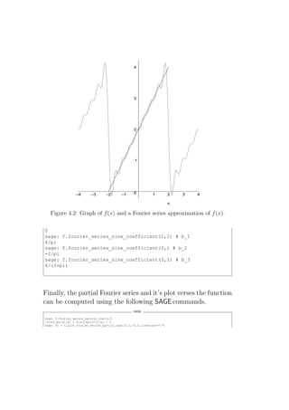
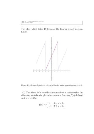
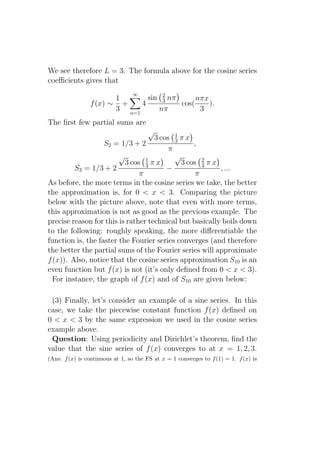
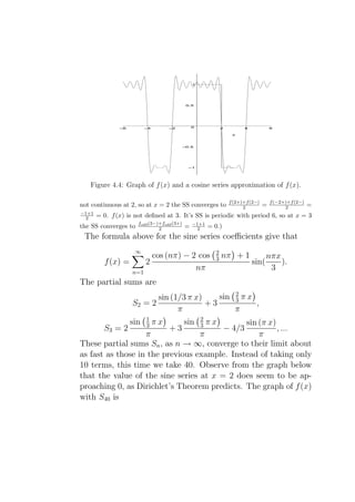
190. Exercise: Let f (x) = x2 , −2 < x < 2 and L = 2. Use SAGE to
compute the first 10 terms of the Fourier series, and plot the
corresponding partial sum. Next plot the partial sum of the
first 50 terms and compare them.
Exercise: What mathematical results do the following SAGE commands
give you? In other words, if you can seen someone typing these
commands into a computer, explain what problem they were
trying to solve.
SAGE
sage: x = var("x")
sage: f0 = lambda x: 0*x
sage: f1 = lambda x: -xˆ0
sage: f2 = lambda x: xˆ0
sage: f = Piecewise([[(-2,0),f1],[(0,3/2),f0],[(3/2,2),f2]])
sage: P1 = f.plot()
sage: a10 = [f.fourier_series_cosine_coefficient(n,2) for n in range(10)]
sage: b10 = [f.fourier_series_sine_coefficient(n,2) for n in range(10)]
sage: fs10 = a10[0]/2 + sum([a10[i]*cos(i*pi*x/2) for i in
range(1,10)]) + sum([b10[i]*sin(i*pi*x/2) for i in range(10)])
sage: P2 = fs10.plot(-4,4,linestyle=":")
sage: (P1+P2).show()
sage:
sage: a50 = [f.fourier_series_cosine_coefficient(n,2) for n in range(50)]
sage: b50 = [f.fourier_series_sine_coefficient(n,2) for n in range(50)]
sage: fs50 = a50[0]/2 + sum([a50[i]*cos(i*pi*x/2) for i in
range(1,50)]) + sum([b50[i]*sin(i*pi*x/2) for i in range(50)])
sage: P3 = fs50.plot(-4,4,linestyle="--")
sage: (P1+P2+P3).show()
sage: a100 = [f.fourier_series_cosine_coefficient(n,2) for n in range(100)]
sage: b100 = [f.fourier_series_sine_coefficient(n,2) for n in range(100)]
sage: fs100 = a100[0]/2 + sum([a100[i]*cos(i*pi*x/2) for i in
range(1,100)]) + sum([b100[i]*sin(i*pi*x/2) for i in range(100)])
sage: P3 = fs100.plot(-4,4,linestyle="--")
sage: (P1+P2+P3).show()
sage:

191. 4.3 The heat equation
The deep study of nature is the most fruitful source
of mathematical discoveries.
- Jean-Baptist-Joseph Fourier
The heat equation with zero ends boundary conditions models
the temperature of an (insulated) wire of length L:
2
u(x,t)
k ∂ ∂x2 = ∂u(x,t)
∂t
u(0, t) = u(L, t) = 0.
Here u(x, t) denotes the temperature at a point x on the wire at
time t. The initial temperature f (x) is specified by the equation
u(x, 0) = f (x).
Method:
• Find the sine series of f (x):
∞
nπx
f (x) ∼ bn (f ) sin( ),
n=1
L
• The solution is
∞
nπx nπ
u(x, t) = bn (f ) sin( ) exp(−k( )2 t).
n=1
L L

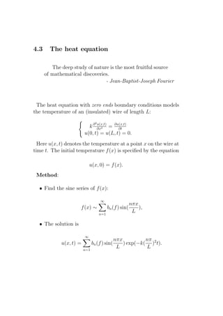
192. Example: Let
−1, 0 ≤ x ≤ π/2,
f (x) =
2, π/2 < x < π.
Then L = π and
π 1
2 2 cos(nπ) − 3 cos( 2 nπ) + 1
bn (f ) = f (x) sin(nx)dx = −2 .
π 0 nπ
Thus
2 6 2
f (x) ∼ b1 (f ) sin(x)+b2 (f ) sin(2x)+... = sin(x)− sin(2x)+ sin(3x)+....
π π 3π
This can also be done in SAGE :
SAGE
sage: f1 = lambda x: -1
sage: f2 = lambda x: 2
sage: f = Piecewise([[(0,pi/2),f1],[(pi/2,pi),f2]])
sage: P1 = f.plot()
sage: b10 = [f.sine_series_coefficient(n,pi) for n in range(1,10)]
sage: b10
[2/pi, -6/pi, 2/(3*pi), 0, 2/(5*pi), -2/pi, 2/(7*pi), 0, 2/(9*pi)]
sage: ss10 = sum([b10[n]*sin((n+1)*x) for n in range(len(b50))])
sage: ss10
2*sin(9*x)/(9*pi) + 2*sin(7*x)/(7*pi) - 2*sin(6*x)/pi
+ 2*sin(5*x)/(5*pi) + 2*sin(3*x)/(3*pi) - 6*sin(2*x)/pi + 2*sin(x)/pi
sage: b50 = [f.sine_series_coefficient(n,pi) for n in range(1,50)]
sage: ss50 = sum([b50[n]*sin((n+1)*x) for n in range(len(b))])
sage: P2 = ss10.plot(-5,5,linestyle="--")
sage: P3 = ss50.plot(-5,5,linestyle=":")
sage: (P1+P2+P3).show()
This illustrates how the series converges to the function. The
function f (x), and some of the partial sums of its sine series,
looks like Figure 4.6.

193. Figure 4.6: f (x) and two sine series approximations.
As you can see, taking more and more terms gives functions
which better and better approximate f (x).
The solution to the heat equation, therefore, is
∞
nπx nπ
u(x, t) = bn (f ) sin( ) exp(−k( )2 t).
n=1
L L
Next, we see how SAGE can plot the solution to the heat equa-
tion (we use k = 1):
SAGE
sage: t = var("t")
sage: soln50 = sum([b[n]*sin((n+1)*x)*eˆ(-(n+1)ˆ2*t) for n in range(len(b50))])
sage: soln50a = sum([b[n]*sin((n+1)*x)*eˆ(-(n+1)ˆ2*(1/10)) for n in range(len(b50))])
sage: P4 = soln50a.plot(0,pi,linestyle=":")

194. sage: soln50b = sum([b[n]*sin((n+1)*x)*eˆ(-(n+1)ˆ2*(1/2)) for n in range(len(b50))])
sage: P5 = soln50b.plot(0,pi)
sage: soln50c = sum([b[n]*sin((n+1)*x)*eˆ(-(n+1)ˆ2*(1/1)) for n in range(len(b50))])
sage: P6 = soln50c.plot(0,pi,linestyle="--")
sage: (P1+P4+P5+P6).show()
Taking 50 terms of this series, the graph of the solution at
t = 0, t = 0.5, t = 1, looks approximately like Figure 4.7.
Figure 4.7: f (x), u(x, 0.1), u(x, 0.5), u(x, 1.0) using 60 terms of the sine
series.
The heat equation with insulated ends boundary conditions
models the temperature of an (insulated) wire of length L:

195. 2
k ∂ ∂x2 = ∂u(x,t)
u(x,t)
∂t
ux (0, t) = ux (L, t) = 0.
Here ux (x, t) denotes the partial derivative of the temperature
at a point x on the wire at time t. The initial temperature f (x)
is specified by the equation u(x, 0) = f (x).
Method:
• Find the cosine series of f (x):
∞
a0 nπx
f (x) ∼ + an (f ) cos( ),
2 n=1
L
• The solution is
∞
a0 nπx nπ
u(x, t) = + an (f ) cos( )) exp(−k( )2 t).
2 n=1
L L
Example:
Let
−1, 0 ≤ x ≤ π/2,
f (x) =
2, π/2 < x < π.
Then L = π and
1
2 π sin 2 π n
an (f ) = f (x) cos(nx)dx = −6 ,
π 0 πn
for n > 0 and a0 = 1.
Thus

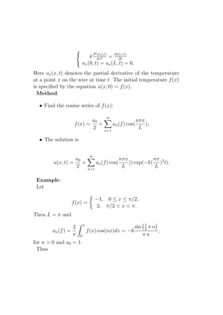
196. a0
+ a1 (f ) cos(x) + a2 (f ) cos(2x) + ...
f (x) ∼
2
This can also be done in SAGE :
SAGE
sage: f1 = lambda x: -1
sage: f2 = lambda x: 2
sage: f = Piecewise([[(0,pi/2),f1],[(pi/2,pi),f2]])
sage: P1 = f.plot()
sage: a10 = [f.cosine_series_coefficient(n,pi) for n in range(10)]
sage: a10
[1, -6/pi, 0, 2/pi, 0, -6/(5*pi), 0, 6/(7*pi), 0, -2/(3*pi)]
sage: a50 = [f.cosine_series_coefficient(n,pi) for n in range(50)]
sage: cs10 = a10[0]/2 + sum([a10[n]*cos(n*x) for n in range(1,len(a10))])
sage: P2 = cs10.plot(-5,5,linestyle="--")
sage: cs50 = a50[0]/2 + sum([a50[n]*cos(n*x) for n in range(1,len(a50))])
sage: P3 = cs50.plot(-5,5,linestyle=":")
sage: (P1+P2+P3).show()
This illustrates how the series converges to the function. The
piecewise constant function f (x), and some of the partial sums
of its cosine series (one using 10 terms and one using 50 terms),
looks like Figure 4.8.
As you can see, taking more and more terms gives functions
which better and better approximate f (x).
The solution to the heat equation, therefore, is
∞
a0 nπx nπ
u(x, t) = + an (f ) cos( ) exp(−k( )2 t).
2 n=1
L L
Using SAGE , we can plot this function:
SAGE
sage: soln50a = a50[0]/2 + sum([a50[n]*cos(n*x)*eˆ(-(n+1)ˆ2*(1/100)) for n in range(1,len(a50))])
sage: soln50b = a50[0]/2 + sum([a50[n]*cos(n*x)*eˆ(-(n+1)ˆ2*(1/10)) for n in range(1,len(a50))])
sage: soln50c = a50[0]/2 + sum([a50[n]*cos(n*x)*eˆ(-(n+1)ˆ2*(1/2)) for n in range(1,len(a50))])
sage: P4 = soln50a.plot(0,pi)
sage: P5 = soln50b.plot(0,pi,linestyle=":")

197. Figure 4.8: f (x) and two cosine series approximations.
sage: P6 = soln50c.plot(0,pi,linestyle="--")
sage: (P1+P4+P5+P6).show()
Taking only the first 50 terms of this series, the graph of the
solution at t = 0, t = 0.01, t = 0.1,, t = 0.5, looks approximately
like:

198. Figure 4.9: f (x) = u(x, 0), u(x, 0.01), u(x, 0.1), u(x, 0.5) using 50 terms of
the cosine series.
Explanation:
Where does this solution come from? It comes from the method
of separation of variables and the superposition principle. Here
is a short explanation. We shall only discuss the “zero ends”
case (the “insulated ends” case is similar).
2
First, assume the solution to the PDE k ∂ ∂x2 = ∂u(x,t) has the
u(x,t)
∂t
“factored” form
u(x, t) = X(x)T (t),
for some (unknown) functions X, T . If this function solves the

199. PDE then it must satisfy kX ′′ (x)T (t) = X(x)T ′ (t), or
X ′′ (x) 1 T ′ (t)
= .
X(x) k T (t)
Since x, t are independent variables, these quotients must be
constant. In other words, there must be a constant C such that
T ′ (t)
= kC, X ′′ (x) − CX(x) = 0.
T (t)
Now we have reduced the problem of solving the one PDE to
two ODEs (which is good), but with the price that we have
introduced a constant which we don’t know, namely C (which
maybe isn’t so good). The first ODE is easy to solve:
T (t) = A1 ekCt ,
for some constant A1 . To obtain physically meaningful solu-
tions, we do not want the temperature of the wire to become
unbounded as time increased (otherwise, the wire would simply
melt eventually). Therefore, we may assume here that C ≤ 0.
It is best to analyse two cases now:
Case C = 0: This implies X(x) = A2 +A3 x, for some constants
A2 , A3 . Therefore
a0
u(x, t) = A1 (A2 + A3 x) = + b0 x,
2
where (for reasons explained later) A1 A2 has been renamed a0
2
and A1 A3 has been renamed b0 .
Case C < 0: Write (for convenience) C = −r2 , for some r > 0.
The ODE for X implies X(x) = A2 cos(rx) + A3 sin(rx), for
some constants A2 , A3 . Therefore

200. 2 2
u(x, t) = A1 e−kr t (A2 cos(rx)+A3 sin(rx)) = (a cos(rx)+b sin(rx))e−kr t ,
where A1 A2 has been renamed a and A1 A3 has been renamed b.
These are the solutions of the heat equation which can be writ-
ten in factored form. By superposition, “the general solution”
is a sum of these:
+ b0 x + ∞ (an cos(rn x) + bn sin(rn x))e−krn t
a0 2
u(x, t) = 2 n=1
a0 2
= 2 + b0 x + (a1 cos(r1 x) + b1 sin(r1 x))e−kr1 t
2
+(a2 cos(r2 x) + b2 sin(r2 x))e−kr2 t + ...,
(4.5)
for some ai , bi , ri . We may order the ri ’s to be strictly increasing
if we like.
We have not yet used the IC u(x, 0) = f (x) or the BCs u(0, t) =
u(L, t) = 0. We do that next.
What do the BCs tell us? Plugging in x = 0 into (4.5) gives
∞
a0 2 a0 2 2
0 = u(0, t) = + an e−krn t = + a1 e−kr1 t + a2 e−kr2 t + ... .
2 n=1
2
These exponential functions are linearly independent, so a0 = 0,
a1 = 0, a2 = 0, ... . This implies
2 2 2
u(x, t) = b0 x+ bn sin(rn x)e−krn t = b0 x+b1 sin(r1 x)e−kr1 t +b2 sin(r2 x)e−kr2 t +
n=1
Plugging in x = L into this gives
2
0 = u(L, t) = b0 L + bn sin(rn L)e−krn t .
n=1

201. Again, exponential functions are linearly independent, so b0 = 0,
bn sin(rn L) for n = 1, 2, .... In other to get a non-trivial solution
to the PDE, we don’t want bn = 0, so sin(rn L) = 0. This forces
rn L to be a multiple of π, say rn = nπ/L. This gives
∞
nπ nπ 2 π π 2 2π 2π 2
u(x, t) = x)e−k( L ) t = b1 sin( x))e−k( L ) t +b2 sin( x))e−k( L ) t +...,
bn sin(
n=1
L L L
(4.6)
for some bi ’s. The special case t = 0 is the so-called “sine series”
expansion of the initial temperature function u(x, 0). This was
discovered by Fourier. To solve the heat eqution, it remains to
solve for the “sine series coefficients” bi .
There is one remaining condition which our solution u(x, t)
must satisfy.
What does the IC tell us? Plugging t = 0 into (4.6) gives
∞
nπ π 2π
f (x) = u(x, 0) = bn sin( x) = b1 sin( x))+b2 sin( x))+... .
n=1
L L L
In other words, if f (x) is given as a sum of these sine functions,
or if we can somehow express f (x) as a sum of sine functions,
then we can solve the heat equation. In fact there is a formula5
for these coefficients bn :
2 L nπ
bn = f (x) cos( x)dx.
L 0 L
It is this formula which is used in the solutions above.
Exercise: Solve the heat equation
5
Fourier did not know this formula at the time; it was discovered later by Dirichlet.

202. 2
2 ∂ ∂x2 = ∂u(x,t)
u(x,t)

 ∂t
ux (0, t) = ux (3, t) = 0
u(x, 0) = x,

using SAGE to plot approximations as above.

203. 4.4 The wave equation in one dimension
The theory of the vibrating string touches on musical theory
and the theory of oscillating waves, so has likely been a concern
of scholars since ancient times. Nevertheless, it wasn’t until
the late 1700s that mathematical progress was made. Though
the problem of describing mathematically a vibrating string re-
quires no calculus, the solution does. With the advent of cal-
culus, Jean le Rond dAlembert, Daniel Bernoulli, Leonard Eu-
ler, Joseph-Louis Lagrange were able to arrive at solutions to
the one-dimensional wave equation in the eighteenth-century.
Daniel Bernoulli’s solution dealt with an infinite series of sines
and cosines (derived from what we now call a “Fourier series”,
though it predates it), his contemporaries did not believe that
he was correct. Bernoullis technique would be later used by
Joseph Fourier when he solved the thermodynamic heat equa-
tion in 1807. It is Bernoulli’s idea which we discuss here as well.
Euler was wrong: Bernoulli’s method was basically correct after
all.
Now, d’Alembert was mentioned in the lecture on the trans-
port equation and it is worthwhile very briefly discussing what
his basic idea was. The theorem of dAlembert on the solution
to the wave equation is stated roughly as follows: The partial
differential equation:
∂ 2w ∂ 2w
= c2 ·
∂t2 ∂x2
is satisfied by any function of the form w = w(x, t) = g(x +
ct) + h(x − ct), where g and h are “arbitrary” functions. (This is
called “the dAlembert solution”.) Geometrically speaking, the

204. idea of the proof is to observe that ∂w ± c ∂w is a constant times
∂t ∂x
the directional derivative Dv± w(x, t), where v± is a unit vector
in the direction ±c, 1 . Therefore, you integrate
∂ 2w ∂ 2w
Dv− Dv+ w(x, t) = (const.) − c2 · =0
∂t2 ∂x2
twice, once in the v+ direction, once in the v− , to get the solu-
tion. Easier said than done, but still, that’s the idea.
The wave equation with zero ends boundary conditions models
the motion of a (perfectly elastic) guitar string of length L:
2 2
c2 ∂ w(x,t) = ∂ w(x,t)
∂x2 ∂t2
w(0, t) = w(L, t) = 0.
Here w(x, t) denotes the displacement from rest of a point x on
the string at time t. The initial displacement f (x) and initial
velocity g(x) at specified by the equations
w(x, 0) = f (x), wt (x, 0) = g(x).
Method:
• Find the sine series of f (x) and g(x):
∞ ∞
nπx nπx
f (x) ∼ bn (f ) sin( ), g(x) ∼ bn (g) sin( ).
n=1
L n=1
L
• The solution is
∞
nπt Lbn (g) nπt nπx
w(x, t) = (bn (f ) cos(c )+ sin(c )) sin( ).
n=1
L cnπ L L

205. Example: Let
−1, 0 ≤ t ≤ π/2,
f (x) =
2, π/2 < t < π,
and let g(x) = 0. Then L = π, bn (g) = 0, and
π
2 2 cos(nπ) − 3 cos(1/2 nπ) + 1
bn (f ) = f (x) sin(nx)dx = −2 .
π 0 n
Thus
2 6 2
f (x) ∼ b1 (f ) sin(x)+b2 (f ) sin(2x)+... = sin(x)− sin(2x)+ sin(3x)+....
π π 3π
The function f (x), and some of the partial sums of its sine series,
looks like
Figure 4.10: Using 50 terms of the sine series of f (x).
This was computed using the following SAGE commands:
SAGE
sage: x = var("x")
sage: f1 = lambda x: -1
sage: f2 = lambda x: 2

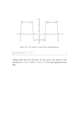
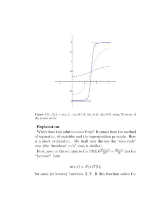
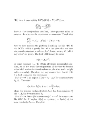
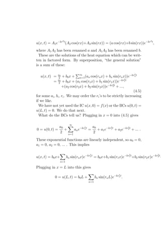
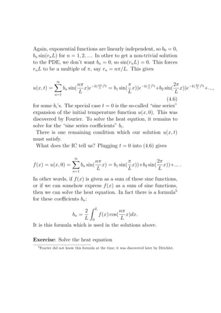
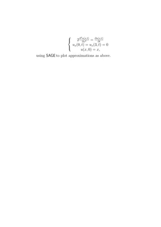
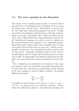
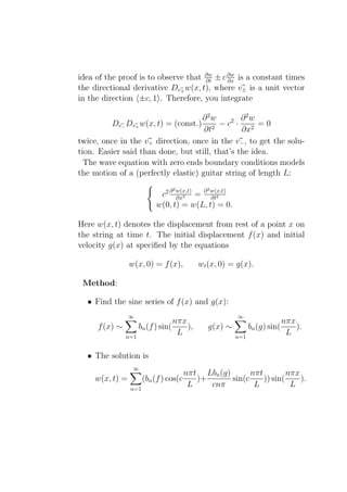
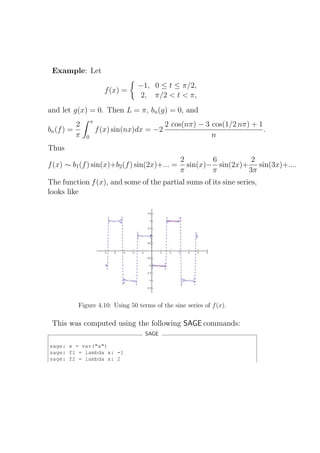
206. sage: f = Piecewise([[(0,pi/2),f1],[(pi/2,pi),f2]])
sage: P1 = f.plot(rgbcolor=(1,0,0))
sage: b50 = [f.sine_series_coefficient(n,pi) for n in range(1,50)]
sage: ss50 = sum([b50[i-1]*sin(i*x) for i in range(1,50)])
sage: b50[0:5]
[2/pi, -6/pi, 2/(3*pi), 0, 2/(5*pi)]
sage: P2 = ss50.plot(-5,5,linestyle="--")
sage: (P1+P2).show()
As you can see, taking more and more terms gives functions
which better and better approximate f (x).
The solution to the wave equation, therefore, is
∞
nπt Lbn (g) nπt nπx
w(x, t) = (bn (f ) cos(c )+ sin(c )) sin( ).
n=1
L cnπ L L
Taking only the first 50 terms of this series, the graph of the
solution at t = 0, t = 0.1, t = 1/5, t = 1/4, looks approximately
like:
Figure 4.11: Wave equation with c = 3.
This was produced using the SAGE commands:

207. SAGE
sage: t = var("t")
sage: w50t1 = sum([b50[i-1]*sin(i*x)*cos(3*i*(1/10)) for i in range(1,50)])
sage: P3 = w50t1.plot(0,pi,linestyle=":")
sage: w50t2 = sum([b50[i-1]*sin(i*x)*cos(3*i*(1/5)) for i in range(1,50)])
sage: P4 = w50t2.plot(0,pi,linestyle=":",rgbcolor=(0,1,0))
sage: w50t3 = sum([b50[i-1]*sin(i*x)*cos(3*i*(1/4)) for i in range(1,50)])
sage: P5 = w50t3.plot(0,pi,linestyle=":",rgbcolor=(1/3,1/3,1/3))
sage: (P1+P2+P3+P4+P5).show()
Of course, taking terms would give a better approximation to
w(x, t). Taking the first 100 terms of this series (but with dif-
ferent times):
Figure 4.12: Wave equation with c = 3.

208. Exercise: Solve the wave equation

 2 ∂ 2 w(x,t) = ∂ 2 w(x,t)

 ∂x2 ∂t2
w(0, t) = w(3, t) = 0


 w(x, 0) = x

 wt (x, 0) = 0,
using SAGE to plot approximations as above.

209. Bibliography
[A-pde] Wikipedia articles on the Transport equation:
http://en.wikipedia.org/wiki/Advection
http://en.wikipedia.org/wiki/Advection_equation
[A-uc] Wikipedia entry for the annihilator method: http://en.
wikipedia.org/wiki/Annihilator_method
[B-rref] Robert A. Beezer, A First Course in Linear Alge-
bra, released under the GNU Free Documentation License,
available at http://linear.ups.edu/
[B-ps] Wikipedia entry for the Bessel functions:
http://en.wikipedia.org/wiki/Bessel_function
[B-fs] Wikipedia entry for Daniel Bernoulli:
http://en.wikipedia.org/wiki/Daniel_Bernoulli
[BD-intro] W. Boyce and R. DiPrima, Elementary Differen-
tial Equations and Boundary Value Problems, 8th
edition, John Wiley and Sons, 2005.
[BS-intro] General wikipedia introduction to the Black-Scholes
model:
http://en.wikipedia.org/wiki/Black-Scholes
[C-ivp] General wikipedia introduction to the Catenary:
http://en.wikipedia.org/wiki/Catenary
201

210. [C-linear] General wikipedia introduction to RLC circuits:
http://en.wikipedia.org/wiki/RLC_circuit
[CS-rref] Wikipedia article on normal modes of coupled springs:
http://en.wikipedia.org/wiki/Normal_mode
[D-df] Wikipedia introduction to direction fields:
http://en.wikipedia.org/wiki/Slope_field
[DF-df] Direction Field Plotter of Prof Robert Israel:
http://www.math.ubc.ca/~israel/applet/dfplotter/
dfplotter.html
[D-spr] Wikipedia entry for damped motion: http://en.
wikipedia.org/wiki/Damping
[E-num] General wikipedia introduction to Euler’s method:
http://en.wikipedia.org/wiki/Euler_integration
[Eu1-num] Wikipedia entry for Euler: http://en.wikipedia.
org/wiki/Euler
[Eu2-num] MacTutor entry for Euler:
http://www-groups.dcs.st-and.ac.uk/~history/Biographies/Euler.html
[F-1st] General wikipedia introduction to First order linear
differential equations:
http://en.wikipedia.org/wiki/Linear_
differential_equation#First_order_equation
[F1-fs] Wikipedia Fourier series article
http://en.wikipedia.org/wiki/Fourier_series
[F2-fs] MacTutor Fourier biography:
http://www-groups.dcs.st-and.ac.uk/%7Ehistory/
Biographies/Fourier.html

211. [H-rref] Jim Hefferon, Linear Algebra, released under the
GNU Free Documentation License, available at http://
joshua.smcvt.edu/linearalgebra/
[H-ivp] General wikipedia introduction to the Hyperbolic trig
function
http://en.wikipedia.org/wiki/Hyperbolic_function
[H-intro] General wikipedia introduction to Hooke’s Law: http:
//en.wikipedia.org/wiki/Hookes_law
[H-fs] General wikipedia introduction to the heat equation:
http://en.wikipedia.org/wiki/Heat_equation
[H1-spr] Wikipedia entry for Robert Hooke: http://en.
wikipedia.org/wiki/Robert_Hooke
[H2-spr] MacTutor entry for Hooke:
http://www-groups.dcs.st-and.ac.uk/%7Ehistory/Biographies/Hooke.html
[KL-cir] Wikipedia entry for Kirchhoff’s laws: http://en.
wikipedia.org/wiki/Kirchhoffs_circuit_laws
[K-cir] Wikipedia entry for Kirchhoff: http://en.wikipedia.
org/wiki/Gustav_Kirchhoff
[L-var] Wikipedia article on Joseph Louis Lagrange:
http://en.wikipedia.org/wiki/Joseph_Louis_
Lagrange
[LE-sys] Everything2 entry for Lanchester’s equations:
http://www.everything2.com/index.pl?node=
Lanchester%20Systems%20and%20the%20Lanchester%
20Laws%20of%20Combat

212. [L-sys] Wikipedia entry for Lanchester: http://en.
wikipedia.org/wiki/Frederick_William_Lanchester
[LA-sys] Lanchester automobile information: http:
//www.amwmag.com/L/Lanchester_World/lanchester_
world.html
[L-intro] F. W. Lanchester, Mathematics in Warfare, in The
World of Mathematics, J. Newman ed., vol.4, 2138-
2157, Simon and Schuster (New York) 1956; now Dover
2000. (A four-volume collection of articles.)
http://en.wikipedia.org/wiki/Frederick_W.
_Lanchester
[La-sys] Frederick William Lanchester, Aviation in Warfare:
The Dawn of the Fourth Arm, Constable and Co., Lon-
don, 1916.
[L-lt] Wikipedia entry for Laplace: http://en.wikipedia.
org/wiki/Pierre-Simon_Laplace
[LT-lt] Wikipedia entry for Laplace transform: http://en.
wikipedia.org/wiki/Laplace_transform
[L-linear] General wikipedia introduction to Linear Indepen-
dence:
http://en.wikipedia.org/wiki/Linearly_
independent
[Lo-intro] General wikipedia introduction to the logistic func-
tion model of population growth:
http://en.wikipedia.org/wiki/Logistic_function
[M-intro] Niall J. MacKay, Lanchester combat models, May
2005. http://arxiv.org/abs/math.HO/0606300

213. [M-ps] Sean Mauch, Introduction to methods of Applied Mathe-
matics,
http://www.its.caltech.edu/~sean/book/
unabridged.html
[M] Maxima, a general purpose Computer Algebra system.
http://maxima.sourceforge.net/
[M-mech] General wikipedia introduction to Newtonian me-
chanics
http://en.wikipedia.org/wiki/Classical_mechanics
[M-fs] Wikipedia entry for the physics of music:
http://en.wikipedia.org/wiki/Physics_of_music
[N-mech] General wikipedia introduction to Newton’s three
laws of motion:
http://en.wikipedia.org/wiki/Newtons_Laws_of_
Motion
[N-intro] David H. Nash, Differential equations and the Battle of
Trafalgar, The College Mathematics Journal, Vol. 16, No.
2 (Mar., 1985), pp. 98-102.
[N-cir] Wikipedia entry for Electrical Networks: http://en.
wikipedia.org/wiki/Electrical_network
[NS-intro] General wikipedia introduction to Navier-Stokes
equations:
http://en.wikipedia.org/wiki/Navier-Stokes_
equations
Clay Math Institute prize page:
http://www.claymath.org/millennium/
Navier-Stokes_Equations/

214. [O-ivp] General wikipedia introduction to the Harmonic oscilla-
tor
http://en.wikipedia.org/wiki/Harmonic_oscillator
[P-fs] Howard L. Penn, “Computer Graphics for the Vibrating
String,” The College Mathematics Journal, Vol. 17, No. 1
(Jan., 1986), pp. 79-89
[P1-ps] Wikipedia entry for Power series: http://en.
wikipedia.org/wiki/Power_series
[P2-ps] Wikipedia entry for the power series method: http:
//en.wikipedia.org/wiki/Power_series_method
[R-ps] Wikipedia entry for the recurrence relations:
http://en.wikipedia.org/wiki/Recurrence_
relations
[R-cir] General wikipedia introduction to LRC circuits: http:
//en.wikipedia.org/wiki/RLC_circuit
[S-intro] The SAGE Group, SAGE : Mathematical software, ver-
sion 2.8.
http://www.sagemath.org/
http://sage.scipy.org/
[SH-spr] Wikipedia entry for Simple harmonic motion: http:
//en.wikipedia.org/wiki/Simple_harmonic_motion
[S-pde] W. Strauss, Partial differential equations, an introduc-
tion, John Wiley, 1992.
[U-uc] General wikipedia introduction to undetermined co-
efficients: http://en.wikipedia.org/wiki/Method_of_
undetermined_coefficients

215. [V-var] Wikipedia introduction to variation of parameters:
http://en.wikipedia.org/wiki/Method_of_
variation_of_parameters
[W-intro] General wikipedia introduction to the Wave equation:
http://en.wikipedia.org/wiki/Wave_equation
[W-mech] General wikipedia introduction to Wile E. Coyote
and the RoadRunner:
http://en.wikipedia.org/wiki/Wile_E._Coyote_and_
Road_Runner
[W-linear] General wikipedia introduction to the Wronskian
http://en.wikipedia.org/wiki/Wronskian
[Wr-linear] St. Andrews MacTutor entry for Wronski
http://www-groups.dcs.st-and.ac.uk/%7Ehistory/Biographies/Wronski.
html