Constant Voltage Transformer Design

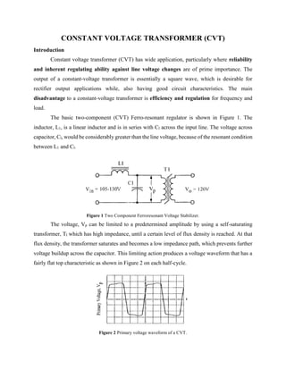
1. CONSTANT VOLTAGE TRANSFORMER (CVT)
Introduction
Constant voltage transformer (CVT) has wide application, particularly where reliability
and inherent regulating ability against line voltage changes are of prime importance. The
output of a constant-voltage transformer is essentially a square wave, which is desirable for
rectifier output applications while, also having good circuit characteristics. The main
disadvantage to a constant-voltage transformer is efficiency and regulation for frequency and
load.
The basic two-component (CVT) Ferro-resonant regulator is shown in Figure 1. The
inductor, L1, is a linear inductor and is in series with Cl across the input line. The voltage across
capacitor, Cl, would be considerably greater than the line voltage, because of the resonant condition
between L1 and Cl.
Figure 1 Two Component Ferroresonant Voltage Stabilizer.
The voltage, Vp can be limited to a predetermined amplitude by using a self-saturating
transformer, Tl which has high impedance, until a certain level of flux density is reached. At that
flux density, the transformer saturates and becomes a low impedance path, which prevents further
voltage buildup across the capacitor. This limiting action produces a voltage waveform that has a
fairly flat top characteristic as shown in Figure 2 on each half-cycle.
Figure 2 Primary voltage waveform of a CVT.

2. Electrical Parameters of a CVT Line Regulator
When the constant voltage transformer is operating as a line regulator, the output voltage
will vary as a function of the input voltage, as shown in Figure 3. The magnetic material used to
design transformer, Tl, has an impact on line regulation. Transformers designed with a square B-
H loop will result in better line regulation. If the output of the line regulator is subjected to a load
power factor (lagging) with less than unity, the output will change, as shown in Figure 4.
Figure 3 Output Voltage Variation as a function of input voltage.
Figure 4 Output voltage variation as a function of load power factor.
If the constant voltage transformer is subjected to a line voltage frequency change the
output voltage will vary, as shown in Figure 5. Capability for handling short circuit is an inherent
feature of a constant-voltage transformer. The short-circuit current is limited and set by the series
inductance L. The regulation characteristics at various lines and loads are shown in Figure 6. It

3. should be noted that a dead short, corresponding to zero output voltage, does not greatly increase
the load current; whereas for most transformers, this dead short would be destructive.
Figure 5 Output voltage variation as a function of line frequency change.
Figure 6 Output voltage variation as a function of output voltage vs. load.
Constant Voltage Transformer, Design Equations
Proper operation and power capacity of a constant-voltage transformer (CVT) depends on
components, L1 and Cl, as shown in Figure 7. Experience has shown that the, LC, relationship is:
5.12
LC (1)
2
)(0 RR
L  (2)
)(033.0
1
RR
C

 (3)

4. Figure 7 Basic constant voltage circuit.
Referring to Figure 11-7, assume there is a sinusoidal input voltage, an ideal input inductor,
L1, and a series capacitor, Cl. RO(R), is the reflected resistance back to the primary, including
efficiency.  is the efficiency and P0, is the output power.
0
2
0
R
V
P s
 (4)
Input power,
)(0
2
0
R
P
in
R
VP
P 

(5)
0
2
)(0
P
V
R
p
R

 (6)
It is common practice for the output to be isolated from the input and to connect Cl to a
step-up winding on the constant-voltage transformer (CVT). In order to use smaller capacitor
values, a step-up winding must be added, as shown in Figure 8. The penalty for using a smaller
capacitor requires the use of a step up winding. This step-up winding increases the VA or size of
the transformer.
Figure 8 CVT with step-up winding.

5. The secondary current, Is, can be expressed as:
s
s
V
P
I 0
 (7)
With the step-up winding, the primary current Ip is related to the secondary current by
equation:
 
  












)31(
)21(
)21(
)54(
1
C
P
P
SS
P
V
V
V
VI
I

(8)
Due to increase in odd harmonics (because of saturation), current through the capacitor is
increased by a factor Kc, so capacitor current is given by:
CVKI CCC  (9)
Where Kc can vary from 1.0 to 1.5.
Empirically, it has been seen that for good performance the primary operating voltage
should be:
)95.0(inP VV  (10)
When the resonating capacitor is connected across a step-up winding, as is Figure 8, both
the value of the capacitor and the volume get reduced. If Cn is the new capacitance value and Vn
is the new voltage across the capacitor then
2
)21()21(
2
 VCVC nn (11)
The apparent power Pt is the sum of each winding VA, i.e.
)54()32()21(   VAVAVAPt (12)
Design a constant voltage transformer with the following specifications:
i. Input voltage Vin= 200-250 V
ii. Output voltage Vs = 230 V
iii. Power rating Po= 250 VA (Watts)
Engineering specifications: -
i. Supply frequency f = 50 Hz
ii. Current density J = 300 A/m2
iii. Capacitor voltage VC = 440 Volts
iv. Capacitor coefficient Kc = 1.5
v. Efficiency  = 85 %

6. vi. Saturating flux density Bs = 1.95 T
vii. Window utilization factor Ku = 0.4.
Design steps: -
Step 1: - Calculation of primary voltage.
Primary voltage,
VoltsVV inP 19095.020095.0(min)  .
Step 2: - Calculation of reflected resistance back to primary.
Reflected load resistance back to primary,




 74.122
250
85.01902
0
2
)(
P
V
R P
RO

.
Step 3: - Calculation of required resonating capacitance.
Value of required resonating capacitance,
.59.78
74.12250233.0
1
33.0
1
)(
F
Rw
C
RO







Step 4: - Calculation of new value of capacitance with step-up winding.
New value of capacitance with step-up winding,
.655.14
440
19059.78
2
2
2
)31(
2
)21(
)31( F
V
VC
C 







Generally VF 440/15 capacitors are available in market, so it is selected for CVT
operation.
Step 5: - Calculation of current through the capacitor.
Current through the capacitor,
AmpCwVI Cc 11.310155024405.15.1 6
 
 .
Step 6: - Calculation of secondary current.
Secondary current,
Amp
V
P
I
S
S 087.1
230
2500
 .

7. Step 7: - Calculation of primary current.
Primary current,
Amp
V
V
V
VI
I
C
P
P
SS
P 565.2
440
190
1
19085.0
230087.1
1
)31(
)21(
)21(
)54(




























.
Step 8: - Calculation of total power handling capability.
Total power handling capability,
VA
IVIVVIV
VAVAVAP
SSCPCPP
t
86.1514087.123011.3)190440(565.2190
)(
)54()32()21(


 
Step 9: - Calculation the area product.
Area product,
4
44
28.299
3009.1504.044.4
1086.151410
cm
JfBKK
P
A
Suf
t
p 




 .
Step 10: - Selection of Core.
The closest lamination to the calculated area product in previous step is EI-175.
Table 1: Design data for various EI laminations.

8. Table 2: Dimensional data for various EI laminations.
E
D
D
Figure 3 Outline of EI laminations.
For EI-175 Lamination
Mean length turn MLT = 25.6 cm.
Magnetic path length MPL = 27.7 cm.
Core area Ac = 18.77 cm2
.
Window area Wa = 14.818 cm2
.
Area product Ap = 278.145 cm4
.
Core geometry Kg = 81.656 cm5
.
Surface area At = 652 cm2
.
Core weight Wtfe = 3.71 Kg.
Step 11: - Calculation of number of primary turns.
Number of primary turns,
23483.233
77.18509.144.4
1019010 44






cSf
p
p
fABK
V
N turns.

9. Step 12: - Calculation of primary bare conductor area.
Bare cross-sectional area of primary winding,
22
)( 855.000855.0
300
565.2
mmcm
J
I
A p
Bwp  .
Step 13: - Selection of wire for primary winding.
Cross-sectional area of the required wire close to the area calculated in step-12 is close to
that of SWG-19 conductor. So the selected wire for designing the inductor is SWG-19.
Table 3: Standard Wire Gauge table.
Standard Wire
Gauge (SWG)
Diameter
in mm
Cross-sectional
area in mm2
Resistance per length
in Ω/Km in µΩ/cm
18 1.22 1.17 14.8 148
19 1.02 0.811 21.3 213
20 0.914 0.657 26.3 263
For 19-SWG wire, bare conductor area if 0.811 mm2
and resistance is 213 cm/ .
Step 14: - Calculation of primary winding resistance.
Primary winding resistance,
 
276.1102132346.2510213 66
pp NMLTR
Step 15: - Calculation of Primary winding copper loss.
Primary winding copper loss,
WRIP ppp 4.8276.1565.2 22
 .
Step 16: - Calculation for number of turns for step-up capacitor winding.
Number of turns required for step-up capacitor winding,
30889.307
190
)190440(234)(





p
pcp
c
V
VVN
N turns.

10. Step 17: - Calculation of bare wire area for step-up capacitor winding.
Bare cross-sectional area of step-up capacitor winding,
22
)( 04.10104.0
300
11.3
mmcm
J
I
A C
Bwc  .
Step 18: - Selection of wire for step-up capacitor winding.
Cross-sectional area of the required wire close to the area calculated in step-17 is close to
that of SWG-18 conductor. So the selected wire for designing the inductor is SWG-18.
Table 3: Standard Wire Gauge table.
Standard Wire
Gauge (SWG)
Diameter
in mm
Cross-sectional
area in mm2
Resistance per length
in Ω/Km in µΩ/cm
17 1.42 1.59 10.9 109
18 1.22 1.17 14.8 148
19 1.02 0.811 21.3 213
For 18-SWG wire, bare conductor area if 1.17 mm2
and resistance is 148 cm/ .
Step 19: - Calculation of step-up capacitor winding resistance.
Step-up capacitor winding resistance,
 
167.1101483086.2510148 66
cc NMLTR
Step 20: - Calculation of step-up capacitor winding copper loss.
Step-up capacitor winding copper loss,
WRIP ssc 3.11167.111.3 22
 .
Step 21 - Calculation for number of turns for secondary winding.
Number of turns required for the secondary winding,
2843.283
190
230234





p
p
s
V
VsN
N turns.

11. Step 22: - Calculation of bare wire area for secondary winding.
Bare cross-sectional area of secondary winding,
22
)( 362.000362.0
300
087.1
mmcm
J
I
A s
Bws  .
Step 23: - Selection of wire for secondary winding.
Cross-sectional area of the required wire close to the area calculated in step-17 is close to
that of SWG-22 conductor. So the selected wire for designing the inductor is SWG-22.
Table 3: Standard Wire Gauge table.
Standard Wire
Gauge (SWG)
Diameter
in mm
Cross-sectional
area in mm2
Resistance per length
in Ω/Km in µΩ/cm
21 0.813 0.519 33.2 332
22 0.711 0.397 43.4 434
23 0.61 0.292 59.1 591
For 22-SWG wire, bare conductor area if 0.397 mm2
and resistance is 434 cm/ .
Step 24: - Calculation of secondary winding resistance.
Secondary winding resistance,
 
155.3104342846.2510434 66
sp NMLTR
Step 25: - Calculation of secondary winding copper loss.
Secondary winding copper loss,
WRIP sss 73.3155.3087.1 22
 .
Step 26: - Calculation of total copper loss.
Total copper loss,
WPcu 43.2373.33.114.8  .

12. Step 27: - Calculation of W/K for the core material.
38.195.150000557.0000557.0 86.168.186.168.1
 Bf
K
W
Step 28: - Calculation of core loss.
Core loss,
WWt
K
W
P fefe 12.571.338.1 
Step 29: - Calculation the total losses.
Total losses, WPPP fecu 57.2812.543.23  .
Step 30: - Calculation of watt density.
Surface watt density, 044.0
652
57.28
 
tA
P
 .
Step 31: - Calculation the temperature rise.
Temperature rise, .1.34044.0450450 0826.0826.0
CTr  
Step 32: - Calculation of transformer efficiency.
Transformer efficiency, %.74.898974.0
57.28250
250





PP
P
o
o

Step 33: - Window utilization factor.
454.0
6.14
0117.030800397.028400811.0234
)()()(





a
BwccBwssBwpp
u
W
ANANAN
K

13. Series AC Inductor Design
Voltage rating of the inductor is the highest input voltage i.e. 250V and current rating is
the input current is the primary current Ip i.e. 2.565 A. Various parameters considered for designing
inductor are:
Operating frequency: f = 50 Hz
Operating flux density: B = 1.4 T
Current density: J = 300 A/cm2
Efficiency: 85 %
Magnetic material permeability, r = 1500
Window utilization, Ku = 0.4
Step 34: - Calculation of inductance.
Inductive reactance,  466.97
565.2
250
LX .
Inductance, H
f
X
X L
L 31.0
502
466.97
2






Step 35: - Calculation of power handling capability.
Power handling capability of the inductor is
VAPt 25.641565.2250  .
Step 36:- Calculation of area product AP
4
44
94.171
3004.1504.044.4
1025.64110
cm
JfBKk
P
A
acuf
t
p 





Step 37:- Selection of Core
Core material suitable for designing the inductor is EI-150 for which the area product is
150.136 cm4
. Tables blow depicts the design and dimensional data for various laminations EI
(Table 3.3 of Text Book).

14. Table 1: Design data for various EI laminations.
Table 2: Dimensional data for various EI laminations.
E
D
D
Figure 3 Outline of EI laminations.
For 𝑬𝑰 − 𝟏𝟓𝟎 lamination,
Magnetic path length (MPL) = 22.9 cm
Core weight = 2.334 Kg
Copper weight = 853 gm

15. Mean length turn (MLT) = 22 cm
Iron area, 𝐴 𝑐 = 13.79 cm2
Window area, 𝑊𝑎 = 10.89 cm2
Area product, 𝐴 𝑝 = 𝐴 𝑐 × 𝑊𝑎 = 150.136 cm4
Core geometry, 𝐾𝑔 = 37.579 cm5
Surface area, 𝐴 𝑡 = 479 cm2
Window length, G = 5.715 cm
Lamination tongue, E = 3.81 cm
Step 38:- Calculation of number of turns
584
79.13504.144.4
1025010 44






cacf fABk
V
N turns.
Step 39:- Calculation of required air-gap
mmcm
MPL
L
AN
l
r
c
g 75.1175.0
1500
9.22
31.0
1079.135844.0104.0 8282















Step 40:- Calculation of Fringing flux factor
197.1
175.0
715.52
ln
79.13
175.0
1
2
ln1 




 










gc
g
l
G
A
l
F
Step 41:- Calculation of new number of turns for the inductor
512
10197.179.134.0
175.031.0
104.0 88





 
 FA
Ll
N
c
g
new turns.
Step 42:- Calculation of operating flux density with new turns
595.1
79.135051244.4
1025010 44






cnewf
ac
fANk
V
B T
Step 43:- Calculation of bare conductor area
22
)( 855.000855.0
300
565.2
mmcm
J
I
A Bw 
Step 44:- Selection of wire from wire table
Cross-sectional area of the required wire close to the area calculated in step-10 is matching
with the area of SWG-19 conductor. So the selected wire for designing the inductor is SWG-19.

16. Table 3: Standard Wire Gauge table.
Standard wire gauge Diameter in mm
Cross-sectional area in
mm2
Resistance per length
in Ω/Km in µΩ/cm
18 1.22 1.17 14.8 148
19 1.02 0.811 21.3 213
20 0.914 0.657 26.3 263
For 19-SWG wire, bare conductor area if 0.811 mm2
and resistance is 213 cm/ .
Step 45:- Calculation of inductor resistance
Inductor resistance,
 
4.2102135122210213 66
newL NMLTR
Step 46:- Inductor winding copper loss
79.154.2565.2 22
 LL RIP Watts
Step 47: - Calculation of Watts/Kg 





K
W
95.0595.150000557.0000557.0 86.168.186.168.1
 acBf
K
W
Step 48: - Calculation of core loss
22.2334.295.0  tfefe W
K
W
P Watts
Step 49: - Calculation of gap loss
146.13595.150175.081.3155.0 22
 acgig fBElKP Watts
Step 50: - Calculation of total losses
136.31146.132.279.15  gfecu PPPP Watts
Step 51: - Calculation inductor surface watt density
065.0
479
136.31
 
tA
P
 Watts/cm2
Step 52: - Calculation of temperature rise
CTr
0826.0826.0
5.40065.0400400  
Step 53:- Calculation of window utilization factor

17. 38.0
887.10
00811.0512





a
wBnew
u
w
AN
K