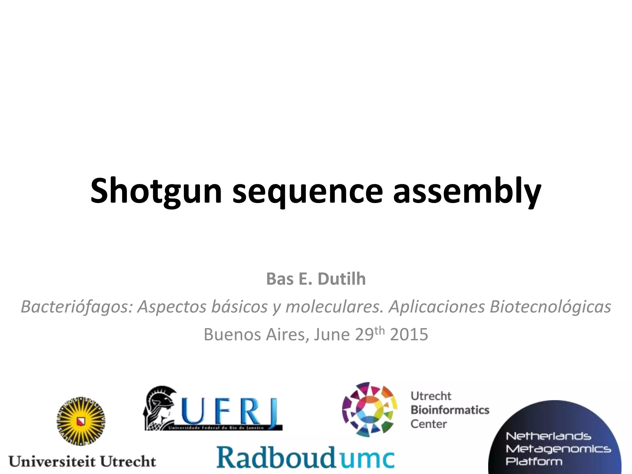
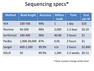
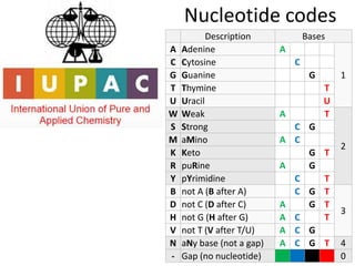
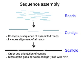
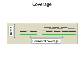
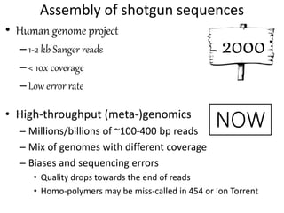
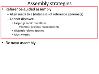
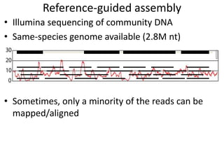
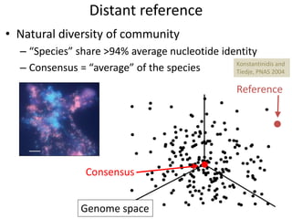
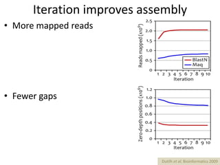
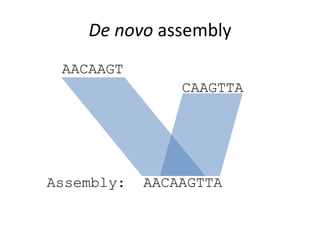
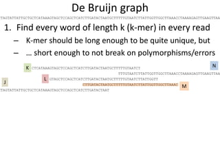
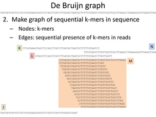
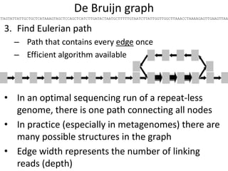
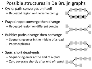
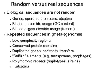
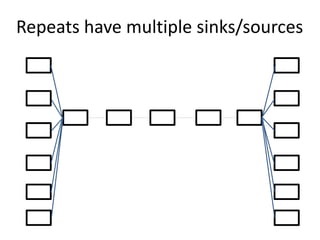
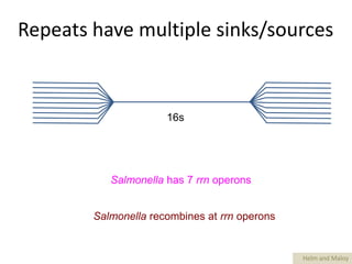
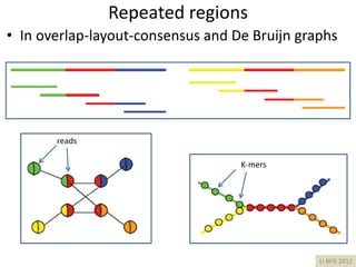
Metagenome Sequence Assembly (CABBIO 20150629 Buenos Aires)

Bas E. Dutilh
Bacteriófagos: Aspectos básicos y moleculares. Aplicaciones Biotecnológicas
Buenos Aires, June 29th 2015
Shotgun sequence assembly

Method Read length Accuracy Million
reads
Time Cost
per M
454 100-700 99% 1 1 day $10
Illumina 50-300 98% 3,000 1-2 days $0.10
IonTorrent 100-400 98% 40-80 2 hours $1
PacBio 1,000-30,000 87% 0.05 2 hours $1
Sanger 400-1,200 99.9% n/a 2 hours $2,400
SOLiD 50 99.9% 1,200 1-2 weeks $0.13
Sequencing specs*
* these numbers change all the time!

Lengths of reads and genomes
 NGS technologies provide reads of 50 to max.
30,000 bp, but most genomes are much longer
Gago, Science 2009

Nucleotide codes
Description Bases
A Adenine A
1
C Cytosine C
G Guanine G
T Thymine T
U Uracil U
W Weak A T
2
S Strong C G
M aMino A C
K Keto G T
R puRine A G
Y pYrimidine C T
B not A (B after A) C G T
3
D not C (D after C) A G T
H not G (H after G) A C T
V not T (V after T/U) A C G
N aNy base (not a gap) A C G T 4
- Gap (no nucleotide) 0

Sequence File Formats
• Different file formats for different uses
• Competing formats developed in parallel
• Some easy to read, some easy to parse

• Simplest sequence file format
• Unique identifiers!
• “Fasta wide” format has the whole sequence on one line
• Even easier to parse in a computer script
Fasta
>identifier1 [optional information]
CCGATCATATGACTAGCATGCATCGATCGATCGACTAGCATTT
AGAGCTACGATCAGCACTACACGCTTTGTATGATTGGCGGCGG
CTATTATATTGGGA
>identifier2 [optional information]
GAGAGCTACGATCAGAGCTACGATCAGCACTACACGCTTTGTA
TGATTGGCCCCCTATATTGGGACACGATCAGCACTACACGCTT
TGTATGATTGGCGGCGGCTATCCGATCAT

• Based on Fasta format
• Contains information about quality of each nucleotide
• Quality estimated by sequencing machine
@SRR014849.1 EIXKN4201CFU84 length=93
GGAAATGGAGTACGGATCGATTTTGTTTGGAACCGAAAGGGTC
+
hhhhhhhhhhhhhhhh7F@71,'";C?,B;?6B;:EA1EA1E%
• Four lines per sequence:
1. Identifier line starting with @
2. DNA sequence on one line
3. Second identifier line starting with + (identifier optional)
4. String of quality scores on one line
Fastq

Quality scores
 Phred 10: 10-1 chance that the base is wrong
 90% accuracy; 10% error rate
 99% accuracy ; 1% error rate
 99.9% accuracy ; 0.1% error rate
 Etcetera

ASCII character codes
 Fastq quality score: Phred score + 33, converted to
ASCII text
 Note: old Illumina format was different!
@SRR014849.1 EIXKN4201CFU84 length=93
GGAAATGGAGTACGGATCGATTTTGTTTGGAACCGAAAGGGTC
+
hhhhhhhhhhhhhhhh7F@71,'";C?,B;?6B;:EA1EA1E%

Quality profile of reads
March 2011

Quality profile of reads
October 2011

Random genome, random coverage
• Average depth:
– Genome size G
– Base depth B=40x
– Read length L=100 bp
– K-mer size K=25 bp
C = B * (L - K + 1) / L
• Uncovered bases:
u = G * eC
CTAGTATTATTGCTGCTCATAAAGTAGCTCCAGCTCATCTTGATACTAATGCTTTTTGTAATCTTATTGGTTGGCTTAAACCTAAAAGAGTTGAAGTTAA

What is easier to assemble?
Random sequences, or real genomes?

Sequence assembly
Reads
Scaffold
 Order and orientation of contigs
 Sizes of the gaps between contigs (filled with NNN)
Contigs
 Consensus sequence of assembled reads
 Includes alignment of all reads

Horizontal coverage
Depth
Coverage

Assembly of shotgun sequences
• Human genome project
–1-2 kb Sanger reads
–< 10x coverage
–Low error rate
• High-throughput (meta-)genomics
– Millions/billions of ~100-400 bp reads
– Mix of genomes with different coverage
– Biases and sequencing errors
• Quality drops towards the end of reads
• Homo-polymers may be miss-called in 454 or Ion Torrent
2000
NOW

Assembly strategies
• Reference-guided assembly
– Align reads to a (database) of reference genome(s)
– Cannot discover:
• Larger genomic mutations
– Insertions, deletions, rearrangements
• Distantly related species
• Most viruses
• De novo assembly
– Requires sufficient coverage x depth
– Breaks on repeats and low-coverage regions
– Algorithms
• Greedy assembly (only to illustrate)
• Overlap-layout-consensus
• De Bruijn graph

Reference-guided assembly
• Illumina sequencing of community DNA
• Same-species genome available (2.8M nt)
• Sometimes, only a minority of the reads can be
mapped/aligned

Distant reference
• Natural diversity of community
– “Species” share >94% average nucleotide identity
– Consensus = “average” of the species
Consensus
Genome space
Reference
Konstantinidis and
Tiedje, PNAS 2004

• The assembly is a better representation of the community
• Can we further approach the consensus genome by re-
mapping the reads against this first assembly?
Reference
Genome space
Iterative mapping and assembly
First assembly
Consensus
Dutilh et al. Bioinformatics 2009

Iteration improves assembly
• More mapped reads
• Fewer gaps
Dutilh et al. Bioinformatics 2009

De novo assembly
Assembly: AACAAGTTA
AACAAGT
CAAGTTA

De novo assembly approaches
• Greedy approach
• De Bruijn graphs

Greedy assembly
1. Sequences (reads)
2. Pairwise all-vs-all similarities
3. Find best matching pair
4. Collapse/assemble
• Works well for few, long reads (Sanger)
– All-vs-all calculations are expensive
– One clear best match
• Does not work for high throughput NGS datasets
– Many reads -> expensive to calculate
– Low coverage requires graph approach
(reads/contigs)

Repetitive sequences
• Reads A-D are from a region with two long repeats
• Greedy approach would first join A-D with the
largest overlap, and place B-C in a separate contig
• Resolving this requires a global view of all the
possibilities before joining two reads: a graph
repeat repeat
DA
C
B
D C
BA
B
D

Assembly as a “graph” problem
• De Bruijn Graph
• A graph contains nodes and edges
node edge

1. Identify all overlaps between reads
– Use cutoffs: minimum overlap and percent identity
2. Make graph of overlap connections
– Nodes: reads
– Edges: overlaps
3. Find Hamiltonian path
– Path that contains every node once
– No efficient algorithm available
4. Determine consensus at each position
TTTGTAATCTTATTGGTTGGCTTAAACCTAAAAGAGTTGAAGTTAA
Overlap-layout-consensus
CTAGTATTATTGCTGCTCATAAAGTAGCTCCAGCTCATCTTGATACTAAT
CTCATAAAGTAGCTCCAGCTCATCTTGATACTAATGCTTTTTGTAATCT
GTAGCTCCAGCTCATCTTGATACTAATGCTTTTTGTAATCTTATTGGTT
CTTGATACTAATGCTTTTTGTAATCTTATTGGTTGGCTTAAAC
K N
LJ
M
K NLJ M

De Bruijn graph
1. Find every word of length k (k-mer) in every read
– K-mer should be long enough to be quite unique, but
– … short enough to not break on polymorphisms/errors
CTTGATACTAATGCTTTTTGTAATCTTAT
TTGATACTAATGCTTTTTGTAATCTTATT
TGATACTAATGCTTTTTGTAATCTTATTG
GATACTAATGCTTTTTGTAATCTTATTGG
ATACTAATGCTTTTTGTAATCTTATTGGT
TACTAATGCTTTTTGTAATCTTATTGGTT
ACTAATGCTTTTTGTAATCTTATTGGTTG
CTAATGCTTTTTGTAATCTTATTGGTTGG
TAATGCTTTTTGTAATCTTATTGGTTGGC
AATGCTTTTTGTAATCTTATTGGTTGGCT
ATGCTTTTTGTAATCTTATTGGTTGGCTT
TGCTTTTTGTAATCTTATTGGTTGGCTTA
GCTTTTTGTAATCTTATTGGTTGGCTTAA
CTTTTTGTAATCTTATTGGTTGGCTTAAA
TTTTTGTAATCTTATTGGTTGGCTTAAAC
K N
L
M
J

De Bruijn graph
2. Make graph of sequential k-mers in sequence
– Nodes: k-mers
– Edges: sequential presence of k-mers in reads
CTTGATACTAATGCTTTTTGTAATCTTAT
TTGATACTAATGCTTTTTGTAATCTTATT
TGATACTAATGCTTTTTGTAATCTTATTG
GATACTAATGCTTTTTGTAATCTTATTGG
ATACTAATGCTTTTTGTAATCTTATTGGT
TACTAATGCTTTTTGTAATCTTATTGGTT
ACTAATGCTTTTTGTAATCTTATTGGTTG
CTAATGCTTTTTGTAATCTTATTGGTTGG
TAATGCTTTTTGTAATCTTATTGGTTGGC
AATGCTTTTTGTAATCTTATTGGTTGGCT
ATGCTTTTTGTAATCTTATTGGTTGGCTT
TGCTTTTTGTAATCTTATTGGTTGGCTTA
GCTTTTTGTAATCTTATTGGTTGGCTTAA
CTTTTTGTAATCTTATTGGTTGGCTTAAA
TTTTTGTAATCTTATTGGTTGGCTTAAAC
K N
L
J
M

De Bruijn graph
3. Find Eulerian path
– Path that contains every edge once
– Efficient algorithm available
• In an optimal sequencing run of a repeat-less
genome, there is one path connecting all nodes
• In practice (especially in metagenomes) there are
many possible structures in the graph
• Edge width represents the number of linking
reads (depth)

Possible structures in De Bruijn graphs
• Cycle: path converges on itself
– Repeated region on the same contig
• Frayed rope: converge then diverge
– Repeated region on different contigs
• Bubble: paths diverge then converge
– Sequencing error in the middle of a read
– Polymorphisms
• Spur: short dead-ends
– Sequencing error at the end of a read
– Zero coverage shortly after end of repeat

Examples of De Bruijn graphs
1% 5%
10% 15%
Pell PNAS 2012
Sequencing errors in a
random circular sequence
Peng Bioinformatics 2011
Five E. coli subspecies

Random versus real sequences
 Biological sequences are not random
 Genes, operons, promoters, etcetera
 Biased nucleotide usage (GC content)
 Biased oligonucleotide usage (k-mers)
 Repeated sequences in (meta-)genomes
 Low-complexity regions
 Conserved protein domains
 Duplicated genes, horizontal transfers
 “Selfish” elements (e.g. transposons, prophages)
 Polymorphic repeats (haplotypes, strains)
 …etcetera

Repeats have multiple sinks/sources

Repeats have multiple sinks/sources
16s
Salmonella has 7 rrn operons
Salmonella recombines at rrn operons
Helm and Maloy

Repeated regions
• In overlap-layout-consensus and De Bruijn graphs
reads
K-mers
Li BFG 2012

Genome versus metagenome
• Depending on diversity
– Expect many sequences
– Fragmented sequences
– Varying read depth
• Natural microdiversity
• Sequencing errors or
natural diversity?
• Repeats also include
closely related strains,
conserved genes, etc.
• Depending on coverage
– Expect single sequence
– Contiguous sequence
– Even read depth
• Clonal sequence
• Identify sequencing
errors by low coverage
• Repeats consist of
duplicated genes and
conserved domains

Chimerization in metagenome assembly
• Both OLC and DBG include “chimera protection”
– Break contigs at ambiguities
– Works if depth/coverage is high enough
contig1
contig2
contig4
contig5
contig3
• Assess final result with different parameters
– High versus low stringency assembly
• Chimerization is more frequent between
closely related strains

Assembly strategies
• Reference-guided assembly
– Align reads to a (database) of reference genome(s)
– Cannot discover:
• Larger genomic mutations
– Insertions, deletions, rearrangements
• Distantly related species
• Most viruses
• De novo assembly
– Requires sufficient read lengths, depth, and coverage
– Breaks on long repeats and low-coverage regions
– Algorithms
• Greedy assembly (only to illustrate)
• De Bruijn graph

Scaffolding
• Use alignments to a related genome sequences to
sort and orient de novo contigs
Silva et al. Source Code Biol. Med. 2013

Metagenome Sequence Assembly (CABBIO 20150629 Buenos Aires)

Recommended

Recommended

More Related Content

What's hot

What's hot (19)

Similar to Metagenome Sequence Assembly (CABBIO 20150629 Buenos Aires)

Similar to Metagenome Sequence Assembly (CABBIO 20150629 Buenos Aires) (20)

Recently uploaded

Recently uploaded (20)

Metagenome Sequence Assembly (CABBIO 20150629 Buenos Aires)