This Presentation introduces to Gauss Seidel method of numerical solution and its application in power flow analysis.

1. Gauss-Seidal (G-S) Method of Power Flow
Younus
B. Tech (EEE)
Amity University

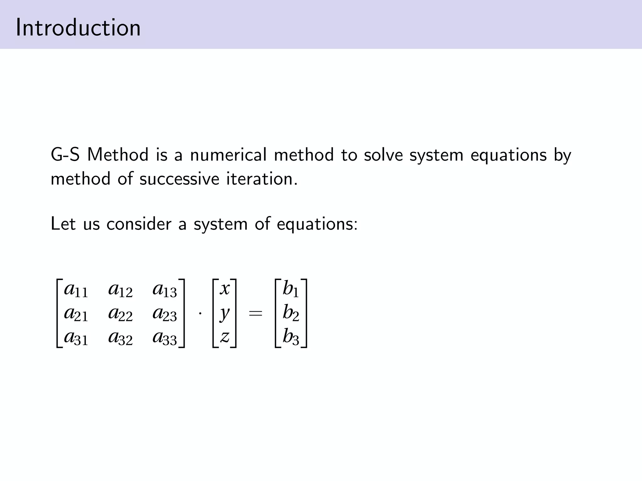
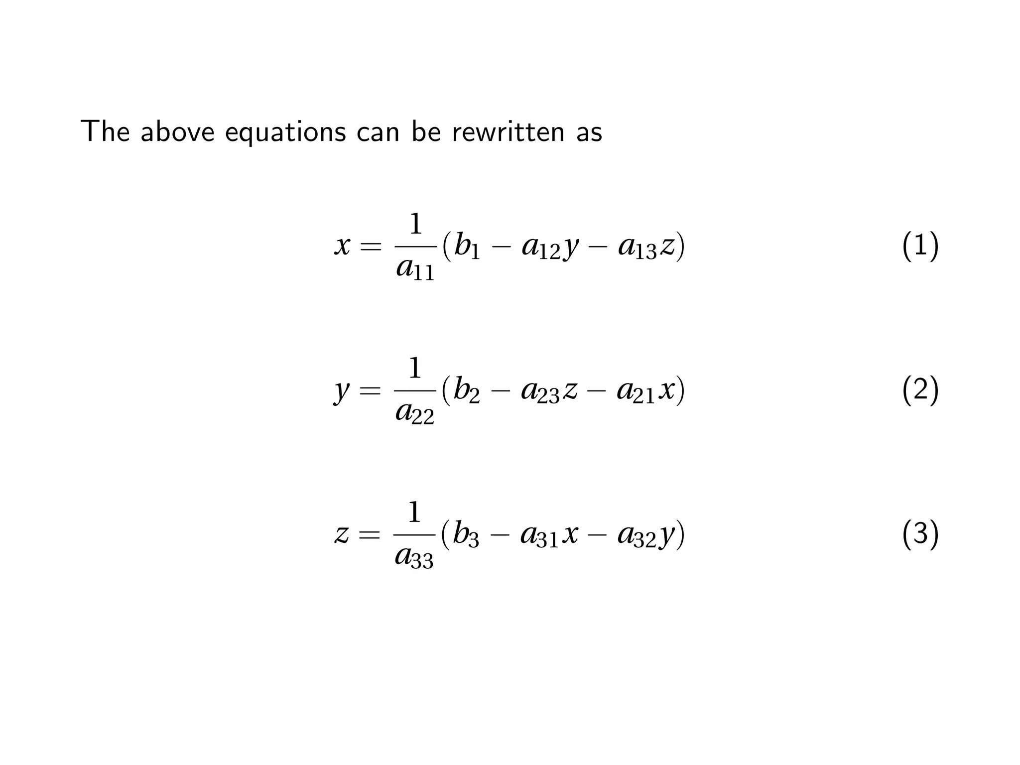
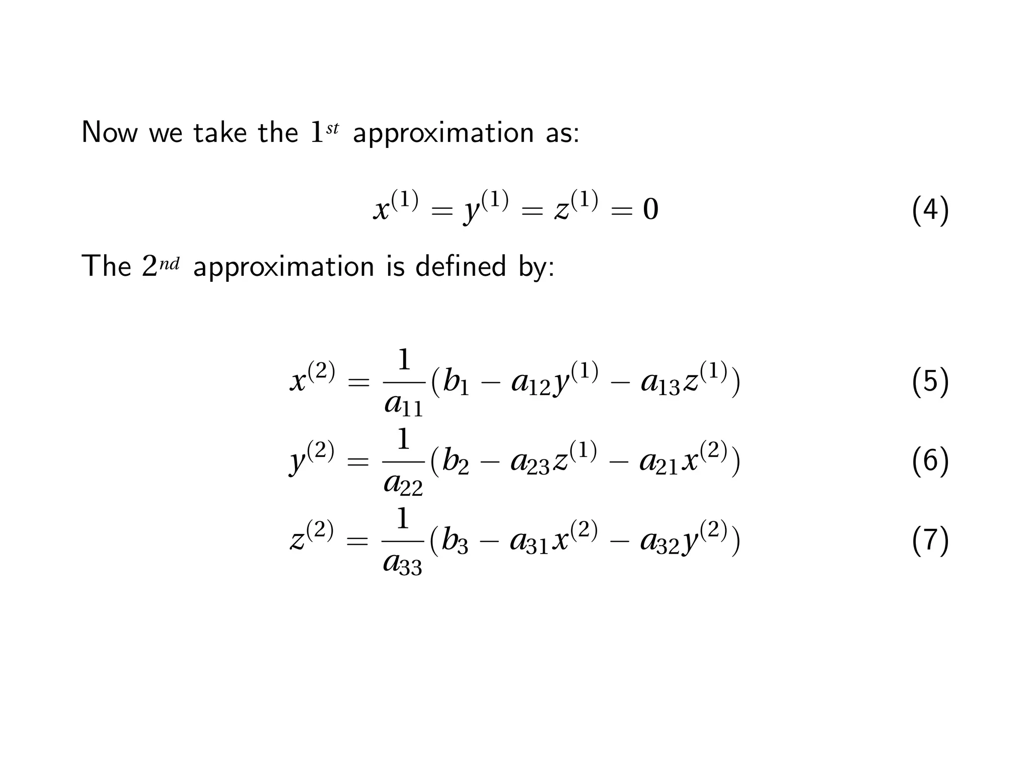
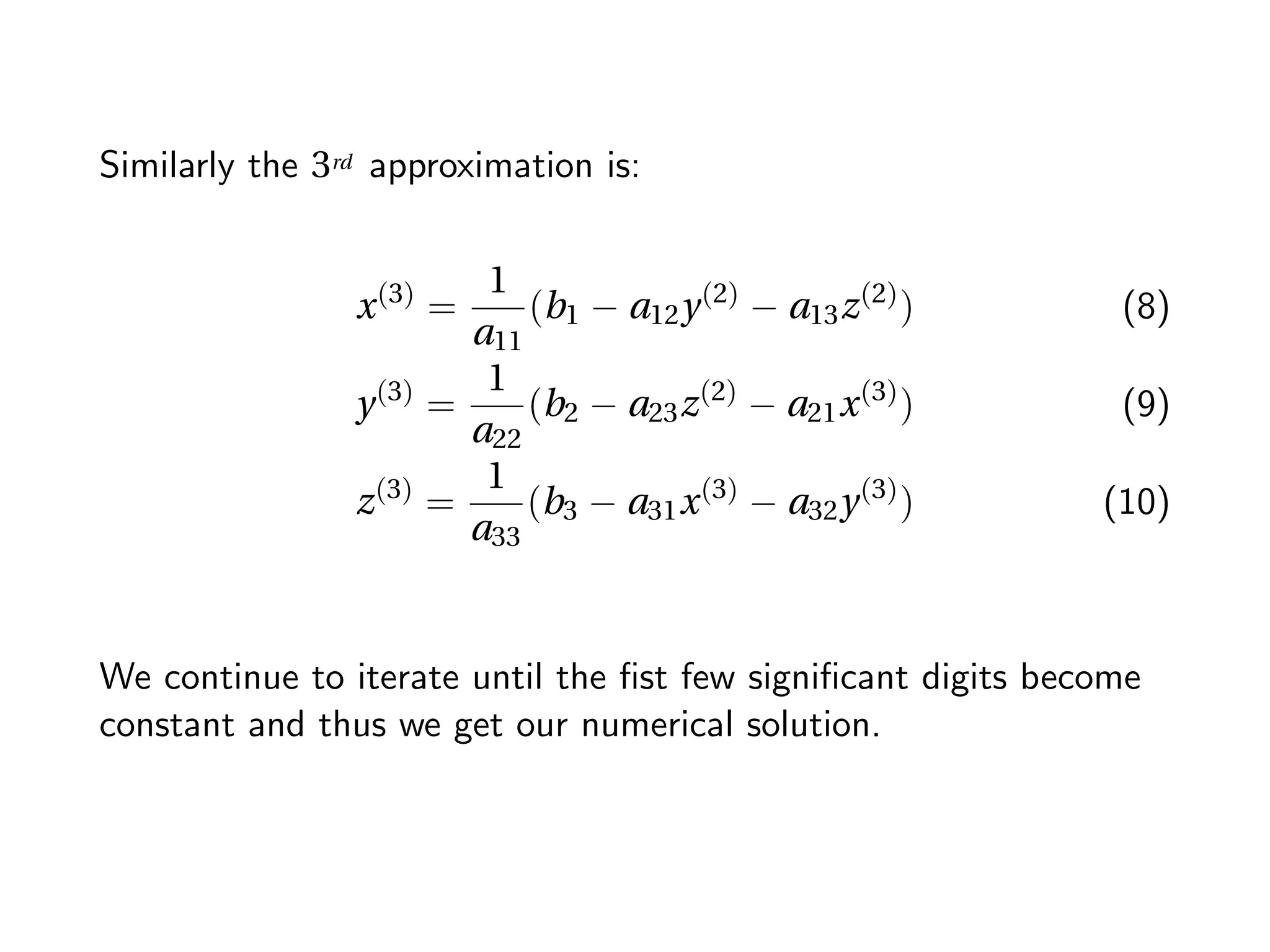
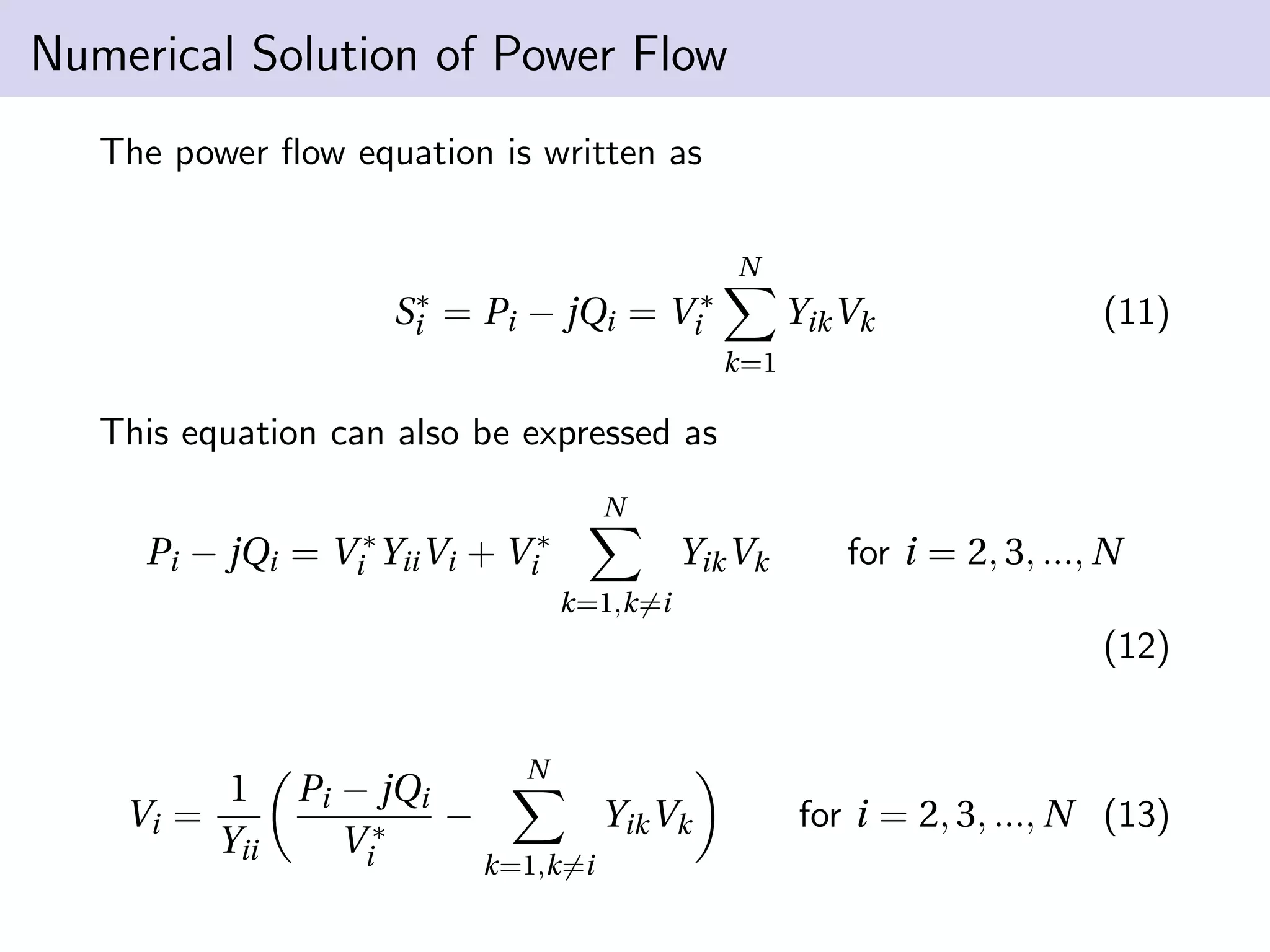
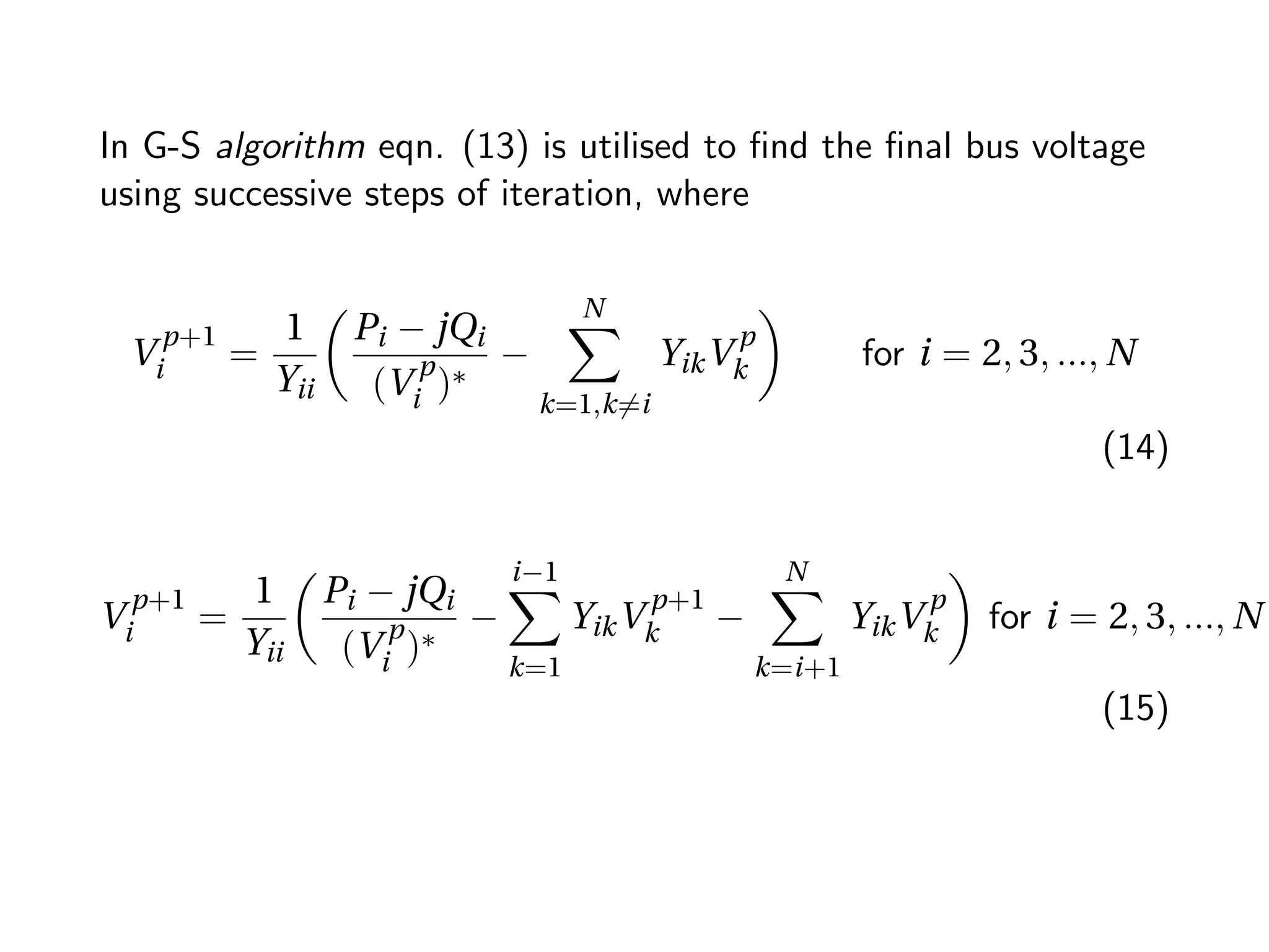
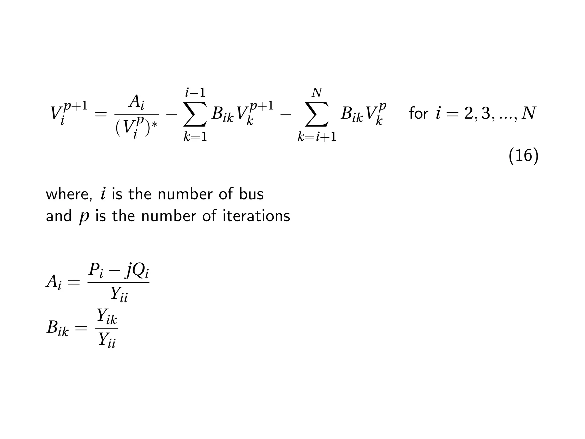
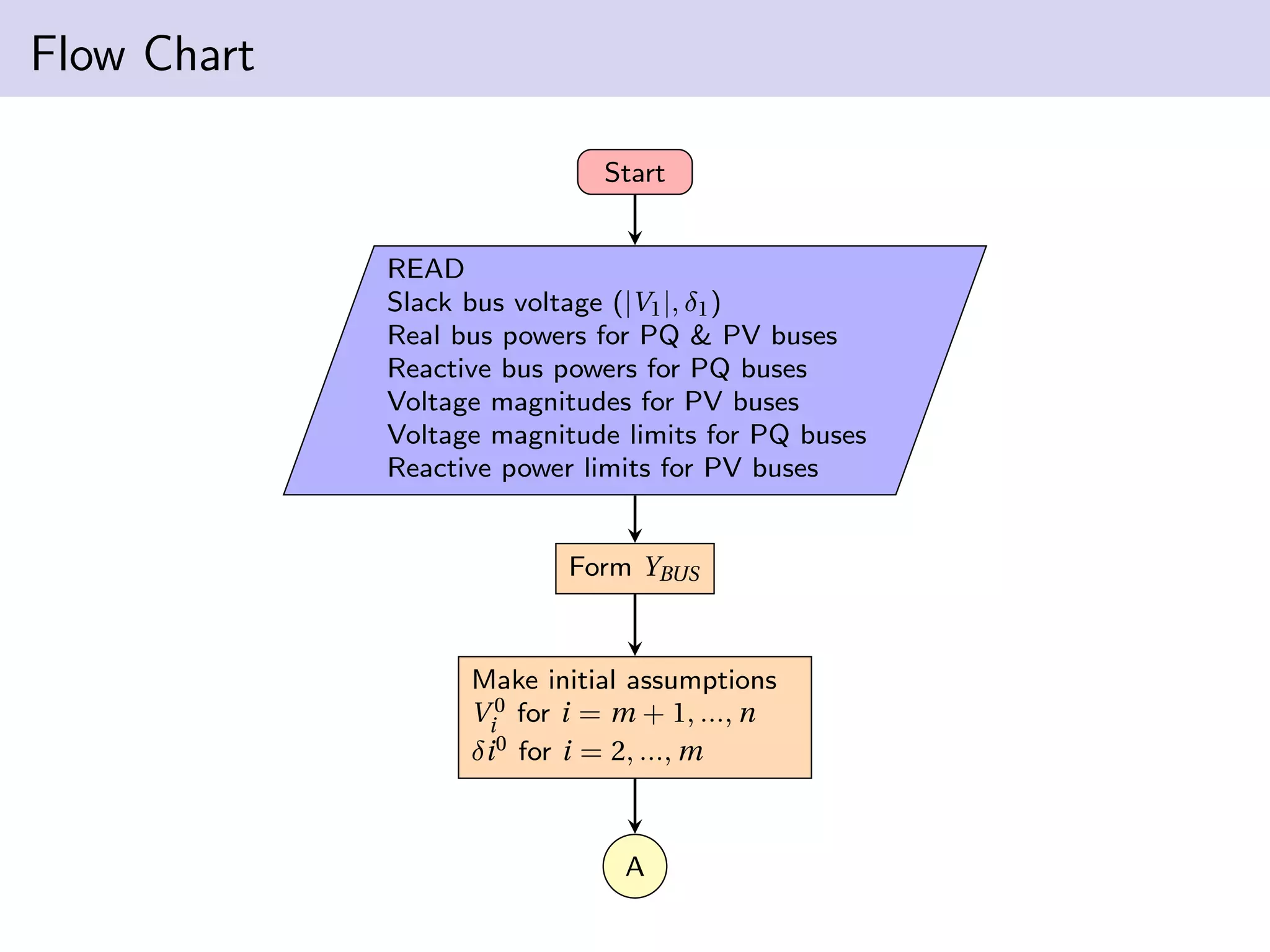
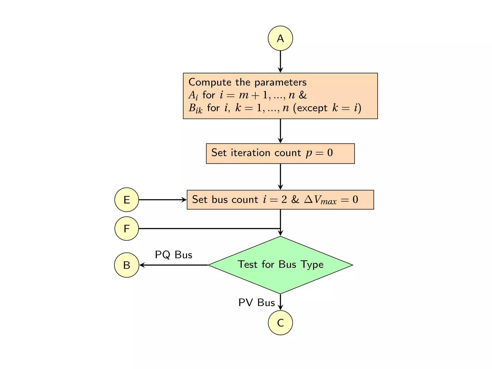
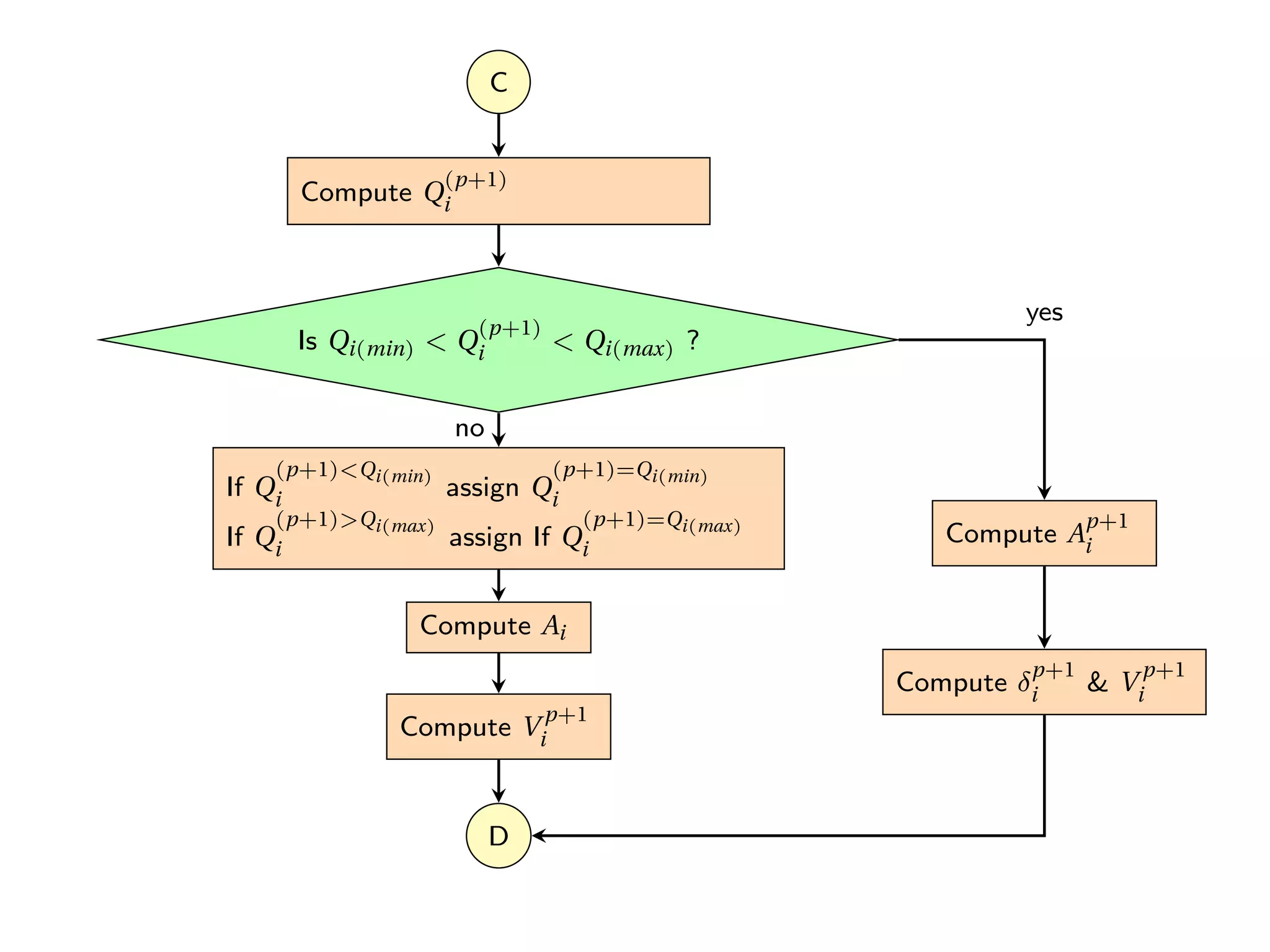
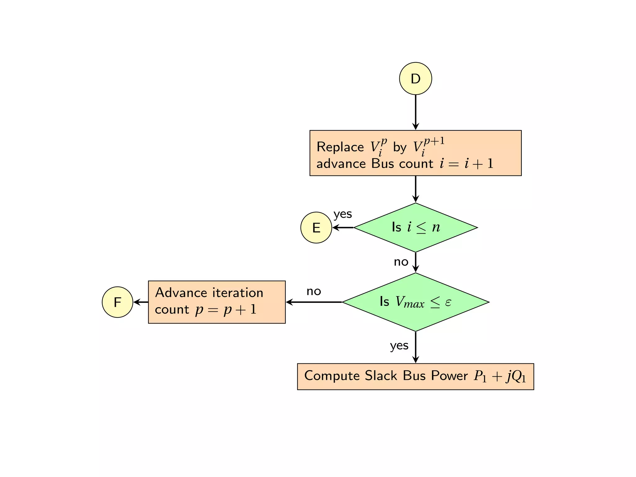
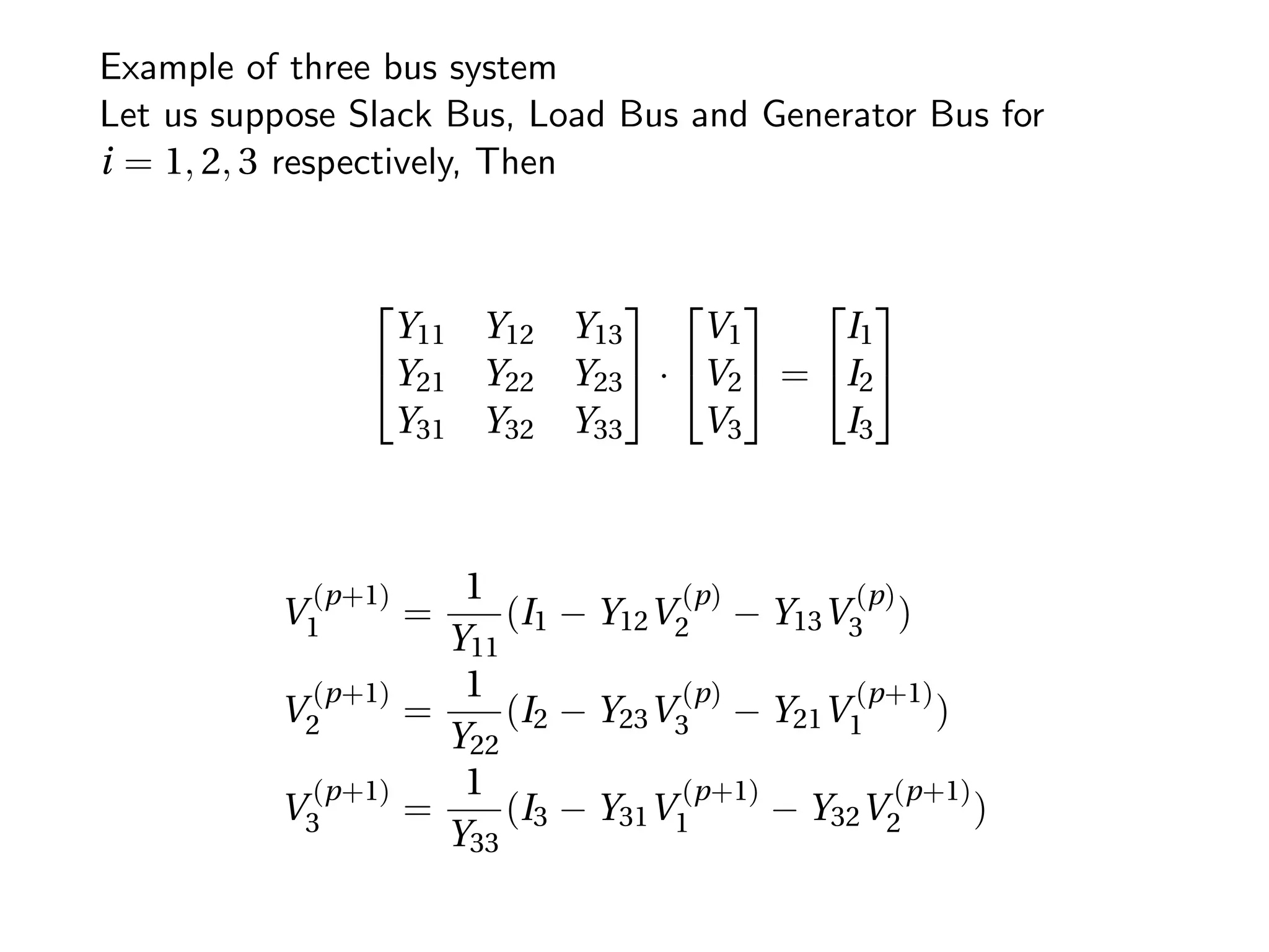
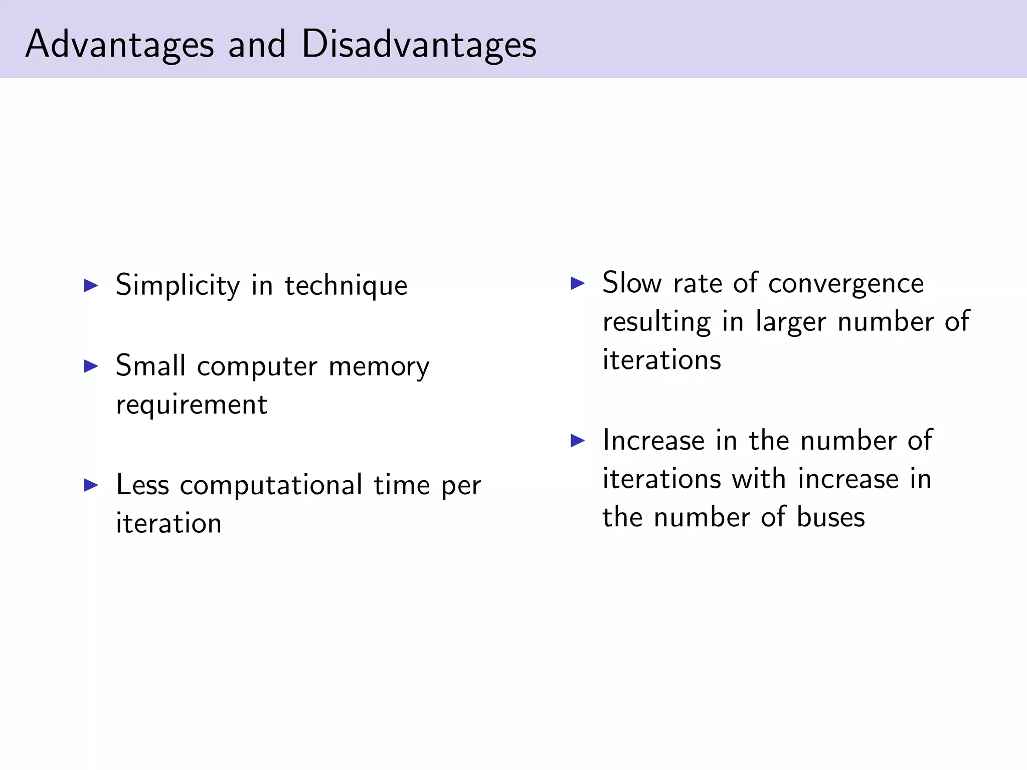
2. Table of Contents
Gauss Seidal Method
Application of G-S Method in Power Flow
Example
Advantages and Disadvantages

3. Table of Contents
Gauss Seidal Method
Application of G-S Method in Power Flow
Example
Advantages and Disadvantages

4. Introduction
G-S Method is a numerical method to solve system equations by
method of successive iteration.
Let us consider a system of equations:


a11 a12 a13
a21 a22 a23
a31 a32 a33

 ·


x
y
z

 =


b1
b2
b3



5. The above equations can be rewritten as
x =
1
a11
(b1 − a12y − a13z) (1)
y =
1
a22
(b2 − a23z − a21x) (2)
z =
1
a33
(b3 − a31x − a32y) (3)

6. Now we take the 1st approximation as:
x(1)
= y(1)
= z(1)
= 0 (4)
The 2nd approximation is defined by:
x(2)
=
1
a11
(b1 − a12y(1)
− a13z(1)
) (5)
y(2)
=
1
a22
(b2 − a23z(1)
− a21x(2)
) (6)
z(2)
=
1
a33
(b3 − a31x(2)
− a32y(2)
) (7)

7. Similarly the 3rd approximation is:
x(3)
=
1
a11
(b1 − a12y(2)
− a13z(2)
) (8)
y(3)
=
1
a22
(b2 − a23z(2)
− a21x(3)
) (9)
z(3)
=
1
a33
(b3 − a31x(3)
− a32y(3)
) (10)
We continue to iterate until the fist few significant digits become
constant and thus we get our numerical solution.

8. Table of Contents
Gauss Seidal Method
Application of G-S Method in Power Flow
Example
Advantages and Disadvantages

9. Numerical Solution of Power Flow
The power flow equation is written as
S∗
i = Pi − jQi = V ∗
i
N
k=1
YikVk (11)
This equation can also be expressed as
Pi − jQi = V ∗
i YiiVi + V ∗
i
N
k=1,k=i
YikVk for i = 2, 3, ..., N
(12)
Vi =
1
Yii
Pi − jQi
V ∗
i
−
N
k=1,k=i
YikVk for i = 2, 3, ..., N (13)

10. In G-S algorithm eqn. (13) is utilised to find the final bus voltage
using successive steps of iteration, where
V
p+1
i =
1
Yii
Pi − jQi
(V
p
i )∗
−
N
k=1,k=i
YikV
p
k for i = 2, 3, ..., N
(14)
V
p+1
i =
1
Yii
Pi − jQi
(V
p
i )∗
−
i−1
k=1
YikV
p+1
k −
N
k=i+1
YikV
p
k for i = 2, 3, ..., N
(15)

11. V
p+1
i =
Ai
(V
p
i )∗
−
i−1
k=1
BikV
p+1
k −
N
k=i+1
BikV
p
k for i = 2, 3, ..., N
(16)
where, i is the number of bus
and p is the number of iterations
Ai =
Pi − jQi
Yii
Bik =
Yik
Yii

12. Flow Chart
Start
READ
Slack bus voltage (|V1|, δ1)
Real bus powers for PQ & PV buses
Reactive bus powers for PQ buses
Voltage magnitudes for PV buses
Voltage magnitude limits for PQ buses
Reactive power limits for PV buses
Form YBUS
Make initial assumptions
V 0
i for i = m + 1, ..., n
δi0 for i = 2, ..., m
A

13. A
Compute the parameters
Ai for i = m + 1, ..., n &
Bik for i, k = 1, ..., n (except k = i)
Set iteration count p = 0
Set bus count i = 2 & ∆Vmax = 0
Test for Bus TypeB
C
E
F
PQ Bus
PV Bus

14. C
Compute Q
(p+1)
i
Is Qi(min) < Q
(p+1)
i < Qi(max) ?
If Q
(p+1)<Qi(min)
i assign Q
(p+1)=Qi(min)
i
If Q
(p+1)>Qi(max)
i assign If Q
(p+1)=Qi(max)
i
Compute A
p+1
i
Compute Ai
Compute V
p+1
i
Compute δ
p+1
i & V
p+1
i
D
no
yes

15. D
Replace V
p
i by V
p+1
i
advance Bus count i = i + 1
Is i ≤ n
Is Vmax ≤ ε
Advance iteration
count p = p + 1
Compute Slack Bus Power P1 + jQ1
E
F
yes
no
yes
no

16. Table of Contents
Gauss Seidal Method
Application of G-S Method in Power Flow
Example
Advantages and Disadvantages

17. Example of three bus system
Let us suppose Slack Bus, Load Bus and Generator Bus for
i = 1, 2, 3 respectively, Then


Y11 Y12 Y13
Y21 Y22 Y23
Y31 Y32 Y33

 ·


V1
V2
V3

 =


I1
I2
I3


V
(p+1)
1 =
1
Y11
(I1 − Y12V
(p)
2 − Y13V
(p)
3 )
V
(p+1)
2 =
1
Y22
(I2 − Y23V
(p)
3 − Y21V
(p+1)
1 )
V
(p+1)
3 =
1
Y33
(I3 − Y31V
(p+1)
1 − Y32V
(p+1)
2 )

18. V1 = 1 + j0
V
(p+1)
2 = 1
Y22
P2−jQ2
(V
p
2 )∗ − Y23V
(p)
3 − Y21V
(p+1)
1
Q
(p+1)
3 = − N
k=1 YikViVk = −(Y31V3V1 +Y32V3V
p+1
2 +Y33V3V3)
V
(p+1)
3 = 1
Y33
P3−jQ3
(V
p
3 )∗ − Y31V
(p+1)
1 − Y32V
(p+1)
2

19. Table of Contents
Gauss Seidal Method
Application of G-S Method in Power Flow
Example
Advantages and Disadvantages

20. Advantages and Disadvantages
Simplicity in technique
Small computer memory
requirement
Less computational time per
iteration
Slow rate of convergence
resulting in larger number of
iterations
Increase in the number of
iterations with increase in
the number of buses

21. Thank You