1) The document reviews and compares various implementations of the Discrete Cosine Transform (DCT), which is widely used in video and image compression standards. 2) It finds that the Loeffler algorithm achieves the theoretical minimum of 11 multiplications for an 8-point DCT, while the Arai algorithm requires only 5 multiplications and 29 additions. 3) The document concludes that while the DCT has been very successful, other transforms like the Discrete Wavelet Transform used in the Daala standard may provide alternatives worth further research to reduce blocking artifacts at high compression.

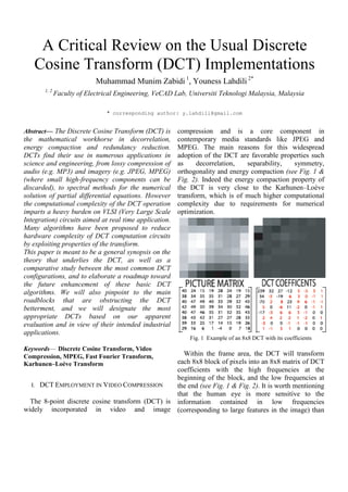
1. A Critical Review on the Usual Discrete
Cosine Transform (DCT) Implementations
Muhammad Munim Zabidi 1
, Youness Lahdili 2*
1, 2
Faculty of Electrical Engineering, VeCAD Lab, Universiti Teknologi Malaysia, Malaysia
* corresponding author: y.lahdili@gmail.com
Abstract— The Discrete Cosine Transform (DCT) is
the mathematical workhorse in decorrelation,
energy compaction and redundancy reduction.
DCTs find their use in numerous applications in
science and engineering, from lossy compression of
audio (e.g. MP3) and imagery (e.g. JPEG, MPEG)
(where small high-frequency components can be
discarded), to spectral methods for the numerical
solution of partial differential equations. However
the computational complexity of the DCT operation
imparts a heavy burden on VLSI (Very Large Scale
Integration) circuits aimed at real time application.
Many algorithms have been proposed to reduce
hardware complexity of DCT computation circuits
by exploiting properties of the transform.
This paper is meant to be a general synopsis on the
theory that underlies the DCT, as well as a
comparative study between the most common DCT
configurations, and to elaborate a roadmap toward
the future enhancement of these basic DCT
algorithms. We will also pinpoint to the main
roadblocks that are obstructing the DCT
betterment, and we will designate the most
appropriate DCTs based on our apparent
evaluation and in view of their intended industrial
applications.
Keywords— Discrete Cosine Transform, Video
Compression, MPEG, Fast Fourier Transform,
Karhunen–Loève Transform
I. DCT EMPLOYMENT IN VIDEO COMPRESSION
The 8-point discrete cosine transform (DCT) is
widely incorporated in video and image
compression and is a core component in
contemporary media standards like JPEG and
MPEG. The main reasons for this widespread
adoption of the DCT are favorable properties such
as decorrelation, separability, symmetry,
orthogonality and energy compaction (see Fig. 1 &
Fig. 2). Indeed the energy compaction property of
the DCT is very close to the Karhunen–Loève
transform, which is of much higher computational
complexity due to requirements for numerical
optimization.
Fig. 1 Example of an 8x8 DCT with its coefficients
Within the frame area, the DCT will transform
each 8x8 block of pixels into an 8x8 matrix of DCT
coefficients with the high frequencies at the
beginning of the block, and the low frequencies at
the end (see Fig. 1 & Fig. 2). It is worth mentioning
that the human eye is more sensitive to the
information contained in low frequencies
(corresponding to large features in the image) than

2. Equation 1
to the information contained in high frequencies
(corresponding to small features). Therefore, the
DCT helps separate the more perceptually
significant information from less perceptually
significant information.
The DCT itself is not lossy; that is, an inverse
DCT (IDCT) could be used to perfectly reconstruct
the original. The DCT is a reversible and lossless
operation, meaning that the encoder and the
decoder do the exact same thing, and that it does
not directly help data compression, but just
reorganize the coefficients of a block by frequency
order, so that later on we can nullify the highest
frequencies coefficients by using an arbitrarily
quantization mask.
Fig. 2 Theoretical representation of an 8x8 DCT
II. THEORY ON DISCRETE COSINE TRANSFORM
A discrete cosine transform (DCT) expresses a
finite sequence of data points in terms of a sum of
cosine functions oscillating at different frequencies.
The use of cosine rather than sine functions is
critical in these applications. For compression, it
turns out that cosine functions are much more
efficient (fewer functions are needed to
approximate a typical signal) (see Fig. 3), whereas
for differential equations the cosines express a
particular choice of boundary conditions.
Fig. 3 DCT can approximate a line with less coefficients than
FFT would do
In particular, a DCT is a Fourier-related
transform similar to the discrete Fourier transform
(DFT), but using only real numbers. DCTs are
equivalent to DFTs of roughly twice the length,
operating on real data with even symmetry (since
the Fourier transform of a real and even function is
real and even). There are eight standard DCT
variants, of which four are common.
The most common variant of discrete cosine
transform is the type-II DCT, which is often called
simply "the DCT", its inverse, the type-III DCT, is
correspondingly often called simply "the inverse
DCT" or "the IDCT". Two related transforms are
the discrete sine transform (DST), which is
equivalent to a DFT of real and odd functions, and
the modified discrete cosine transform (MDCT),
based on the DCT-IV and used in AAC, Vorbis,
WMA, and MP3 audio compression.
III. CALCULATION OF DISCRETE COSINE TRANSFORM
A. Algebraic Principle of DCT
The DCT that is widely used in regard with data
compression was introduced by N. Ahmed, T.
Natarajan and K. R. Rao in 1974. The DCT
transform for N-point is given by the following
trigonometric formula:
With:

3. The DCT, and in particular the DCT-II, is often
used in signal and image processing, especially for
lossy data compression, because it has a strong
"energy compaction" property: most of the signal
information tends to be concentrated in a few low-
frequency components of the DCT, approaching the
Karhunen-Loève transform (KLT). KLT is the
optimal transform in the decorrelation of a signal,
yet there was no efficient algorithm available to
compute the KLT. DCT evolved as the most viable
approximation of KLT.
Multidimensional variants of the various DCT
types follow straightforwardly the one-dimensional
definitions: they are simply a separable product
(equivalently, a composition) of DCTs along each
dimension. For example, a two-dimensional DCT-II
of an image or a matrix is simply the one-
dimensional DCT-II, from above, performed along
the rows and then along the columns (or vice versa).
This technique is exposed in the following segment.
B. Technique to obtain 2D DCT out of 1D DCT
The two-dimensional (2D) discrete cosine
transform (DCT) of an NxN matrix could be easily
built by applying 1D DCT to each of the columns
for N times then we re-apply again the same
process, but this time after we transpose the
resulting matrix from first process (see Fig. 4).
Fig. 4 Practical 2D DCT computing
The 2D DCT is a fundamental operation in real-
time video systems, which is adopted in
compression standards, such as JPEG, VP9, MPEG
family with their most recently H.265/HEVC. The
DCT is the de-facto standard in transform coding
due -as we mentioned earlier- to its superior energy
aggregation on par with the optimum Karhunen–
Loève transforms, achieved at reasonably low
computational complexity.
The circuit realization of the 2D 8x8 DCT affects
noise, distortion, circuit area, and power
consumption of such compression systems. The 2D
DCT implementation is essentially dependent on
the 1D DCT. The 8-point 1D DCT requires
multiplications by numbers in the form cos(nπ/16).
These constants impose implementation difficulties
in terms of their machine representation, because
they are irrational values. Fixed-point arithmetic
DCT implementations usually employ rounding off
to approximate such quantities, which introduces
errors. Besides the numerical representation issues,
error propagation, noise injection, noise coupling,
and noise amplification are significant when
considering fixed-point realizations.
In the remaining of this paper, we will present
some of the key DCT algorithms that were devised
and published since DCT was first discovered, and
are still used until today. Similarly to FFT, these
algorithms compute DCT faster than by using the
trigonometric transform directly, and that is why
they carry the name of Fast DCTs. They will be
essentially gauged for use in the course of this
review paper.
C. Measuring the differences between the DCTs
Algorithms
Different algorithms to compute the 1D DCT
have been proposed in recent years, all of the most
need 12 multiplications and 29 additions to
complete an 8-point DCT:
Author/Ref. Multiplications Additions
Chen 16 (13) 26 (29)
Wang 13 29
Lee 12 29
Vetterli 12 29
Suehiro 12 29
Hou 12 29
Loeffler 11 29
Tab. 1 Summary of DCT schemes and their arithmetic
operations counts
1) Chen's Fast DCT algorithm, the first one
published, exhibits a very regular structure. The
published number of multiplications and additions

4. where:
Equation 2
can easily be changed to the numbers shown in parenthesis in table above by using the same method to
calculate a rotation as is used in all later publications (3 multiplications and 3 additions per rotation).
Chen’s ground work was to factorize the original DCT trigonometric formula and rewrite it into the
following matrix (Look-up Table) decomposition:
This algorithm is by far the most popular and widely treated. It is easier to grasp its flow by representing
its routine as a butterfly diagram, which also offer a better view on which operation are to be carried out in
parallel.
Fig. 5 Butterfly Flowgraph of Chen’s Method to Calculate 8-point 1D DCT
2) Wang has a method to easily obtain algorithms
for the Discrete Sine Transform (DST), the Discrete
W-Transform (DWT) and the Discrete Fourier
Transform (DFT) from his DCT algorithm.
3) Lee's algorithm has very regular first stages,
but has irregular data flow in the last stage and
needs the inverse of cosine values as coefficients.
This can lead to numerical overflow problems.
4) Vetterli uses a recursive formula for his
algorithm; however, additional operations required
to connect the recursively calculated blocks lead to
an increased complexity in the communication
structure of his algorithm.
5) Suehiro needs fewer multiplications than
Wang, but his solution still allows applying Wang's

5. method to obtain algorithms for DST, DWT and
DFT from the DCT algorithm.
6) Hou proposes a recursive algorithm, basing
each DCT of length N on two DCTs of length N/2.
The algorithm is regular, with the exception of the
last stage, where some irregularities are introduced
for larger lengths.
7) Duhamel shows that the theoretical lower
bound for an 8-point DCT is 11 multiplications.
This result is obtained by looking at the DCT as an
algorithm based on a cyclic convolution, and
applying methods of Winograd. Heidemann came
to the same result.
8) It follows that most of the published
algorithms for an 8-point Discrete Cosine
Transform use only one multiplication more than
the theoretical minimal number required. Except for
one algorithm, the Loeffler algorithm, which
successfully brought the number of multiplication
required to 11 (indeed the lower bound possible),
without an increase in the number of additions.
Here is its representation:
Fig. 6 Butterfly Flowgraph of Loeffler’s Method to Calculate 8-point 1D DCT
9) However, there are some special solutions,
which require fewer multiplications for the actual
DCT, but move the complexity to another part of
the calculation. Examples for these include a
solution based on number theoretical transforms
requiring only 8 multiplications for an 8 bit DCT
explained in Duhamel's paper and the Arithmetic
Fourier Transform. The first example causes
additional costs for signal transformation and
increased word-length, the second one requires
unequally spaced sampling instants for the signal.
Therefore both examples do not lead to overall
less complex solutions than the algorithms
mentioned before.
10) We have also knew of the existence of 2D
DCT algorithms that require less arithmetic moves
than when two 1D DCTs are used in tandem as
usually done. We are making allusion to Feig
algorithm, and Arai algorithm. This latter for which
the referential 1D DCT version is shown in Fig. 7
as a butterfly diagram.

6. Fig. 7 Butterfly Flowgraph 8-point DCT adapted from Arai
a1 = 0,707; a2 = 0,541; a3 = 0,707; a4 = 1,307; and a5 = 0,383
The small arrow means negation and black bubble is addition
All these aforementioned special 2D DCTs are
benefiting from the fact that the repetition of 1D
DCT for twice can be traded-off.
11) Graphical-based method to compute 2D DCT
directly
Another intuitive method to calculate DCT for an
8x8 block of pixels, is to specially multiply the
image block with the predefined DCT 8x8 basic
pattern which is normally arranged by frequency
order, where each step from left to right and top to
bottom is an increase in frequency by ½ cycle.
Using a mathematical computing environment
like MATLAB® will make this method faster than
the previously mentioned ones and less
cumbersome in term of coding. This sophisticated
numerical development software is inherently built
to perform the special multiplication than will yield
to this 2D DCT method. For this end, one can
simply generate the constant-valued DCT 8x8 basic
pattern by using the internal MATLAB® function
dctmtx(8), before he can actually perform the
8x8 matrix twice dotted multiplication.
Fig. 8 besides will illustrates the basic concept
behind this method and an insinuation on how to
perform this 2D DCT computation graphically:
Fig. 8 Decomposition of Predefined DCT 8x8 Basic Pattern
IV.CONCLUSION
So as a recapitulation of our comparative review
on prior DCT schemes, we affirm that there are a
multitude of fast algorithms used for the
computation of the DCT. The direct-form
realization in Chen scheme provides a
straightforward method for DCT computation but
results in increased chip area. However, this scheme
has a regular and modular structure which is of
advantage in stability in digital circuits.
Algorithms that use recursive calculations to
compute the N-point DCT from two N/2-point
DCTs have been proposed by Lee and Hou using a
scheme similar to the Cooley–Tukey FFT algorithm.
Vetterli proposed an algorithm which computes
an N-point DCT from an N/4-point DCT and an
N/2-point DFT, thus involving three degrees of
recursion. These recursive DCT algorithms require
(N/2)log2 N real multiplications.
Duhamel showed that the theoretical lower bound
for an 8-point DCT is 11 multiplications and a class
of DCT algorithms achieving this lower bound is
presented in by Loeffler.
Arai however proposed a scheme where this
computation can be efficiently achieved in cases
where the explicit values of DCT coefficients are
not required.

7. Digital video compression start getting adapted to
the Arai algorithm, which in turn is based on the
findings of Tseng who showed that the 8-point
DCT can be computed by the means of the real part
of 16-point DFT. Only five multiplications and
twenty-nine additions are needed for this method,
hence superseding the other algorithms mentioned
in terms of multiplier complexity.
If the explicit values of the 8-point DCT are
required, the output values computed from the Arai
algorithm have to be multiplied by scalar constants.
Fortunately, this step can be absorbed by the
quantizer in the video compression engine without
increasing the arithmetic complexity.
The signal flow graph of the Arai algorithm has
been previously reviewed in Fig. 8, but there
coexist other variants of this butterfly diagram.
V. ADVERSE ISSUES PERTAINING TO DCT
DEPLOYMENT
At higher level of compression, the DCT
introduces some blocking artifacts, so other
methods, such as fractal compression, matching
pursuit and the use of a discrete wavelet transform
(DWT) have been the subject of some research, but
are typically not used in practical products (except
for the use of wavelet coding as still-image coders
without motion compensation). DWT a powerful
tool for compressing information, represents
pictures, as waves that can be described
mathematically in terms of frequency, energy and
time. The Daala standard however is using DWT
instead of DCT. Interest in fractal compression
seems to be waning, due to recent theoretical
analysis showing a comparative lack of
effectiveness of such methods.
In relation with complexity, a recurrent obstacle
in performing accurate DCT computations is the
implementation of the irrational coefficients in the
transform.
Another problem with DCT is that computing it
takes a large (sometime the largest) share on the
overall video compression processing time. There
are many researches that aimed at finding a suitable
architecture for DCT that will ensure rapidity of
calculation and precision of the output DCT
coefficients. But there were always caveats that
needed to be tackled, and not every proposed DCT
algorithm is suited for every application targeted.
So there is a pressing need to find the best
solution to calculate DCT coefficients with
minimum computation time, less arithmetic moves
and closest coefficients to the real DCT found
algebraically. Attempts to make up for this need are
under study.
VI.REFERENCES
[1] N. Ahmed, T. Natarajan, and K. R. Rao (1974).
"Discrete Cosine Transform" IEEE Trans. Computer, vol.
COM-23, no. 1, pp. 90-93.
[2] Nasir Ahmed (1991) "How I Came Up with the Discrete
Cosine Transform" Digital Signal Processing 1, 4-5.
[3] W. A. Chen , C. Harrison and S. C. Fralick (1977). "A
Fast computational Algorithm for the Discrete Cosine
Transform", IEEE Transactions on
Communications, vol. COM-25, no. 9, pp.1004-1011.
[4] S. Winograd (1977) "Some bilinear Forms whose
multiplicative Complexity depends on the Field of
Constants", Math. System Theory, vol. 10, pp.169-180.
[5] B. Tseng. and W. Miller (1978). "On computing the
discrete cosine transform" IEEE Trans. Comput. C-27,
pp. 966-968.
[6] A. K. Jain (1979). "A sinusoidal family of unitary
transform" IEEE Trans. Pattern Anal. Mach. Intell., vol.
PAMI-I, pp. 356-365.
[7] Z. Wang and B. R. Hunt (1983). "The discrete cosine
transform-A new Version", in Proc. Int. Conf. Acoust.,
Speech, Signal Processing.
[8] Z. Wang (1984). "Fast algorithms for the discrete W
transform and for the discrete Fourier transform" IEEE
Trans. Acoust., Speech, Signal Process. vol. ASSP-32,
no.4, pp. 803-816.
[9] B. Lee (1984). "A new algorithm to compute the discrete
cosine transform" IEEE Trans. Acoust. Speech Signal
Process, 32, pp. 1243-1245.
[10] M. Vetterli and H. Nussbaumer (1984). "Simple FFT and
DCT Algorithms with Reduced Number of

8. Operations", Signal Processing (North Holland), vol.
6, no. 4, pp.267-278
[11] M. Vetterli and A. Ligtenberg (1986). "A Discrete
Fourier-Cosine Transform Chip", IEEE Journal on
Selected Areas of Communications, vol. SAC-4, no.
1, pp.49-61
[12] N. Suehiro and M. Hatori (1986). "Fast Algorithms for
the DFT and other Sinusoidal Transforms", IEEE
Transactions on Acoustics, Speech, and Signal
Processing, vol. ASSP-34, no. 3, pp.642-644.
[13] H. Hou (1987). "A fast recursive algorithm for
computing the discrete cosine transform" IEEE Trans.
Acoust. Speech Signal Process, 35, pp. 1455-1461.
[14] P. Duhamel and H. H’Mida (1987). "New 2n
DCT
Algorithms Suitable for VLSI Implementation". In
Proceedings of the IEEE International Conference on
Acoustics, Speech, and Signal Processing (ICASSP ’87),
Boston, MA, USA, Volume 12, pp. 1805-1808.
[15] Y. Arai, T. Agui and M. Nakajima (1988). "A fast DCT-
SQ scheme for images". Trans. IEICE , e 71, pp. 1095-
1097.
[16] C. Loeffler, A. Ligtenberg and G. Moschytz (1989).
"Practical Fast 1-D DCT Algorithms with 11
Multiplications". In Proceedings of the IEEE
International Conference on Acoustics, Speech, and
Signal Processing (ICASSP ’89), Glasgow, Scotland,
Volume 2, pp. 988-991.
[17] N.I Cho and S. U. Lee (1991). "Fast Algorithm and
Implementation of 2-D Discrete Cosine
Transform", IEEE TRANS. CIRCUIT AND
SYSTEM, vol. 38, no. 3
[18] W.H. Chen , C.H. Smith and S.C. Fralick (1991). "A Fast
Computational Algorithm for the Discrete Cosine
Transform", IEEE Trans. Circuit and System, vol. Com.
25, no. 9, pp.1004 -1009.
[19] G. Zhang and A. Pan (1992). "The Theory and
Applications of Digital Spectrum Method" Beijing:
Defence Industry Press.
[20] W.B. Pennebaker and J.L. Mitchell (1993). "JPEG Still
Image Data Compression Standard. Van Nostrand
Reinhold".
[21] J. Blinn (1993). "What’s that deal with the DCT" IEEE
Comput. Graph. Appl., 13, pp. 78-83.
[22] S. A. Martucci (1994). "Symmetric Convolution and the
Discrete Sine and Cosine Transforms," IEEE Trans. on
Signal Processing, vol. 42, pp. 1038-1051.
[23] V. Dimitrov, G. Jullien and W, Miller (1998). "A New
DCT Algorithm Based on Encoding Algebraic Integers"
In Proceedings of the IEEE International Conference on
Acoustics, Speech and Signal Processing, Seattle, WA,
USA, Volume 3, pp. 1377-1380.
[24] Z. Mohd-Yusof, I. Suleiman, and Z. Aspar (2000)
"Implementation of two dimensional forward DCT and
inverse DCT using FPGA," in TENCON 2000.
Proceedings, vol. 3, pp. 242-245 vol.3.
[25] V. Dimitrov, K. Wahid and G. Jullien (2004).
"Multiplication-free 8 × 8 2D DCT architecture using
algebraic integer encoding" Electron. Lett., 40, pp.
1310-1311.
[26] D. Gong, Y. He and Z. Cao (2004). "New cost-effective
VLSI implementation of a 2-D discrete cosine transform
and its inverse". IEEE Trans. Circuits Syst. Video
Technol., 14, pp. 405-415.
[27] N.J. August and Dong Sam Ha (2004). "Low power
design of DCT and IDCT for low bit rate video codecs"
IEEE Trans. Multimedia, Vol. 6, no.3, pp. 414- 422.
[28] S. Ghosh, S. Venigalla and M. Bayoumi (2005). "Design
and Implementaion of a 2D-DCT Architecture Using
Coefficient Distributed" In Proceedings of the IEEE
Computer Society Annual Symposium on VLSI, Tampa,
FL, USA, pp. 162-166.
[29] V. Britanak, P. Yip and K.R. Rao (2007). "Discrete
Cosine and Sine Transforms" Academic Press: Waltham,
MA, USA.
[30] D. Kunz (2008). "An orientation-selective orthogonal
lapped transform" IEEE Trans. Image Process., vol. 17,
no. 8, pp.1313-1322.
[31] R.J. Cintra and F.M. Bayer (2011). "A DCT
approximation for image compression" IEEE Signal
Process. Lett., 18, pp. 579-583.
[32] A.V. Oppenheim and R.W. Schafer (1975). "Discrete-
Time Signal Processing", Prentice Hall.
[33] K. R. Rao, and P. Yip (1990). "Discrete Cosine
Transform: Algorithms, Advantages, Applications",
Academic Press.