These are the lecture notes for Machine Learning course offered by Stanford University on Coursera.

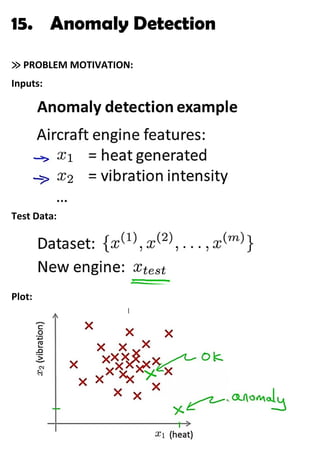
1. 15. Anomaly Detection
≫ PROBLEM MOTIVATION:
Inputs:
Test Data:
Plot:

2. Problem: we are given some training examples. We assume them
to be NON-ANOMALOUS. So, we need to find if a new example is
anomalous or not.
We train a PROBABILITY MODEL:
It divides the plot into various regions, such that each region
corresponds to a level of provability.
Centre → highest probability
Outside → lowest P

3. Example:
≫ GAUSSIAN DISTRIBUTION:

4. Examples:
σ → controls the width and height of curve
µ → mean of all values of x: controls the center..
Area below the curve is always = 1
So, the curve is either taller or wider.

5. Estimation of µ and σ :
≫ ALGORITHM FOR ANOMALY DETECTION:
Each feature can be individually distributred using
Normal(Gaussian) distribution:

6. P( x ) = product of probabilities of individual features
Note:
Steps of algorithm:

7. Example:
Gaussian Curves of both features:

8. P( x ) → height of curve == P(x1 ; µ1 , σ2
2) x P(x2 ; µ2 , σ2
2)
For a new example:

9. This means that anything below a particular height in the plot,
given by ϵ : is an anomaly
OR
Anything outside the learned region is an anomaly:
i.e., everything outside the magenta curve:
≫ DEVELOPING ANOMALY DETECTION SYSTEM:
Anomaly detection system problem can be converted to a likes of
Supervised Learning problem.
Therefore:

10. Thus we can take:
Meaning all the training set examples are non-anomalous
In Cross validation set and test set, we can have some examples of
anomalous (y=1) and some of non-anomalous (y=0) type:
Example:

11. ≫ How to evaluate the algorithm:
≫ How to choose ϵ :
We can choose the value of ϵ which gives the best value of F1 score.
Anomaly detection vs Supervised Learning:
In anomaly detection, it’s better to model anomalies based on
negative examples, rather than positive examples… as future
anomalies may be totally different.

12. Applications of Anomaly detection vs Supervised Learning:
Fraud detection can be a supervised learning application but only if
there are a lot of people on the website who are doing fraudulent
activity, i.e., most of the examples are positive, otherwise, it’s an
anomaly detection problem only
≫ Choosing what features to use:
We plot the data and the histogram looks like :
We’d be happy to see this as this means that the feature x is a
gaussian feature

13. But: if the histogram looks like:
This is a non gaussian distribution
So, we use different transforms on our data to make it as close as
possible to a gaussian distribution:
➔ These are feature v/s P( x )
We can use different transforms for different features to make
them gaussian features:
We may have to try out different transforms for the same feature
to find the best (which gives the best gaussian look to the data).

14. These parameters in the red are parameters we can vary to make
the data look more and more Gaussian.
≫ Coming up with features:
Error analysis method:

15. If there is an anomalous example in middle of some non-anomalous
examples, then the algo will fail.
➢So, we can look at that particular example and try to come up
with a new feature that can tell what went wrong with that
example
Example:

16. It may occur that if one of the computers is stuck in an infinite loop,
the CPU load grows but the network traffic doesn’t:
Then we can come up with a new feature:
OR
≫ MULTIVARIATE GAUSSIAN DISTRIBUTION:

17. Here, red points are training data
Green point is our test data
➢Lets look at both features individually:
The algo will not predict the right o/p … since the i/p data is
distributed on the whole axis, so all the points have some
probability of being correct.

18. Probability Contours:
To solve this:

19. Examples:
If we decr Σ :

20. If we incr Σ :
If we decr the variance of only one of the features:
OR

21. If we incr the variance of only one of the features:
OR

22. Other variations in Σ :

23. Varying the mean ( µ ): it moves the centre of contours, where
the probability ( P( x ) ) is highest.

24. ≫ Multivariate Gaussian Distribution Algorithm:
Algorithm:

25. ≫ Relationship of multivariate Gaussian Model with
Original Gaussian Model:
Original gaussian model is actually a special case of multivariate
model, in which, the contours have their axes aligned with the
features axes, i.e., the contours are not at nay angles:
Original model is mathematically the multivariate model with a
constraint, that is:

26. ≫ WHEN TO USE ORIGINAL MODEL vs MULTIVARIATE MODEL:
➢In some cases, in original model, we may require to manually
create extra features, so that the model can work fine.
➢In case of multivariate model, its important to get rid of
redundant features, o/w the algo is very expensive, and Σ may
even be non-invertible
…………………………………………………………………………………………………………
…………………………………………………………………………………………………………