Detailed Article on Anomaly Detection using Gaussian Models (Both Uni-Variate and Multi-Variate Gaussian Models)

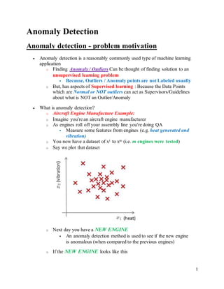
1. 1
Anomaly Detection
Anomaly detection - problem motivation
 Anomaly detection is a reasonably commonly used type of machine learning
application
o Finding Anomaly / Outliers Can be thought of finding solution to an
unsupervised learning problem
 Because, Outliers / Anomaly points are not Labeled usually
o But, has aspects of Supervised learning : Because the Data Points
which are Normal or NOT outliers can act as Supervisors/Guidelines
about what is NOT an Outlier/Anomaly
 What is anomaly detection?
o Aircraft Engine Manufacture Example:
o Imagine you're an aircraft engine manufacturer
o As engines roll off your assembly line you're doing QA
 Measure some features from engines (e.g. heat generated and
vibration)
o You now have a dataset of x1 to xm (i.e. m engines were tested)
o Say we plot that dataset
o Next day you have a NEW ENGINE
 An anomaly detection method is used to see if the new engine
is anomalous (when compared to the previous engines)
o If the NEW ENGINE looks like this

2. 2
 Probably OK - looks like the ones we've seen before
o But if the NEW ENGINE looks like this
o
 Uh oh! - this looks like an Anomalous Data-point
 More formally
o We have a Dataset which contains Normal (data)
 How we ensure they're normal is up to us
 In reality it's OK if there are a few which aren't actually normal
o Using that dataset as a reference point we can see if other examples
are Anomalous/Outliers
 How do we do this?

3. 3
o First, using our training dataset we build a model for Normal data points
 We can access this model using p(x)
 "What is the probability that Test example xtest is normal"
o Having built a model
 if p(xtest) < ε --> flag this as an Anomaly/Outlier
 if p(xtest) >= ε --> this is OK (Not Anomaly)
 ε is some threshold probability value which we define, depending
on how sure we need/want to be
o We expect our model to (graphically) look something like this;
 i.e. this would be our model if we had 2D data
Applications of Anomaly / Outlier Detection Algorithms
 Fraud detection in Login/Web resource Access/ Credit Card Usage etc.
o Users have activity associated with them, such as
 Length on time on-line
 Location of login
 Login frequency
 Credit card usage / spending frequency
o Using this data we can build a model of what normal users' activity is like
o What is the probability of "normal" behavior?
o Identify unusual users by sending their data through the model
 Flag up anything that looks a bit weird
 Automatically block cards/transactions/Login Attempts
 Identify Anomaly/Outliers in Manufacturing, Testing and Quality Assurance
o Already spoke about aircraft engine example
 Monitoring computers in data center to pre-identify Failures

4. 4
o If you have many machines in a cluster
o Computer features of machine
 x1 = memory use
 x2 = number of disk accesses/sec
 x3 = CPU load
o Feature Engineering: In addition to the measurable features you can
also define your own complex features
 x4 = CPU load/network traffic
 High network traffic with Low CPU usage: may be Anomaly
(BOTNET, Malicious host that is trying to control the whole network)
 Low network traffic with High CPU usage: may be Anomaly, The
host gone into an ‘infinite loop’ or Deadlock and may soon Fail
o If you see an anomalous machine
 Maybe about to fail
 Look at replacing bits from it
The Gaussian distribution (Foundation)
 Also called the normal distribution
 Example
o Say x (data set) is made up of real numbers
 Mean is μ- specifies the Peak of the Gaussian probability
 Variance is σ2
 σ is also called the standard deviation - specifies the
width/spread of the Gaussian probability
 The data has a Gaussian distribution
o Then we can write this ~ N(μ,σ2 )
 ~ means = is distributed as
 N (should really be "script" N (even curlier!) -> means normal
distribution
 μ, σ2 represent the mean and variance, respectively
 These are the two parameters a Gaussian means

5. 5
o Looks like this;
o This specifies the probability of x taking a value
 As you move away from μ
 Gaussian equation is
o P(x : μ , σ2) means ==> (probability of x, when the probability
distribution is parameterized by the mean = μ and variance = σ2)
 Some examples of Gaussians below
o Area is always the same (must = 1)
o But width changes as standard deviation changes

6. 6
Parameter estimation problem:
Gaussian Parameter Estimation from Training data
 What is it?
o Say we have a data set of m examples/patterns/instances
o Give each example is a real number (i.e., each example is just 1
Dimensional vector) - we can plot the data on the x axis as shown below
o Problem is - say you suspect these examples come from a Gaussian

7. 7
 Given the dataset can you estimate the distribution?
o Could be something like this
o Seems like a reasonable fit - data seems like a higher probability of
being in the central region, lower probability of being further away
 Estimating μ and σ2
o μ = average of examples
o σ2 = standard deviation squared
o As a side comment
 These parameters are the maximum likelihood estimation values
for μ and σ2
 You can also do 1/(m) or 1/(m-1) doesn't make too much difference
 Slightly different mathematical problems, but in practice it
makes little difference
Anomaly detection algorithm (Informal) [using
Univariate Gaussian Model]
 Unlabeled training set of m examples
o Data Set = {x1, x2, ..., xm }
 Each example xi or x(i) is an n-dimensional vector (i.e., a feature vector)
 We have n features in each vector xi
o Model P(x) from the data set
 What are high probability features and low probability features

8. 8
 x is a TEST vector: x = [x1 x2 … xn]
 So model p(x) as
 = p(x1; μ1 , σ1
2) * p(x2; μ2 , σ2
2) * ... p(xn ; μn , σn
2)
 For i = 1 … n, the μi is the mean (average) of the i-th Feature
across all the m examples, while σi is the Standard deviation of
the i-th Feature over all the m examples {x1, x2, ..., xm }
 Multiply the probability of each features by each feature
 We model each of the features by assuming each feature is
distributed according to a Gaussian distribution
 p(xi; μi , σi
2)
 The probability of feature xi given μi and σi
2, using a
Gaussian distribution
o As a side comment
 Turns out this equation makes an independence assumption for
the features, although algorithm works if features are independent
or not
 Don't worry too much about this, although if you're features
are tightly linked (i.e., NOT independent) you should be
able to do some dimensionality reduction anyway!
o We can write this chain of multiplication more compactly as follows;
 Capital PI (Π) is the product of a set of values
o The problem of estimation this distribution is sometimes call the
problem of density estimation

9. 9
Anomaly detection Algorithm (Formal Pseudo Code)
Three considerations during Gaussian Anomaly Detection Model
 Step 1 – How to Choose features
o Try to come up with features which might help identify something
anomalous - may be unusually large or small values
o More generally, choose features which describe the general properties
o This is nothing unique to anomaly detection - it's just the idea of building
a sensible feature vector
 Step 2 – How to Fit parameters
o Determine parameters for each of your examples μi and σi
2
 Fit is a bit misleading, really should just be "Calculate parameters
for 1 to n"
o So you're calculating standard deviation and mean for each feature
o You should of course used some vectorized implementation rather than a
loop probably
 Step 3 – How to compute Probability p(x) for the Test data point x
o Compute the formula shown in (3) (i.e. formula for Gaussian probability)
o If the number is very small, very low chance of it being "normal"
Anomaly detection example
 x1

10. 10
o Mean is about 5
o Standard deviation looks to be about 2
 x2
o Mean is about 3
o Standard deviation about 1
 So we have the following system
 If we plot the Gaussian for x1 and x2 we get something like this
 If you plot the product of these things you get a Surface Plot like this

11. 11
o With this surface plot, the HEIGHT of the surface is the Probability - p(x)
o We can't always do surface plots, but for this example it's quite a nice
way to show the probability of a 2D feature vector
 Check if a value is anomalous
o Set epsilon as some value, say 1% or 5%
o Say we have two new data points new data-point has the values
 x1
test
 x2
test
o We compute
 p(x1
test) = 0.436 >= epsilon (~44% chance it's normal)
 Normal
 p(x2
test) = 0.0021 < epsilon (~0.2% chance it's normal)
 Anomalous
o What this is saying is if you look at the surface plot, all values above
a certain height ( = epsilon) are normal, all the values below that
threshold are probably anomalous
Developing and evaluating and anomaly detection
system
 Here talk about developing a system for anomaly detection
o How to evaluate an algorithm
 Previously we spoke about the importance of real-number evaluation
o Often need to make a lot of choices (e.g. features to use)
 Easier to evaluate your algorithm if it returns a single number to
show if changes you made improved or worsened an algorithm's
performance
o To develop an anomaly detection system quickly, would be helpful to
have a way to evaluate your algorithm
 Assume we have some labeled data
o So far we've been treating anomalous detection with unlabeled data
o If you have labeled data allows evaluation
 i.e. if you think something is anomalous you can be sure if it is or
not
 So, taking our engine example
o You have some labeled data
 Data for engines which were non-anomalous -> y = 0
 Data for engines which were anomalous -> y = 1
o Training set is the collection of normal examples

12. 12
 OK even if we have a few anomalous data examples
o Next define
 Cross validation set
 Test set
 For both assume you can include a few examples which have
anomalous examples
o Specific example
 Air craft Engines Example
 Have 10 000 good engines
 OK even if a few bad ones are here...
 LOTS of y = 0 (Most are Normal, NON-
Anomalous engines)
 20 flawed engines
 Typically when y = 1 may have 2-50 engines
 Split into
 Training set: 6000 good engines (y = 0)
 CV set: 2000 good engines, 10 anomalous
 Test set: 2000 good engines, 10 anomalous
 Ratio is 3:1:1
 Sometimes we see a different way of splitting
 Take 6000 good in training
 Same CV and test set (4000 good in each) different 10
anomalous,
 Or even 20 anomalous (same ones)
 This is bad practice - should use different data in CV and
test set
o Algorithm evaluation
 Take trainings set { x1, x2, ..., xm }
 Fit model p(x)
 On cross validation and test set, test the example x
 y = 1 if p(x) < epsilon (anomalous)
 y = 0 if p(x) >= epsilon (normal)
 Think of algorithm a trying to predict if something is anomalous
 But you have a label so can check!
 Makes it look like a supervised learning algorithm
 What's a good metric to use for evaluation
o y = 0 is very common
 So classification by “Accuracy” would be bad
 Always predicting y = 0 will make Accuracy = 2000 / 2010 ~
100% accuracy

13. 13
o Compute fraction of true positives/false positive/false negative/true
negative
o Compute precision/recall
o Compute F1-score
 Earlier, also had epsilon (the threshold value)
o Threshold to show when something is anomalous
o If you have CV set you can see how varying epsilon effects various
evaluation metrics
 Then pick the value of epsilon which maximizes the score on
your CV set
o Evaluate algorithm using cross validation
o Do final algorithm evaluation on the test set
Anomaly detection vs. supervised learning: Comparison
 If we have labeled data, why not use a supervised learning algorithm?
o Here we'll try and understand when you should use supervised learning
and when anomaly detection would be better
Anomaly detection Algorithm: When Use It and NOT Supervised Learning
 Very small number of positive examples (i.e., Anomaly/Outliers)
o Save positive examples just for CV and test set
o Consider using an anomaly detection algorithm
o Not enough data to "learn" positive examples
 Have a very large number of negative examples (i.e., Normal data points /
NOT Anomalies)
o Use these negative examples for p(x) fitting
o Only need negative examples for this
 Many "types" of anomalies
o Hard for an algorithm to learn from positive examples when anomalies
may look nothing like one another
 So anomaly detection doesn't know what they look like, but
knows what they don't look like
o When we looked at SPAM email Detection:
 Many types of SPAM, but they usually have similar or some
common keywords
 For the spam problem, usually enough positive examples
 So this is why we usually think of SPAM as supervised learning
 Application and why they're anomaly detection
o Fraud detection

14. 14
 Many ways you may do fraud, so Anomaly Detection algorithms
better if you don’t have sufficient Positive examples (i.e., Frauds)
 If you're a major on line retailer/very subject to many attacks, and
thus have many Positive examples (anomalies), then sometimes
you might shift to supervised learning
o Manufacturing
 If you make HUGE volumes maybe have enough positive data ->
make supervised
 Means you make an assumption about the all possible kinds
of errors you're going to see
 It's the unknown unknowns we don't like!
Supervised learning Algorithms … When to Use them and NOT Anomaly
detection algorithms
 Reasonably large number of positive and negative examples
 Have enough positive examples to give your algorithm the opportunity to
see what the Anomalies look like
o If you expect anomalies to look anomalous in the same way
 Application
o Email/SPAM classification
o Weather prediction
o Cancer classification
Choosing features to use in Anomaly Detection
 One of the things which has a huge effect is which features are used
 Non-Gaussian features
o Plot a histogram of data to check it has a Gaussian description - nice
sanity check
 Often still works if data is non-Gaussian
 Use hist command to plot histogram

15. 15
o Non-Gaussian data might look like this
o Can play with different transformations of the data to make it look more
Gaussian
o Might take a log transformation of the data
 i.e. if you have some feature x1, replace it with log(x1)
 This looks much more Gaussian
 Or do shifted logarithmic transformations, especially if x <0 (
negative x values) : log(x1+c)
 Play with c to make it look as Gaussian as possible
 Or do exponential transformations: x1/2 or x1/3 or x1/k
Feature Engineering from Error analysis of anomaly
detection systems:
 Error Analysis: It is Good way of coming up with features
 Like supervised learning error analysis procedure
o Run algorithm on CV set, See which one it got wrong
o Develop new features based on trying to understand why the algorithm
got those examples wrong
 Example

16. 16
o p(x) large for normal, p(x) small for abnormal
o e.g.
o Here we have only one dimension x1, and our anomalous value is sort of
buried in it (Error data shown in Green - Gaussian superimposed in blue)
 Look at data - see what went wrong
 Can looking at that example help develop a new feature (x2)
which can help distinguish further anomalous
 Example- data center monitoring
o Features
 x1 = memory use
 x2 = number of disk access/sec
 x3 = CPU load
 x4 = network traffic
o We suspect CPU load and network traffic grow linearly with one another
 If server is serving many users, CPU is high and network is high
 Fail case (HANGED system) is infinite loop, so CPU loadgrows but
networktraffic islow
 BOTNET: usuallyCPU Load low, but Networktraffic HIGH
 New feature - CPU load/network traffic
 May need to do feature scaling
Multivariate Gaussian distribution
 Is a slightly different technique which can sometimes catch some anomalies
which non-multivariate Gaussian distribution anomaly detection fails to

17. 17
o Unlabeled data looks like this
o Say you can fit a Gaussian distribution to CPU load and memory use
o Let’s say in the test set we have an example which looks like an anomaly
(e.g. x1 = 0.4, x2 = 1.5) Shown as Green Point below
 Looks like most of data lies in a region far away from this example
 Here memory use is high and CPU load is low (if we plot
x1 vs. x2 our green example looks miles away from the others)
o Problem is, if we look at each feature individually the Outlier (the
Green Point) may seem as NORMAL by falling within acceptable limits
- the issue is we know we shouldn't don't get those kinds of (memory
usage and CPU load) values together
 But individually, they're both acceptable

18. 18
o This is because our Model function makes Probability prediction in
concentric circles around the Means of both
 Probability of the two red circled examples is basically the same,
even though we can clearly see the green one as an outlier
 Doesn't understand the meaning
Multivariate Gaussian distribution model
 To get around this we develop the Multivariate Gaussian distribution
o Model p(x) all in one go, instead of each feature separately
 What are the parameters for this new model?
 μ - which is an n dimensional vector (where n is number
of features)
 Σ - which is an [n x n] matrix - the covariance matrix
 For the sake of completeness, the formula for the multivariate Gaussian
distribution is as follows
o NB don't memorize this - you can always look it up
o What does this mean?
 = absolute value of Σ (determinant of sigma), which is
just a Value. This is a mathematic function of a matrix. You can
compute it in MATLAB using det (sigma)
 More importantly, what does this p(x) look like?

19. 19
o 2D example
 Sigma is sometimes call the identity matrix
 p(x) looks like this
 For inputs of x1 and x2 the height of the surface gives
the value of p(x)
o What happens if we change Sigma?

20. 20
o So now we change the plot to
 Now the width of the bump decreases and the height increases
o If we set sigma to be different values along the diagonal of the matrix
this changes the identity matrix and we change the shape of our graph
o Using these values we can, therefore, define the shape of this to better
fit the data, rather than assuming symmetry in every dimension
 One of the cool things is you can use it to model correlation between data

21. 21
o If you start to change the off-diagonal values in the covariance matrix
you can control how well the various dimensions correlation
 So we see here the final example gives a very tall thin
distribution, shows a strong positive correlation
 We can also make the off-diagonal values negative to show a
negative correlation
 Hopefully this shows an example of the kinds of distribution you can get by
varying sigma
o We can, also move the mean (μ) which varies the peak of the distribution
Applying multivariate Gaussian distribution to
anomaly detection
 Saw some examples of the kinds of distributions you can model
o Now let's take those ideas and look at applying them to different
anomaly detection algorithms
 As mentioned, multivariate Gaussian modeling uses the following equation;
 Which comes with the parameters μ and Σ
 Where, μ - the mean (n-dimenisonal column vector, contains the
Means of all n features/dimension)
 Σ - covariance matrix ([n x n] matrix)
 Also called: Variance-Covariance Matrix

22. 22
 exp ^ (1 x n) * (n x n) * (n x 1) ==> exp ^ (1 x 1, i.e., scalar value)
 Parameter fitting/estimation problem
o If you have a set of m examples in the Training Set
 {x1, x2, ..., xm }, Each xi has n features/dimensions within it
o The formula for estimating the parameters is
o Using these two formulas you get the parameters
Anomaly detectionalgorithm with multivariate Gaussian distribution
 1) Fit model - take data set and calculate μ and Σ using the formula above
 2) We're next given a new TEST example (x) - see below
o For it compute p(x) using the following formula for multivariate
distribution
 3) Compare the value with ε (threshold probability value)
o if p(xtest) < ε --> flag this as an anomaly
o if p(xtest) >= ε --> this is OK

23. 23
 If you fit a multivariate Gaussian model to our data we build something like this
 Which means it's likely to identify the green value as anomalous
Relation between the Two Gaussian Models – Univariate and Multivariate:
Finally, we should mention how multivariate Gaussian relates to our original
simple Gaussian model (where each feature is looked at individually)
o Original model corresponds to multivariate Gaussian where the
Gaussians' contours are axis aligned
o i.e. the normal Gaussian model is a special case of multivariate Gaussian
distribution
 This can be shown mathematically
 Has this constraint that the covariance matrix sigma as ZEROs on
the non-diagonal values (i.e., when there exist NO pairwise
covariance or correlation between the Features (i.e., COV(i,j) = 0
for all features i andj , then both the models become identical)
 If you plug your variance values into the covariance matrix the
models are actually identical
Comparison: Original model vs. Multivariate Gaussian Model
Original Algorithm (independent, univariate Gaussian model)
 Probably used more often
 There is a need to manually create features to capture anomalies
where x1 and x2 take unusual combinations of values

24. 24
o So, to avoid this, may need to make extra features, but Might not be
obvious what they should be
 This is always a risk - where you're using your own expectation
(i.e., each feature independently Gaussian distributed) of a
problem to "predict" future anomalies
 Typically, the things that catch you out aren't going to be the
things you thought of. If you thought of them they'd probably be
avoided in the first place.
 Obviously this is a bigger issue, and one which may or may not be
relevant depending on your problem space
 Much cheaper computationally (because, NO covariance matrix and NO
inverse of matrix required)
 Scales much better to very large feature vectors
o Even if n = 100 000 the original model works fine
 Works well even with a small training set
o e.g. 50, 100
 Because of these factors it's used more often because it really represents
an optimized but axis-symmetric specialization (i.e., concentric cycles) of the
general model (i.e., Multivariate Gaussian model)
Multivariate Gaussian model
 Used less frequently
 Can capture feature correlation
o So no need to create extra values / features
 Less computationally efficient
o Must compute inverse of matrix which is [n x n]
o So lots of features is bad - makes this calculation very expensive
o So if n = 100 000 not Good, rather BAD
 Needs for m > n
o i.e. number of examples must be greater than number of features
o If this is not true then we have a singular matrix (non-invertible)
o So should be used only in m >> n
How to deal with non-invertibleMatrix:
If you find the matrix is non-invertible, could be for one of two main reasons
 If m < n (i.e., insufficient data): you use original simple model
 OR, eliminate the redundant or NOT-so-important features
o Redundant features (i.e. linearly dependent features/columns)
 i.e. two features that are the same/linearly dependent
 If this is the case you could use PCA to reduce redundant dimensions
OR sanity check your data to eliminate irrelevant features