Thermodynamics Lecture on General Relations and the Joule-Thomson Coefficient

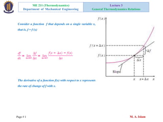
ME 211 (Thermodynamics)
Department of Mechanical Engineering
Lecture 3
General Thermodynamics Relations
Page # 1 M. A. Islam
Consider a function f that depends on a single variable x,
that is, f = f (x)
The derivative of a function f(x) with respect to x represents
the rate of change of f with x.

Lecture 3
Example: The Cp of ideal gases depends on temperature only, and it is expressed as cp(T ) dh(T )/dT.
Determine the cp of air at 300 K, using the enthalpy data from Table A–17 [3]

Lecture 3
Partial derivative
The variation of z(x, y) with x when y is held constant is called
the partial derivative of z with respect to x, and it is expressed as
1) The total differential change (d) of a function and reflects the influence of all variables
2) The partial differential change (𝜕) due to the variation of a single variable
Geometric representation of partial derivative
Examines the dependence of z on only one of the variables

Lecture 3
The fundamental relation for total derivative with partial derivatives
Consider a small portion of the surface z(x, y) and for total differential change in z(x, y) for
simultaneous changes in x and y.
When the independent variables x and y change by ∆ x and
∆ y, respectively, the dependent variable z changes by ∆ z
Geometric representation dz for a function z(x, y)
𝒅𝒛 =
𝝏𝒛
𝝏𝒙 𝒚
𝒅𝒙 +
𝝏𝒛
𝝏𝒚 𝒙
𝒅𝒚

Lecture 3
Example: Total Differential versus Partial Differential:
Consider air at 300 K and 0.86 m3/kg. The state of air changes to 302 K and 0.87 m3/kg as a result
of some disturbance. Using Eq., estimate the change in the pressure of air

ME
211
(Thermodynamics)
Department
of
Mechanical
Engineering
Lecture
3
General
thermodynamics
relation

Lecture 3

Lecture 3
Example: Using the ideal-gas equation of state, verify (a) the cyclic relation and (b) the reciprocity
relation at constant P.

Lecture 3
Maxwell Relations
The equations that relate the partial derivatives of properties P, v, T, and s of a simple compressible
system to each other are called the Maxwell relations.
They are obtained from the four Gibbs equations by exploiting the exactness of the differentials of
thermodynamic properties.
hey are extremely valuable in thermodynamics because they provide
a means of determining
the change in entropy,which cannot be measured directly,by simply
measuring the changes in properties P, v,and T.
Note that the Maxwell relations given above are limited to simple
compressible systems. However, other similar relations can be
written just as easily for nonsimple systems such as those involving
electrical, magnetic, and other effects

Lecture 3
Maxwell relations
𝒅𝑼 = 𝑻𝒅𝑺 − 𝑷𝒅𝑽 −
𝜕𝑃
𝜕𝑆 𝑉
=
𝜕𝑇
𝜕𝑉 𝑆
𝒅𝑯 = 𝑻𝒅𝑺 + 𝑽𝒅𝑷
𝜕𝑇
𝜕𝑃 𝑆
=
𝜕𝑉
𝜕𝑆 𝑃
𝑑𝐹 = − 𝑆𝑑𝑇 − 𝑃𝑑𝑉 −
𝜕𝑆
𝜕𝑉 𝑇
= −
𝜕𝑃
𝜕𝑇 𝑃
𝒅𝑮 = −𝑺𝒅𝑻 + 𝑽𝒅𝑷
−
𝜕𝑆
𝜕𝑃 𝑇
=
𝜕𝑉
𝜕𝑇 𝑃
Coefficient Relations
Consider a function, Z = Z (X, Y), then dZ = M dX + N dY
The coefficients in terms of explicit partial derivatives
𝑴 =
𝝏𝒁
𝝏𝑿 𝒀
and 𝑵 =
𝝏𝒁
𝝏𝒀 𝑿
So,
𝝏𝑴
𝝏𝒀 𝑿
=
𝝏𝑵
𝝏𝑿 𝒀

Lecture 3
For Isobaric process: 𝒅𝑯𝑷 = 𝑻𝒅𝑺𝑷 = 𝜹 𝑸𝒓𝒆𝒗, 𝑷
𝒅𝑯 = 𝑻𝒅𝑺 + 𝑽𝒅𝑷
𝒅𝑯 = (𝑻𝒅𝑺 − 𝑷𝒅𝑽) + 𝑷𝒅𝑽 + 𝑽𝒅𝑷
𝒅𝑯 = 𝒅𝑼 + 𝑷𝒅𝑽 + 𝑽𝒅𝑷
H = U +PV
For Isothermal process: 𝒅𝑭𝑻 = −𝑷 𝒅𝑽𝑻 = δ𝑾𝑻,𝑻𝒐𝒕𝒂𝒍
𝒅𝑭 = − 𝑺𝒅𝑻 − 𝑷𝒅𝑽
𝒅𝑭 = 𝑻𝒅𝑺 − 𝑷𝒅𝑽 − 𝑻𝒅𝑺 − 𝑺𝒅𝑻
𝒅𝑭 = 𝒅𝑼 − 𝑻𝒅𝑺 − 𝑺𝒅𝑻
F = U -TS
The
Helmholtz
Free
energy
The
Enthalpy

Lecture 3
Phase transformation and chemical reaction: 𝛿𝐺𝑇,𝑃 = 𝛿𝑊′
𝑇,
𝑑𝐺 = −𝑆𝑑𝑇 + 𝑉𝑑𝑃
𝑑𝐺 = 𝑇𝑑𝑆 − 𝑃𝑑𝑉 − 𝑃𝑑𝑉 + 𝑉𝑑𝑃 − 𝑇𝑑𝑆 − 𝑇𝑑𝑆 − 𝑆𝑑𝑇
𝑑𝐺 = 𝑑𝑈 + 𝑃𝑑𝑉 + 𝑉𝑑𝑃 − 𝑇𝑑𝑆 − 𝑆𝑑𝑇
G = H -TS = U + PV - TS

Lecture 3
Example: Verify the validity of the last Maxwell relation for steam at 250°C and 300 kPa.

Lecture 3
General relations for du, dh, ds, Cv and Cp
We choose the internal energy to be a function of T and v; that is, u = u(T, v) and take its total
differential

Lecture 3

Lecture 3
The Joule-Thomson Coefficient
 When a fluid passes through a restriction such as a porous plug, a capillary tube, or an ordinary
valve, its pressure decrease
 the enthalpy of the fluid remains approximately constant during such a throttling process
 The fluid may experience a large drop in its temperature as a result of throttling, which forms
the basis of operation for refrigerators and air conditioners.
 The temperature of the fluid may remain unchanged, or it may even increase during a throttling
process

Lecture 3
 The temperature behavior of a fluid during a throttling (h = constant)process is described by the
Joule-Thomson coefficient, defined as
 𝝁 =
𝝏𝑻
𝝏𝑷 𝒉
 The Joule-Thomson coefficient is a measure of the change in temperature with pressure during
a constant-enthalpy process.
Consequences during Throttling process
𝝁
< 𝑻𝒆𝒎𝒑𝒆𝒓𝒂𝒕𝒖𝒓𝒆 𝑰𝒏𝒄𝒓𝒆𝒂𝒔𝒆𝒔
= 𝟎 𝑻𝒆𝒎𝒑𝒆𝒓𝒂𝒕𝒖𝒓𝒆 𝒄𝒐𝒏𝒔𝒕𝒂𝒏𝒕
> 𝑻𝒆𝒎𝒑𝒆𝒓𝒂𝒕𝒖𝒓𝒆 𝒅𝒆𝒄𝒓𝒆𝒂𝒔𝒆𝒔

Lecture 3
The Joule-Thomson coefficient represents the slope of h constant lines on a T-P diagram
Construction of TP Diagram
 Measure temperature and pressure during throttling
processes.
 Repeat the experiment is for different sizes of porous
plugs, each giving a different set of T2 and P2.
 Plot the temperatures against the pressures gives us an h
constant line on a T-P diagramas shown in Figure.

Lecture 3
Repeating the experiment for different sets of inlet pressure and temperature and plotting the results,
a T-P diagram can be constructed for a substance with several h constant lines as in Figure.
The inversion line: Some constant-enthalpy lines on the T-P
diagram pass through a point of zero slope or zero Joule-
Thomson coefficient.
Inversion temperature: The temperature at a point where a
constant-enthalpy line intersects the inversion line.
The maximum inversion temperature: The temperature at
the intersection of the P 0 ine (ordinate) and the upper part of
the inversion line
The slopes of the h constant lines are negative (𝜇 < 0 ) at states to the right of the inversion line and
positive (𝝁 > 𝟎 ) to the left of the inversion line

Lecture 3
Consequences during Throttling
 The temperature of a fluid increases on the right-hand
side of the inversion line (𝑻 ↑, 𝑷 ↓, 𝑫 → , 𝝁 < 𝟎). (process
proceeds along a constant-enthalpy line in the direction of
decreasing pressure, that is, from right to left.)
 The fluid temperature decreases on the left-hand side of
the inversion line (𝑻 ↓, 𝑷 ↑, 𝑫 ← , 𝝁 > 𝟎) .(Process
proceeds along a constant-enthalpy line in the direction of
increasing pressure, that is, from left to write)
Figure: Constant-enthalpy lines of
a substance on a T-P diagram

Lecture 3
 A cooling effect cannot be achieved by throttling unless
the fluid is below its maximum inversion temperature.
 A problem for substances whose maximum inversion
temperature is well below room temperature.
Example: For hydrogen, the maximum inversion temperature is
- 68°C. Thus hydrogen must be cooled below this temperature if
any further cooling is to be achieved by throttling.
A general relation for the Joule-Thomson coefficient
We know, 𝒅𝒉 = 𝑪𝒑𝒅𝑻 + 𝒗 − 𝑻
𝒅𝒗
𝒅𝑷 𝑷
𝒅𝑷
When h = constant, ⇒ 𝝁𝑱𝑻=
𝒅𝑻
𝒅𝑷 𝒉
= −
𝟏
𝑪𝒑
𝒗 − 𝑻
𝒅𝒗
𝒅𝑷 𝑷
𝒅𝑷
Figure: Constant-enthalpy lines of
a substance on a T-P diagram

Lecture 3
Problem: Show that the Joule-Thomson coefficient of an ideal gas is zero.

Lecture 3
Calculating thermodynamic properties such as enthalpy or entropy in terms of other properties
that can be measured, the calculations fall into two broad categories:
1) differences in properties between two different phases
2) Changes within a single homogeneous phase

Lecture 3
Consider a Carnot-cycle heat engine operating across a small temperature difference between
reservoirs at T and T − ∆ T. The corresponding saturation pressures are P and P − ∆P. The Carnot
cycle operates with four steady-state devices. In the high-temperature heat-transfer process, the
working fluid changes from saturated liquid at 1 to saturated vapor at 2, as shown in the two diagrams
of figure.
For reversible heat transfer process
𝑞𝐻 = 𝑇𝑆𝑓𝑔 ; 𝑞𝐿 = (𝑇 − ∆𝑇)𝑆𝑓𝑔 ;
𝑊𝑛𝑒𝑡 = 𝑞𝐻 − 𝑞𝐿 = ∆𝑇𝑆𝑓𝑔
As in figure b, each process is steady and reversible 𝑤 = −𝑣 𝑑𝑃

Lecture 3
Over all, for the four processes in the cycle
𝑊𝑛𝑒𝑡 = 0 +
2
3
𝑣 𝑑𝑃 + 0 +
4
1
𝑣 𝑑𝑃
= −
𝑣2 + 𝑣3
2
𝑃 − ∆𝑃 − 𝑃 −
𝑣1 + 𝑣4
2
𝑃 − ∆𝑃 − 𝑃
= ∆𝑃
𝑣2+𝑣3
2
−
𝑣1+𝑣4
2
= 𝑞𝐻 − 𝑞𝐿 = ∆𝑇𝑆𝑓𝑔
After simplification and rearranging,
∆𝑃
∆𝑇
≈
𝑆𝑓𝑔
𝑣2+𝑣3
2
−
𝑣1+𝑣4
2
In this limit, ∆𝑇 → 0: 𝑣3 → 𝑣2 = 𝑣𝑔; 𝑣4 → 𝑣1 = 𝑣𝑓
lim
∆𝑇→0
∆𝑃
∆𝑇
=
𝑑𝑃𝑠𝑎𝑡
𝑑𝑇
=
𝑆𝑓𝑔
𝑣𝑓𝑔
The heat addition process 1 – 2 is at constant pressure as well as constant temperature
𝒒𝑯 = 𝒉𝒇𝒈 = ∆𝑻𝑺𝒇𝒈
𝒅𝑷𝒔𝒂𝒕
𝒅𝑻
=
𝑺𝒇𝒈
𝒗𝒇𝒈
=
𝒉𝒇𝒈
𝑻𝒗𝒇𝒈
( Clapeyron equation)
 This equation establishes the means to cross from one phase to another in 1st or 2nd law
calculations

Lecture 3
Clapeyron equation for fusion
𝒅𝑷𝒇𝒖𝒔
𝒅𝑻
=
𝑺𝒊𝒇
𝒗𝒊𝒇
=
𝒉𝒊𝒇
𝑻𝒗𝒊𝒇
Clapeyron equation for Sublimation
𝒅𝑷𝑺𝒖𝒃
𝒅𝑻
=
𝑺𝒊𝒈
𝒗𝒊𝒈
=
𝒉𝒊𝒈
𝑻𝒗𝒊𝒈

Lecture 3
Determine the sublimation pressure of water vapor at −60◦C using
data available in the steam tables.

Lecture 3
Exercises
1. Prove the cyclic relation
𝜕𝑧
𝜕𝑥 𝑦
𝜕𝑥
𝜕𝑦 𝑧
𝜕𝑦
𝜕𝑧 𝑥
= - 1

Lecture 3

Thermodynamics Lecture on General Relations and the Joule-Thomson Coefficient

Recommended

Recommended

More Related Content

What's hot

What's hot (20)

Similar to Thermodynamics Lecture on General Relations and the Joule-Thomson Coefficient

Similar to Thermodynamics Lecture on General Relations and the Joule-Thomson Coefficient (20)

Recently uploaded

Recently uploaded (20)

Thermodynamics Lecture on General Relations and the Joule-Thomson Coefficient