SlideShare a Scribd company logo
1 of 18
Download to read offline
Forouzan: Data I II. Physical layer and I 6. Bandwidth Utilization: I I © The McGraw-Hill I
Communications and Media Multiplexing and Companies, 2007
Networking, Fourth Edition Spreading
174 CHAPTER 6 BANDWIDTH UTILIZATION: MULTIPLEXING AND SPREADING
if data rates are not the same, three strategies, or a combination of them, can be used.
We call these three strategies multilevel multiplexing, multiple-slot allocation, and
pulse stuffing.
Multilevel Multiplexing Multilevel multiplexing is a technique used when the data
rate of an input line is a multiple of others. For example, in Figure 6.19, we have two
inputs of 20 kbps and three inputs of 40 kbps. The first two input lines can be multi-
plexed together to provide a data rate equal to the last three. A second level of multi-
plexing can create an output of 160 kbps.
Figure 6.19 Multilevel multiplexing
20 kbps
20 kbps
40 kbps
40 kbps
40 kbps
0 kbps
0 kbps
V
160 kbps
Multiple-Slot Allocation Sometimes it is more efficient to allot more than one slot in
a frame to a single input line. For example, we might have an input line that has a data
rate that is a multiple of another input. In Figure 6.20, the input line with a 50-kbps data
rate can be given two slots in the output. We insert a serial-to-parallel converter in the
line to make two inputs out of one.
Figure 6.20 Multiple-slot multiplexing
25 kbps
50 kbps • 25 kbps
25 kbps •
25 kbps •
25 kbps
The input with a
50-kHz data rate has two
slots in each frame.
• 125 kbps
Pulse Stuffing Sometimes the bit rates of sources are not multiple integers of each
other. Therefore, neither of the above two techniques can be applied. One solution is to
make the highest input data rate the dominant data rate and then add dummy bits to the
input lines with lower rates. This will increase their rates. This technique is called pulse
stuffing, bit padding, or bit stuffing. The idea is shown in Figure 6.21. The input with a
data rate of 46 is pulse-stuffed to increase the rate to 50 kbps. Now multiplexing can
take place.
II. Physical Layer and
Media
6. Bandwidth Utilization:
Multiplexing and
Spreading
SECTION 6.1 MULTIPLEXING 175
Figure 6.21 Pulse stuffing
50 kbps
50 kbps
46 kbps
Frame Synchronizing
The implementation of TDM is not as simple as that of FDM. Synchronization between
the multiplexer and demultiplexer is a major issue. If the multiplexer and the demulti-
plexer are not synchronized, a bit belonging to one channel may be received by the
wrong channel. For this reason, one or more synchronization bits are usually added to
the beginning of each frame. These bits, called framing bits, follow a pattern, frame to
frame, that allows the demultiplexer to synchronize with the incoming stream so that it
can separate the time slots accurately. In most cases, this synchronization information
consists of 1 bit per frame, alternating between 0 and 1, as shown in Figure 6.22.
Figure 6.22 Framing bits
1 o 1
I
Synchronization
pattern
Frame 3
C3 ! B3 ! A3
Frame 2
1
B2 ! A2
•
Frame 1
!
CI |
i
| Al
!
B' in
Example 6.10
We have four sources, each creating 250 characters per second. If the interleaved unit is a character
and 1 synchronizing bit is added to each frame, find (a) the data rate of each source, (b) the duration
of each character in each source, (c) the frame rate, (d) the duration of each frame, (e) the number of
bits in each frame, and (f) the data rate of the link.
Solution
We can answer the questions as follows:
a. The data rate of each source is 250 x 8 = 2000 bps = 2 kbps.
b. Each source sends 250 characters per second; therefore, the duration of a character is 1/250 s,
or 4 ms.
c. Each frame has one character from each source, which means the link needs to send
250 frames per second to keep the transmission rate of each source.
d. The duration of each frame is 1/250 s, or 4 ms. Note that the duration of each frame is the
same as the duration of each character coming from each source.
e. Each frame carries 4 characters and 1 extra synchronizing bit. This means that each frame is
4 x 8 + 1 = 33 bits.
Forouzan: Data I II. Physical Layer and I 6. Bandwidth Utilization: I I © The McGraw-Hill I
Communications and Media Multiplexing and Companies, 2007
Networking, Fourth Edition Spreading
176 CHAPTER 6 BANDWIDTH UTILIZATION: MULTIPLEXING AND SPREADING
f. The link sends 250 frames per second, and each frame contains 33 bits. This means that the
data rate of the link is 250 x 33, or 8250 bps. Note that the bit rate of the link is greater than
the combined bit rates of the four channels. If we add the bit rates of four channels, we get
8000 bps. Because 250 frames are traveling per second and each contains 1 extra bit for
synchronizing, we need to add 250 to the sum to get 8250 bps.
Example 6.11
Two channels, one with a bit rate of 100 kbps and another with a bit rate of 200 kbps, are to be
multiplexed. How this can be achieved? What is the frame rate? What is the frame duration?
What is the bit rate of the link?
Solution
We can allocate one slot to thefirstchannel and two slots to the second channel. Each frame car-
ries 3 bits. The frame rate is 100,000 frames per second because it carries 1 bit from the first
channel. The frame duration is 1/100,000 s, or 10 ms. The bit rate is 100,000 frames/s x 3 bits per
frame, or 300 kbps. Note that because each frame carries 1 bit from thefirstchannel, the bit rate
for the first channel is preserved. The bit rate for the second channel is also preserved because
each frame carries 2 bits from the second channel.
Digital Signal Service
Telephone companies implement TDM through a hierarchy of digital signals, called
digital signal (DS) service or digital hierarchy. Figure 6.23 shows the data rates sup-
ported by each level.
Figure 6.23 Digital hierarchy
• A DS-0 service is a single digital channel of 64 kbps.
• DS-1 is a 1.544-Mbps service; 1.544 Mbps is 24 times 64 kbps plus 8 kbps of
overhead. It can be used as a single service for 1.544-Mbps transmissions, or it can
be used to multiplex 24 DS-0 channels or to carry any other combination desired
by the user that can fit within its 1.544-Mbps capacity.
• DS-2 is a 6.312-Mbps service; 6.312 Mbps is 96 times 64 kbps plus 168 kbps of
overhead. It can be used as a single service for 6.312-Mbps transmissions; or it can
Forouzan: Data
Communications and
Networking, Fourth Edition
II. Physical Layer and
Media
6. Bandwidth Utilization:
Multiplexing and
Spreading
©The McGraw-Hill
Companies, 2007
SECTION 6.1 MULTIPLEXING 177
be used to multiplex 4 DS-1 channels, 96 DS-0 channels, or a combination of these
service types.
• DS-3 is a 44.376-Mbps service; 44.376 Mbps is 672 times 64 kbps plus 1.368 Mbps
of overhead. It can be used as a single service for 44.376-Mbps transmissions; or it
can be used to multiplex 7 DS-2 channels, 28 DS-1 channels, 672 DS-0 channels,
or a combination of these service types.
• DS-4 is a 274.176-Mbps service; 274.176 is 4032 times 64 kbps plus 16.128 Mbps of
overhead. It can be used to multiplex 6 DS-3 channels, 42 DS-2 channels, 168 DS-1
channels, 4032 DS-0 channels, or a combination of these service types.
DS-0, DS-1, and so on are the names of services. To implement those services, the tele-
phone companies use T lines (T-l to T-4). These are lines with capacities precisely
matched to the data rates of the DS-1 to DS-4 services (see Table 6.1). So far only T-l
and T-3 lines are commercially available.
Table 6.1 DS and T line rates
Service Line Rate (Mbps) Voice Channels
DS-1 T-l 1.544 24
DS-2 T-2 6.312 96
DS-3 T-3 44.736 672
DS-4 T-4 274.176 4032
The T-l line is used to implement DS-1; T-2 is used to implement DS-2; and so on.
As you can see from Table 6.1, DS-0 is not actually offered as a service, but it has been
defined as a basis for reference purposes.
T Lines for Analog Transmission
T lines are digital lines designed for the transmission of digital data, audio, or video.
However, they also can be used for analog transmission (regular telephone connec-
tions), provided the analog signals are first sampled, then time-division multiplexed.
The possibility of using T lines as analog carriers opened up a new generation of
services for the telephone companies. Earlier, when an organization wanted 24 separate
telephone lines, it needed to run 24 twisted-pair cables from the company to the central
exchange. (Remember those old movies showing a busy executive with 10 telephones
lined up on his desk? Or the old office telephones with a big fat cable running from
them? Those cables contained a bundle of separate lines.) Today, that same organization
can combine the 24 lines into one T-l line and run only the T-l line to the exchange.
Figure 6.24 shows how 24 voice channels can be multiplexed onto one T-l line. (Refer
to Chapter 5 for PCM encoding.)
The T-l Frame As noted above, DS-1 requires 8 kbps of overhead. To understand how
this overhead is calculated, we must examine the format of a 24-voice-channel frame.
The frame used on a T-l line is usually 193 bits divided into 24 slots of 8 bits each
plus 1 extra bit for synchronization (24 x 8 + 1 = 193); see Figure 6.25. In other words,
T Lines
Forouzan: Data I II. Physical Layer and I 6. Bandwidth Utilization: I I © The McGraw-Hill
Communications and Media Multiplexing and Companies, 2007
Networking, Fourth Edition Spreading
178 CHAPTER 6 BANDWIDTH UTILIZATION: MULTIPLEXING AND SPREADING
Figure 6.24 T-l linefor multiplexing telephone lines
/Sampling at 8000 samples/sN
V using 8 bits per sample J
T-l line 1.544 Mbps
24 x 64 kbps + 8 kbps overhead
each slot contains one signal segment from each channel; 24 segments are interleaved
in one frame. If a T-l line carries 8000 frames, the data rate is 1.544 Mbps (193 x 8000 =
1.544 Mbps)—the capacity of the line.
E Lines
Europeans use a version of T lines called E lines. The two systems are conceptually iden-
tical, but their capacities differ. Table 6.2 shows the E lines and their capacities.
Forouzan: Data I II. Physical Layer and I 6. Bandwidth Utilization: I I © The McGraw-Hill
Communications and Media Multiplexing and Companies, 2007
Networking, Fourth Edition Spreading
SECTION 6.1 MULTIPLEXING 179
Table 6.2 E line rates
Line Rate (Mbps) Voice Channels
E-1 2.048 30
E-2 8.448 120
E-3 34.368 480
E-4 139.264 1920
More Synchronous TDM Applications
Some second-generation cellular telephone companies use synchronous TDM. For
example, the digital version of cellular telephony divides the available bandwidth into
30-kHz bands. For each band, TDM is applied so that six users can share the band. This
means that each 30-kHz band is now made of six time slots, and the digitized voice sig-
nals of the users are inserted in the slots. Using TDM, the number of telephone users in
each area is now 6 times greater. We discuss second-generation cellular telephony in
Chapter 16.
Statistical Time-Division Multiplexing
As we saw in the previous section, in synchronous TDM, each input has a reserved slot
in the output frame. This can be inefficient if some input lines have no data to send. In
statistical time-division multiplexing, slots are dynamically allocated to improve band-
width efficiency. Only when an input line has a slot's worth of data to send is it given a
slot in the output frame. In statistical multiplexing, the number of slots in each frame is
less than the number of input lines. The multiplexer checks each input line in round-
robin fashion; it allocates a slot for an input line if the line has data to send; otherwise,
it skips the line and checks the next Line.
Figure 6.26 shows a synchronous and a statistical TDM example. In the former,
some slots are empty because the corresponding line does not have data to send. In
the latter, however, no slot is left empty as long as there are data to be sent by any
input line.
Addressing
Figure 6.26 also shows a major difference between slots in synchronous TDM and
statistical TDM. An output slot in synchronous TDM is totally occupied by data; in
statistical TDM, a slot needs to carry data as well as the address of the destination.
In synchronous TDM, there is no need for addressing; synchronization and preassigned
relationships between the inputs and outputs serve as an address. We know, for exam-
ple, that input 1 always goes to input 2. If the multiplexer and the demultiplexer are
synchronized, this is guaranteed. In statistical multiplexing, there is no fixed relation-
ship between the inputs and outputs because there are no preassigned or reserved
slots. We need to include the address of the receiver inside each slot to show where it
is to be delivered. The addressing in its simplest form can be n bits to define N different
output lines with n = log2 N. For example, for eight different output lines, we need a
3-bit address.
Forouzan: Data I II. Physical Layer and I 6. Bandwidth Utilization: I I © The McGraw-Hill I
Communications and Media Multiplexing and Companies, 2007
Networking, Fourth Edition Spreading
180 CHAPTER 6 BANDWIDTH UTILIZATION: MULTIPLEXING AND SPREADING
Figure 6.26 TDM slot comparison
a. Synchronous TDM
Line A 1 A1 r
LineB—I H2 H~~Bl [
Line C
Line D —I P2
Line E
b. Statistical TDM
Slot Size
Since a slot carries both data and an address in statistical TDM, the ratio of the data size
to address size must be reasonable to make transmission efficient. For example, it
would be inefficient to send 1 bit per slot as data when the address is 3 bits. This would
mean an overhead of 300 percent. In statistical TDM, a block of data is usually many
bytes while the address is just a few bytes.
No Synchronization Bit
There is another difference between synchronous and statistical TDM, but this time it is
at the frame level. The frames in statistical TDM need not be synchronized, so we do not
need synchronization bits.
Bandwidth
In statistical TDM, the capacity of the link is normally less than the sum of the capaci-
ties of each channel. The designers of statistical TDM define the capacity of the link
based on the statistics of the load for each channel. If on average only x percent of the
input slots are filled, the capacity of the link reflects this. Of course, during peak times,
some slots need to wait.
6.2 SPREAD SPECTRUM
Multiplexing combines signals from several sources to achieve bandwidth efficiency; the
available bandwidth of a link is divided between the sources. In spread spectrum (SS), we
also combine signals from different sources to fit into a larger bandwidth, but our goals
6. Bandwidth Utilization:
Multiplexing and
Spreading
SECTION 6.2 SPREAD SPECTRUM 181
are somewhat different. Spread spectrum is designed to be used in wireless applications
(LANs and WANs). In these types of applications, we have some concerns that outweigh
bandwidth efficiency. In wireless applications, all stations use air (or a vacuum) as the
medium for communication. Stations must be able to share this medium without intercep-
tion by an eavesdropper and without being subject to jamming from a malicious intruder
(in military operations, for example).
To achieve these goals, spread spectrum techniques add redundancy; they spread
the original spectrum needed for each station. If the required bandwidth for each station
is B, spread spectrum expands it to B s s , such that B s s » B. The expanded bandwidth
allows the source to wrap its message in a protective envelope for a more secure trans-
mission. An analogy is the sending of a delicate, expensive gift. We can insert the gift in
a special box to prevent it from being damaged during transportation, and we can use a
superior delivery service to guarantee the safety of the package.
Figure 6.27 shows the idea of spread spectrum. Spread spectrum achieves its goals
through two principles:
1. The bandwidth allocated to each station needs to be, by far, larger than what is
needed. This allows redundancy.
2. The expanding of the original bandwidth B to the bandwidth Bss must be done by a
process that is independent of the original signal. In other words, the spreading
process occurs after the signal is created by the source.
Figure 6.27 Spread spectrum
Spreading
Spreading
process
I
Spreading
code
After the signal is created by the source, the spreading process uses a spreading
code and spreads the bandwidth. The figure shows the original bandwidth B and the
spreaded bandwidth Bss. The spreading code is a series of numbers that look random,
but are actually a pattern.
There are two techniques to spread the bandwidth: frequency hopping spread spec-
trum (FHSS) and direct sequence spread spectrum (DSSS).
Frequency Hopping Spread Spectrum (FHSS)
The frequency hopping spread spectrum (FHSS) technique uses M different carrier
frequencies that are modulated by the source signal. At one moment, the signal modu-
lates one carrier frequency; at the next moment, the signal modulates another carrier
Forouzan: Data I II. Physical Layer and I 6. Bandwidth Utilization: I I © The McGraw-Hill I ^
Communications and Media Multiplexing and Companies, 2007
Networking, Fourth Edition Spreading
182 CHAPTER 6 BANDWIDTH UTILIZATION: MULTIPLEXING AND SPREADING
frequency. Although the modulation is done using one carrier frequency at a time,
M frequencies are used in the long run. The bandwidth occupied by a source after
spreading is fipnss > : >
Figure 6.28 shows the general layout for FHSS. A pseudorandom code generator,
called pseudorandom noise (PN), creates afc-bitpattern for every hopping period T^.
The frequency table uses the pattern to find the frequency to be used for this hopping
period and passes it to the frequency synthesizer. The frequency synthesizer creates a
carrier signal of that frequency, and the source signal modulates the carrier signal.
Figure 6.28 Frequency hopping spread spectrum (FHSS)
Original
signal
.2 3'
Modulator
_ Spread
signal
Frequency
synthesizer
Frequency table
Suppose we have decided to have eight hopping frequencies. This is extremely low
for real applications and is just for illustration. In this case, M is 8 and k is 3. The pseudo-
random code generator will create eight different 3-bit patterns. These are mapped to
eight different frequencies in the frequency table (see Figure 6.29).
Figure 6.29 Frequency selection in FHSS
First-hop frequency
fe-bit patterns
ioi in ooi ooo oio no on 100
First selection
it-bit
000
001
010
on
100
-101
110
111
Frequency
200 kH?
300 kHz
400 kHz
500 kHz
600 kHz
700 kHz -
800 kHz
900 kHz
Frequency table
Forouzan: Data I II. Physical Layer and I 6. Bandwidth Utilization: I I © The McGraw-Hill
Communications and Media Multiplexing and Companies, 2007
Networking, Fourth Edition Spreading
SECTION 6.2 SPREAD SPECTRUM 183
The pattern for this station is 101, 111, 001, 000, 010, 011, 100. Note that the pat-
tern is pseudorandom it is repeated after eight hoppings. This means that at hopping
period 1, the pattern is 101. The frequency selected is 700 kHz; the source signal mod-
ulates this carrier frequency. The secondfc-bitpattern selected is 111, which selects the
900-kHz carrier; the eighth pattern is 100, the frequency is 600 kHz. After eight hop-
pings, the pattern repeats, starting from 101 again. Figure 6.30 shows how the signal hops
around from carrier to carrier. We assume the required bandwidth of the original signal
is 100 kHz.
Figure 6.30 FHSS cycles
Carrier
frequencies
(kHz)
900
800
700
600
500
400
300
200
Cycle 1
~A IBB
• M M * ;
- Q -
Cycle 2
•
•
1 2 3 4 5 6 7 8 9 10 11 12 13 14 15 16 Hop
periods
It can be shown that this scheme can accomplish the previously mentioned goals.
If there are many fc-bit patterns and the hopping period is short, a sender and receiver
can have privacy. If an intruder tries to intercept the transmitted signal, she can only
access a small piece of data because she does not know the spreading sequence to
quickly adapt herself to the next hop. The scheme has also an antijamming effect. A
malicious sender may be able to send noise to jam the signal for one hopping period
(randomly), but not for the whole period.
Bandwidth Sharing
If the number of hopping frequencies is M, we can multiplex M channels into one by using
the same B s s bandwidth. This is possible because a station uses just one frequency in each
hopping period; M - 1 other frequencies can be used by other M - 1 stations. In other
words, M different stations can use the same Bss if an appropriate modulation technique
such as multiple FSK (MFSK) is used. FHSS is similar to FDM, as shown in Figure 6.31.
Figure 6.31 shows an example of four channels using F D M and four channels
using FHSS. In FDM, each station uses 1/M of the bandwidth, but the allocation is
fixed; in FHSS, each station uses 1/M of the bandwidth, but the allocation changes hop
to hop.
Forouzan: Data I II. Physical Layer and I 6. Bandwidth Utilization: I I © The McGraw-Hill I
Communications and Media Multiplexing and Companies, 2007
Networking, Fourth Edition Spreading
184 CHAPTER 6 BANDWIDTH UTILIZATION: MULTIPLEXING AND SPREADING
Figure 6.31 Bandwidth sharing
Direct Sequence Spread Spectrum
The direct sequence spread spectrum (DSSS) technique also expands the bandwidth
of the original signal, but the process is different. In DSSS, we replace each data bit
with n bits using a spreading code. In other words, each bit is assigned a code of n bits,
called chips, where the chip rate is n times that of the data bit. Figure 6.32 shows the
concept of DSSS.
Figure 6.32 DSSS
Original
signal
Modulator
Spread
signal
Chips generator
As an example, let us consider the sequence used in a wireless LAN, the famous
Barker sequence where n is 11. We assume that the original signal and the chips in the
chip generator use polar NRZ encoding. Figure 6.33 shows the chips and the result of
multiplying the original data by the chips to get the spread signal.
In Figure 6.33, the spreading code is 11 chips having the pattern 10110111000 (in
this case). If the original signal rate is N, the rate of the spread signal is 1 IN. This
means that the required bandwidth for the spread signal is 11 times larger than the
bandwidth of the original signal. The spread signal can provide privacy if the intruder
does not know the code. It can also provide immunity against interference if each sta-
tion uses a different code.
6. Bandwidth Utilization:
Multiplexing and
Spreading
SECTION 6.4 KEY TERMS 185
Figure 6.33 DSSS example
Original
signal
Spreading
code
Spread
signal
• 1
1 0 1 1 0 1 1 I
"
1
1
—
1
1
0 0 0 j a i i o i i i
1 P I 1
U » 0 1 0 1 1 0 1 1 1
11—11
0 0 0]
1
u u
"1 I
— 1
1 u •
n n
u u
II II
1
1
1
1
U J II '11', U Li 1
1
Bandwidth Sharing
Can we share a bandwidth in DSSS as we did in FHSS? The answer is no and yes. If we
use a spreading code that spreads signals (from different stations) that cannot be combined
and separated, we cannot share a bandwidth. For example, as we will see in Chapter 14,
some wireless LANs use DSSS and the spread bandwidth cannot be shared. However, if
we use a special type of sequence code that allows the combining and separating of spread
signals, we can share the bandwidth. As we will see in Chapter 16, a special spreading code
allows us to use DSSS in cellular telephony and share a bandwidth between several users.
6.3 RECOMMENDED READING
For more details about subjects discussed in this chapter, we recommend the following
books. The items in brackets [...] refer to the reference list at the end of the text.
Books
Multiplexing is elegantly discussed in Chapters 19 of [Pea92]. [CouOl] gives excellent
coverage of TDM and FDM in Sections 3.9 to 3.11. More advanced materials can be
found in [Ber96]. Multiplexing is discussed in Chapter 8 of [Sta04]. A good coverage of
spread spectrum can be found in Section 5.13 of [CouOl] and Chapter 9 of [Sta04].
6.4 KEY TERMS
analog hierarchy digital signal (DS) service
Barker sequence direct sequence spread spectrum (DSSS)
channel E line
chip framing bit
demultiplexer (DEMUX) frequency hopping spread spectrum
dense WDM (DWDM) (FSSS)
Forouzan: Data
Communications and
Networking, Fourth Edition
II. Physical Layer and
Media
6. Bandwidth Utilization:
Multiplexing and
Spreading
©The McGraw-Hill
Companies, 2007
186 CHAPTER 6 BANDWIDTH UTILIZATION: MULTIPLEXING AND SPREADING
• Bandwidth utilization is the use of available bandwidth to achieve specific goals.
Efficiency can be achieved by using multiplexing; privacy and antijamming can be
achieved by using spreading.
• Multiplexing is the set of techniques that allows the simultaneous transmission of
multiple signals across a single data link. In a multiplexed system, n lines share the
bandwidth of one link. The word link refers to the physical path. The word channel
refers to the portion of a link that carries a transmission.
• There are three basic multiplexing techniques: frequency-division multiplexing,
wavelength-division multiplexing, and time-division multiplexing. The first two are
techniques designed for analog signals, the third, for digital signals
• Frequency-division multiplexing (FDM) is an analog technique that can be applied
when the bandwidth of a link (in hertz) is greater than the combined bandwidths of
the signals to be transmitted.
• Wavelength-division multiplexing (WDM) is designed to use the high bandwidth
capability of fiber-optic cable. WDM is an analog multiplexing technique to com-
bine optical signals.
• Time-division multiplexing (TDM) is a digital process that allows several connec-
tions to share the high bandwidth of a link. TDM is a digital multiplexing technique
for combining several low-rate channels into one high-rate one.
LI We can divide TDM into two different schemes: synchronous or statistical. In syn-
chronous TDM, each input connection has an allotment in the output even if it is
not sending data. In statistical TDM, slots are dynamically allocated to improve
bandwidth efficiency.
• In spread spectrum (SS), we combine signals from different sources to fit into a
larger bandwidth. Spread spectrum is designed to be used in wireless applications
in which stations must be able to share the medium without interception by an
eavesdropper and without being subject to jamming from a malicious intruder.
• The frequency hopping spread spectrum (FHSS) technique uses M different carrier
frequencies that are modulated by the source signal. At one moment, the signal
frequency-division multiplexing (FDM)
group
guard band
hopping period
interleaving
jumbo group
link
master group
multilevel multiplexing
multiple-slot multiplexing
multiplexer (MUX)
multiplexing
pseudorandom code generator
pseudorandom noise (PN)
pulse stuffing
spread spectrum (SS)
statistical TDM
supergroup
synchronous TDM
T line
time-division multiplexing (TDM)
wavelength-division multiplexing (WDM)
6.5 SUMMARY
Forouzan: Data
Communications and
Networking, Fourth Edition
II. Physical Layer and
Media
6. Bandwidth Utilization:
Multiplexing and
Spreading
©The McGraw-Hill
Ccmpanies, 2007
SECTION 6.6 PRACTICE SET 187
modulates one carrier frequency; at the next moment, the signal modulates another
carrier frequency.
• The direct sequence spread spectrum (DSSS) technique expands the bandwidth of
a signal by replacing each data bit with n bits using a spreading code. In other words,
each bit is assigned a code of n bits, called chips.
Review Questions
1. Describe the goals of multiplexing.
2. List three main multiplexing techniques mentioned in this chapter.
3. Distinguish between a link and a channel in multiplexing.
4. Which of the three multiplexing techniques is (are) used to combine analog signals?
Which of the three multiplexing techniques is (are) used to combine digital signals?
5. Define the analog hierarchy used by telephone companies and list different levels
of the hierarchy.
6. Define the digital hierarchy used by telephone companies and list different levels
of the hierarchy.
7. Which of the three multiplexing techniques is common for fiber optic links?
Explain the reason.
8. Distinguish between multilevel TDM, multiple slot TDM, and pulse-stuffed TDM.
9. Distinguish between synchronous and statistical TDM.
10. Define spread spectrum and its goal. List the two spread spectrum techniques dis-
cussed in this chapter.
11. Define FHSS and explain how it achieves bandwidth spreading.
12. Define DSSS and explain how it achieves bandwidth spreading.
Exercises
13. Assume that a voice channel occupies a bandwidth of 4 kHz. We need to multiplex
10 voice channels with guard bands of 500 Hz using FDM. Calculate the required
bandwidth.
14. We need to transmit 100 digitized voice channels using a pass-band channel of
20 KHz. What should be the ratio of bits/Hz if we use no guard band?
15. In the analog hierarchy of Figure 6.9, find the overhead (extra bandwidth for guard
band or control) in each hierarchy level (group, supergroup, master group, and
jumbo group).
16. We need to use synchronous TDM and combine 20 digital sources, each of 100 Kbps.
Each output slot carries 1 bit from each digital source, but one extra bit is added to
each frame for synchronization. Answer the following questions:
a. What is the size of an output frame in bits?
b. What is the output frame rate?
6.6 PRACTICE SET
Forouzan: Data
Communications and
Networking, Fourth Edition
II. Physical Layer and
Media
6. Bandwidth Utilization:
Multiplexing and
Spreading
©The McGraw-Hill
Companies, 2007
188 CHAPTER 6 BANDWIDTH UTILIZATION: MULTIPLEXING AND SPREADING
c. What is the duration of an output frame?
d. What is the output data rate?
e. What is the efficiency of the system (ratio of useful bits to the total bits).
17. Repeat Exercise 16 if each output slot carries 2 bits from each source.
1.8. We have 14 sources, each creating 500 8-bit characters per second. Since only some
of these sources are active at any moment, we use statistical TDM to combine these
sources using character interleaving. Each frame carries 6 slots at a time, but we need
to add four-bit addresses to each slot. Answer the following questions:
a. What is the size of an output frame in bits?
b. What is the output frame rate?
c. What is the duration of an output frame?
d. What is the output data rate?
19. Ten sources, six with a bit rate of 200 kbps and four with a bit rate of 400 kbps are
to be combined using multilevel TDM with no synchronizing bits. Answer the fol-
lowing questions about the final stage of the multiplexing:
a. What is the size of a frame in bits?
b. What is the frame rate?
c. What is the duration of a frame?
d. What is the data rate?
20. Four channels, two with a bit rate of 200 kbps and two with a bit rate of 150 kbps, are
to be multiplexed using multiple slot TDM with no synchronization bits. Answer
the following questions:
a. What is the size of a frame in bits?
b. What is the frame rate?
c. What is the duration of a frame?
d. What is the data rate?
21. Two channels, one with a bit rate of 190 kbps and another with a bit rate of 180 kbps,
are to be multiplexed using pulse stuffing TDM with no synchronization bits. Answer
the following questions:
a. What is the size of a frame in bits?
b. What is the frame rate?
c. What is the duration of a frame?
d. What is the data rate?
22. Answer the following questions about a T-l line:
a. What is the duration of a frame?
b. What is the overhead (number of extra bits per second)?
23. Show the contents of the five output frames for a synchronous TDM multiplexer
that combines four sources sending the following characters. Note that the characters
are sent in the same order that they are typed. The third source is silent.
a. Source 1 message: HELLO
b. Source 2 message: HI
6. Bandwidth Utilization:
Multiplexing and
Spreading
SECTION 6.6 PRACTICE SET 189
c. Source 3 message:
d. Source 4 message: B Y E
24. Figure 6.34 shows a multiplexer in a synchronous TDM system. Each output slot is
only 10 bits long (3 bits taken from each input plus 1 framing bit). What is the output
stream? The bits arrive at the multiplexer as shown by the arrows.
Figure 6.34 Exercise 24
101110111101
11111110000
1010000001111
Frame of 10 bits
25. Figure 6.35 shows a demultiplexer in a synchronous TDM. If the input slot is 16 bits
long (no framing bits), what is the bit stream in each output? The bits arrive at the
demultiplexer as shown by the arrows.
Figure 6.35 Exercise 25
10100000 1010101010100001 0111000001111000
26. Answer the following questions about the digital hierarchy in Figure 6.23:
a. What is the overhead (number of extra bits) in the DS-1 service?
b. What is the overhead (number of extra bits) in the DS-2 service?
c. What is the overhead (number of extra bits) in the DS-3 service?
d. What is the overhead (number of extra bits) in the DS-4 service?
27. What is the minimum number of bits in a PN sequence if we use FHSS with a
channel bandwidth of B = 4 KHz and B s s = 100 KHz?
28. An FHSS system uses a 4-bit PN sequence. If the bit rate of the PN is 64 bits per
second, answer the following questions:
a. What is the total number of possible hops?
b. What is the time needed to finish a complete cycle of PN?
Forouzan: Data
Communications and
Networking, Fourth Edition
II. Physical Layer and
Media
6. Bandwidth Utilization:
Multiplexing and
Spreading
© The McGraw-Hill
Companies. 2007
190 CHAPTER 6 BANDWIDTH UTILIZATION: MULTIPLEXING AND SPREADING
29. A pseudorandom number generator uses the following formula to create a random
series:
In which Ns defines the current random number and N i + 1 defines the next random
number. The term mod means the value of the remainder when dividing (5 + 7Nj)
by 17.
30. We have a digital medium with a data rate of 10 Mbps. How many 64-kbps voice
channels can be carried by this medium if we use DSSS with the Barker sequence?
N w =(5 + 7Nj)mod 17-1
Forouzan: Data
Communications and
II. Physical Layer and
Media
7. Transmission Media © The McGraw-Hill
Companies, 2007
Transmission Media
We discussed many issues related to the physical layer in/Thapters 3 through 6. In this
chapter, discuss transmission media. Transmission media are actually located below
the physicaKlayer and are directly controlled by the physical layer. You could say that
transmission media belong to layer zero. Figure l.l/hows the position of transmission
media in relation to the physical layer.
Figure 7.1 Transmissiorhnedium andphysical lAyer
Sender Physical layer Physical layer Receiver
Trai fission medium
Cable*
A transmission medium c/n be broadly denied as anything that can carry infor-
mation from a source to a destination. For example>tfie transmission medium for two
people having a dinner conversation is the air. The aincan also be used to convey the
message in a smoke signayor semaphore. For a writterKmessage, the transmission
medium might be a mail ramier, a truck, or an airplane.
In data communications the definition of the informationSmd the transmission
medium is more specific/The transmission medium is usually free sp&re, metallic cable,
or fiber-optic cable. The information is usually a signal that is the result Orva conversion
of data from another /orm.
The use of long-distance communication using electric signals started with the
invention of the telegraph by Morse in the 19th century. Communication by telegraph
was slow and dependent on a metallic medium.
Extending the range of the human voice became possible when the telephone was
invented in 1869. Telephone communication at that time also needed a metallic medium
to carry the electric signals that were the result of a conversion from the human voice.
191

More Related Content

What's hot

Time Division Multiplexing
Time Division MultiplexingTime Division Multiplexing
Time Division MultiplexingSpandit Lenka
 
Point to-point and point-to multipoint wireless connectivity
Point to-point and point-to multipoint wireless connectivityPoint to-point and point-to multipoint wireless connectivity
Point to-point and point-to multipoint wireless connectivitynikhiltech
 
Digital Communication: Information Theory
Digital Communication: Information TheoryDigital Communication: Information Theory
Digital Communication: Information TheoryDr. Sanjay M. Gulhane
 
100 Interview Question in Wireless Communication Industry
100 Interview Question in  Wireless Communication Industry100 Interview Question in  Wireless Communication Industry
100 Interview Question in Wireless Communication IndustryVARUN KUMAR
 
Transmission media ppt
Transmission media pptTransmission media ppt
Transmission media pptShubham Singh
 
Comparative Analysis of Distance Vector Routing & Link State Protocols
Comparative Analysis of Distance Vector Routing & Link State ProtocolsComparative Analysis of Distance Vector Routing & Link State Protocols
Comparative Analysis of Distance Vector Routing & Link State ProtocolsEast West University
 
Packet Tracer: Routing protocols EIGRP and OSPF
Packet Tracer: Routing protocols EIGRP and OSPFPacket Tracer: Routing protocols EIGRP and OSPF
Packet Tracer: Routing protocols EIGRP and OSPFRafat Khandaker
 
Transmission impairments(presentation)
Transmission impairments(presentation)Transmission impairments(presentation)
Transmission impairments(presentation)Vivek Kumar
 
Chap 05
Chap 05Chap 05
Chap 05IGNOU
 

What's hot (20)

HDLC
HDLCHDLC
HDLC
 
Time Division Multiplexing
Time Division MultiplexingTime Division Multiplexing
Time Division Multiplexing
 
transport layer
transport layertransport layer
transport layer
 
Switching systems lecture1
Switching  systems lecture1Switching  systems lecture1
Switching systems lecture1
 
Chapter 6
Chapter 6Chapter 6
Chapter 6
 
Point to-point and point-to multipoint wireless connectivity
Point to-point and point-to multipoint wireless connectivityPoint to-point and point-to multipoint wireless connectivity
Point to-point and point-to multipoint wireless connectivity
 
Digital Communication: Information Theory
Digital Communication: Information TheoryDigital Communication: Information Theory
Digital Communication: Information Theory
 
Sonet
SonetSonet
Sonet
 
100 Interview Question in Wireless Communication Industry
100 Interview Question in  Wireless Communication Industry100 Interview Question in  Wireless Communication Industry
100 Interview Question in Wireless Communication Industry
 
Bandwidth utilization
Bandwidth utilizationBandwidth utilization
Bandwidth utilization
 
Transmission media ppt
Transmission media pptTransmission media ppt
Transmission media ppt
 
Comparative Analysis of Distance Vector Routing & Link State Protocols
Comparative Analysis of Distance Vector Routing & Link State ProtocolsComparative Analysis of Distance Vector Routing & Link State Protocols
Comparative Analysis of Distance Vector Routing & Link State Protocols
 
TCP IP Addressing
TCP IP AddressingTCP IP Addressing
TCP IP Addressing
 
Packet Tracer: Routing protocols EIGRP and OSPF
Packet Tracer: Routing protocols EIGRP and OSPFPacket Tracer: Routing protocols EIGRP and OSPF
Packet Tracer: Routing protocols EIGRP and OSPF
 
Transmission impairments(presentation)
Transmission impairments(presentation)Transmission impairments(presentation)
Transmission impairments(presentation)
 
Mobile computing unit 1
Mobile computing unit 1Mobile computing unit 1
Mobile computing unit 1
 
Chapter 12
Chapter 12Chapter 12
Chapter 12
 
Chap 05
Chap 05Chap 05
Chap 05
 
Network layer tanenbaum
Network layer tanenbaumNetwork layer tanenbaum
Network layer tanenbaum
 
Chapter 3: Data & Signals
Chapter 3: Data & SignalsChapter 3: Data & Signals
Chapter 3: Data & Signals
 

Similar to 3510Chapter6Part2 (1).pdf

Similar to 3510Chapter6Part2 (1).pdf (20)

BANDWIDTH UTILIZATION
BANDWIDTH UTILIZATIONBANDWIDTH UTILIZATION
BANDWIDTH UTILIZATION
 
Mux ppt unit 2 data comm
Mux ppt unit 2 data commMux ppt unit 2 data comm
Mux ppt unit 2 data comm
 
Ch 06
Ch 06Ch 06
Ch 06
 
Multiplexing
MultiplexingMultiplexing
Multiplexing
 
Ch6 1 Data communication and networking by neha g. kurale
Ch6 1 Data communication and networking by neha g. kuraleCh6 1 Data communication and networking by neha g. kurale
Ch6 1 Data communication and networking by neha g. kurale
 
Ch06 multiplexing and ss
Ch06 multiplexing and ssCh06 multiplexing and ss
Ch06 multiplexing and ss
 
Ch06
Ch06Ch06
Ch06
 
ch6_1_v1.ppt
ch6_1_v1.pptch6_1_v1.ppt
ch6_1_v1.ppt
 
ch6_1_v1.ppt
ch6_1_v1.pptch6_1_v1.ppt
ch6_1_v1.ppt
 
multiplexing and spreading bandwidth utilization
multiplexing and spreading  bandwidth utilizationmultiplexing and spreading  bandwidth utilization
multiplexing and spreading bandwidth utilization
 
ch6_1_v1.ppt
ch6_1_v1.pptch6_1_v1.ppt
ch6_1_v1.ppt
 
ch6_1_v1.ppt
ch6_1_v1.pptch6_1_v1.ppt
ch6_1_v1.ppt
 
Multiplexing l7
Multiplexing l7Multiplexing l7
Multiplexing l7
 
Multiplexing and Spreading-1.pdf
Multiplexing and Spreading-1.pdfMultiplexing and Spreading-1.pdf
Multiplexing and Spreading-1.pdf
 
Lecture-6 Data Communication ~www.fida.com.bd
Lecture-6 Data Communication ~www.fida.com.bdLecture-6 Data Communication ~www.fida.com.bd
Lecture-6 Data Communication ~www.fida.com.bd
 
Multiplexing and spreading
Multiplexing and spreadingMultiplexing and spreading
Multiplexing and spreading
 
Chuong 06(multiplexing)
Chuong 06(multiplexing)Chuong 06(multiplexing)
Chuong 06(multiplexing)
 
COMPUTER NETWORK - Chapter - 3
COMPUTER NETWORK - Chapter - 3COMPUTER NETWORK - Chapter - 3
COMPUTER NETWORK - Chapter - 3
 
Chapter 6 bandwidth utilization -multiplexing and spreading_computer_network
Chapter 6   bandwidth utilization -multiplexing and spreading_computer_networkChapter 6   bandwidth utilization -multiplexing and spreading_computer_network
Chapter 6 bandwidth utilization -multiplexing and spreading_computer_network
 
Ch06
Ch06Ch06
Ch06
 

More from SoyallRobi

you_can_find_some_TDM_related_math.pdf
you_can_find_some_TDM_related_math.pdfyou_can_find_some_TDM_related_math.pdf
you_can_find_some_TDM_related_math.pdfSoyallRobi
 
Assignment #4-Ch5-6-7-8-Data Communications.pdf
Assignment #4-Ch5-6-7-8-Data Communications.pdfAssignment #4-Ch5-6-7-8-Data Communications.pdf
Assignment #4-Ch5-6-7-8-Data Communications.pdfSoyallRobi
 
_Pulse-Modulation-Techniqnes.pdf
_Pulse-Modulation-Techniqnes.pdf_Pulse-Modulation-Techniqnes.pdf
_Pulse-Modulation-Techniqnes.pdfSoyallRobi
 
_Pulse-Modulation-Systems.pdf
_Pulse-Modulation-Systems.pdf_Pulse-Modulation-Systems.pdf
_Pulse-Modulation-Systems.pdfSoyallRobi
 
_Amplitude-Modulated-Systmes.pdf
_Amplitude-Modulated-Systmes.pdf_Amplitude-Modulated-Systmes.pdf
_Amplitude-Modulated-Systmes.pdfSoyallRobi
 
_Amplitude-Modulated-Systems.pdf
_Amplitude-Modulated-Systems.pdf_Amplitude-Modulated-Systems.pdf
_Amplitude-Modulated-Systems.pdfSoyallRobi
 
_Angle-Modulated-Systems.pdf
_Angle-Modulated-Systems.pdf_Angle-Modulated-Systems.pdf
_Angle-Modulated-Systems.pdfSoyallRobi
 
_Digital-Modulation.pdf
_Digital-Modulation.pdf_Digital-Modulation.pdf
_Digital-Modulation.pdfSoyallRobi
 

More from SoyallRobi (8)

you_can_find_some_TDM_related_math.pdf
you_can_find_some_TDM_related_math.pdfyou_can_find_some_TDM_related_math.pdf
you_can_find_some_TDM_related_math.pdf
 
Assignment #4-Ch5-6-7-8-Data Communications.pdf
Assignment #4-Ch5-6-7-8-Data Communications.pdfAssignment #4-Ch5-6-7-8-Data Communications.pdf
Assignment #4-Ch5-6-7-8-Data Communications.pdf
 
_Pulse-Modulation-Techniqnes.pdf
_Pulse-Modulation-Techniqnes.pdf_Pulse-Modulation-Techniqnes.pdf
_Pulse-Modulation-Techniqnes.pdf
 
_Pulse-Modulation-Systems.pdf
_Pulse-Modulation-Systems.pdf_Pulse-Modulation-Systems.pdf
_Pulse-Modulation-Systems.pdf
 
_Amplitude-Modulated-Systmes.pdf
_Amplitude-Modulated-Systmes.pdf_Amplitude-Modulated-Systmes.pdf
_Amplitude-Modulated-Systmes.pdf
 
_Amplitude-Modulated-Systems.pdf
_Amplitude-Modulated-Systems.pdf_Amplitude-Modulated-Systems.pdf
_Amplitude-Modulated-Systems.pdf
 
_Angle-Modulated-Systems.pdf
_Angle-Modulated-Systems.pdf_Angle-Modulated-Systems.pdf
_Angle-Modulated-Systems.pdf
 
_Digital-Modulation.pdf
_Digital-Modulation.pdf_Digital-Modulation.pdf
_Digital-Modulation.pdf
 

Recently uploaded

UNIT-III FMM. DIMENSIONAL ANALYSIS
UNIT-III FMM.        DIMENSIONAL ANALYSISUNIT-III FMM.        DIMENSIONAL ANALYSIS
UNIT-III FMM. DIMENSIONAL ANALYSISrknatarajan
 
Structural Analysis and Design of Foundations: A Comprehensive Handbook for S...
Structural Analysis and Design of Foundations: A Comprehensive Handbook for S...Structural Analysis and Design of Foundations: A Comprehensive Handbook for S...
Structural Analysis and Design of Foundations: A Comprehensive Handbook for S...Dr.Costas Sachpazis
 
HARMONY IN THE NATURE AND EXISTENCE - Unit-IV
HARMONY IN THE NATURE AND EXISTENCE - Unit-IVHARMONY IN THE NATURE AND EXISTENCE - Unit-IV
HARMONY IN THE NATURE AND EXISTENCE - Unit-IVRajaP95
 
(PRIYA) Rajgurunagar Call Girls Just Call 7001035870 [ Cash on Delivery ] Pun...
(PRIYA) Rajgurunagar Call Girls Just Call 7001035870 [ Cash on Delivery ] Pun...(PRIYA) Rajgurunagar Call Girls Just Call 7001035870 [ Cash on Delivery ] Pun...
(PRIYA) Rajgurunagar Call Girls Just Call 7001035870 [ Cash on Delivery ] Pun...ranjana rawat
 
HARDNESS, FRACTURE TOUGHNESS AND STRENGTH OF CERAMICS
HARDNESS, FRACTURE TOUGHNESS AND STRENGTH OF CERAMICSHARDNESS, FRACTURE TOUGHNESS AND STRENGTH OF CERAMICS
HARDNESS, FRACTURE TOUGHNESS AND STRENGTH OF CERAMICSRajkumarAkumalla
 
Processing & Properties of Floor and Wall Tiles.pptx
Processing & Properties of Floor and Wall Tiles.pptxProcessing & Properties of Floor and Wall Tiles.pptx
Processing & Properties of Floor and Wall Tiles.pptxpranjaldaimarysona
 
(TARA) Talegaon Dabhade Call Girls Just Call 7001035870 [ Cash on Delivery ] ...
(TARA) Talegaon Dabhade Call Girls Just Call 7001035870 [ Cash on Delivery ] ...(TARA) Talegaon Dabhade Call Girls Just Call 7001035870 [ Cash on Delivery ] ...
(TARA) Talegaon Dabhade Call Girls Just Call 7001035870 [ Cash on Delivery ] ...ranjana rawat
 
MANUFACTURING PROCESS-II UNIT-2 LATHE MACHINE
MANUFACTURING PROCESS-II UNIT-2 LATHE MACHINEMANUFACTURING PROCESS-II UNIT-2 LATHE MACHINE
MANUFACTURING PROCESS-II UNIT-2 LATHE MACHINESIVASHANKAR N
 
(ANJALI) Dange Chowk Call Girls Just Call 7001035870 [ Cash on Delivery ] Pun...
(ANJALI) Dange Chowk Call Girls Just Call 7001035870 [ Cash on Delivery ] Pun...(ANJALI) Dange Chowk Call Girls Just Call 7001035870 [ Cash on Delivery ] Pun...
(ANJALI) Dange Chowk Call Girls Just Call 7001035870 [ Cash on Delivery ] Pun...ranjana rawat
 
High Profile Call Girls Nagpur Meera Call 7001035870 Meet With Nagpur Escorts
High Profile Call Girls Nagpur Meera Call 7001035870 Meet With Nagpur EscortsHigh Profile Call Girls Nagpur Meera Call 7001035870 Meet With Nagpur Escorts
High Profile Call Girls Nagpur Meera Call 7001035870 Meet With Nagpur EscortsCall Girls in Nagpur High Profile
 
Sheet Pile Wall Design and Construction: A Practical Guide for Civil Engineer...
Sheet Pile Wall Design and Construction: A Practical Guide for Civil Engineer...Sheet Pile Wall Design and Construction: A Practical Guide for Civil Engineer...
Sheet Pile Wall Design and Construction: A Practical Guide for Civil Engineer...Dr.Costas Sachpazis
 
Introduction to Multiple Access Protocol.pptx
Introduction to Multiple Access Protocol.pptxIntroduction to Multiple Access Protocol.pptx
Introduction to Multiple Access Protocol.pptxupamatechverse
 
The Most Attractive Pune Call Girls Budhwar Peth 8250192130 Will You Miss Thi...
The Most Attractive Pune Call Girls Budhwar Peth 8250192130 Will You Miss Thi...The Most Attractive Pune Call Girls Budhwar Peth 8250192130 Will You Miss Thi...
The Most Attractive Pune Call Girls Budhwar Peth 8250192130 Will You Miss Thi...ranjana rawat
 
Microscopic Analysis of Ceramic Materials.pptx
Microscopic Analysis of Ceramic Materials.pptxMicroscopic Analysis of Ceramic Materials.pptx
Microscopic Analysis of Ceramic Materials.pptxpurnimasatapathy1234
 
Porous Ceramics seminar and technical writing
Porous Ceramics seminar and technical writingPorous Ceramics seminar and technical writing
Porous Ceramics seminar and technical writingrakeshbaidya232001
 
Extrusion Processes and Their Limitations
Extrusion Processes and Their LimitationsExtrusion Processes and Their Limitations
Extrusion Processes and Their Limitations120cr0395
 
247267395-1-Symmetric-and-distributed-shared-memory-architectures-ppt (1).ppt
247267395-1-Symmetric-and-distributed-shared-memory-architectures-ppt (1).ppt247267395-1-Symmetric-and-distributed-shared-memory-architectures-ppt (1).ppt
247267395-1-Symmetric-and-distributed-shared-memory-architectures-ppt (1).pptssuser5c9d4b1
 
College Call Girls Nashik Nehal 7001305949 Independent Escort Service Nashik
College Call Girls Nashik Nehal 7001305949 Independent Escort Service NashikCollege Call Girls Nashik Nehal 7001305949 Independent Escort Service Nashik
College Call Girls Nashik Nehal 7001305949 Independent Escort Service NashikCall Girls in Nagpur High Profile
 
High Profile Call Girls Nagpur Isha Call 7001035870 Meet With Nagpur Escorts
High Profile Call Girls Nagpur Isha Call 7001035870 Meet With Nagpur EscortsHigh Profile Call Girls Nagpur Isha Call 7001035870 Meet With Nagpur Escorts
High Profile Call Girls Nagpur Isha Call 7001035870 Meet With Nagpur Escortsranjana rawat
 

Recently uploaded (20)

UNIT-III FMM. DIMENSIONAL ANALYSIS
UNIT-III FMM.        DIMENSIONAL ANALYSISUNIT-III FMM.        DIMENSIONAL ANALYSIS
UNIT-III FMM. DIMENSIONAL ANALYSIS
 
Structural Analysis and Design of Foundations: A Comprehensive Handbook for S...
Structural Analysis and Design of Foundations: A Comprehensive Handbook for S...Structural Analysis and Design of Foundations: A Comprehensive Handbook for S...
Structural Analysis and Design of Foundations: A Comprehensive Handbook for S...
 
HARMONY IN THE NATURE AND EXISTENCE - Unit-IV
HARMONY IN THE NATURE AND EXISTENCE - Unit-IVHARMONY IN THE NATURE AND EXISTENCE - Unit-IV
HARMONY IN THE NATURE AND EXISTENCE - Unit-IV
 
(PRIYA) Rajgurunagar Call Girls Just Call 7001035870 [ Cash on Delivery ] Pun...
(PRIYA) Rajgurunagar Call Girls Just Call 7001035870 [ Cash on Delivery ] Pun...(PRIYA) Rajgurunagar Call Girls Just Call 7001035870 [ Cash on Delivery ] Pun...
(PRIYA) Rajgurunagar Call Girls Just Call 7001035870 [ Cash on Delivery ] Pun...
 
HARDNESS, FRACTURE TOUGHNESS AND STRENGTH OF CERAMICS
HARDNESS, FRACTURE TOUGHNESS AND STRENGTH OF CERAMICSHARDNESS, FRACTURE TOUGHNESS AND STRENGTH OF CERAMICS
HARDNESS, FRACTURE TOUGHNESS AND STRENGTH OF CERAMICS
 
Processing & Properties of Floor and Wall Tiles.pptx
Processing & Properties of Floor and Wall Tiles.pptxProcessing & Properties of Floor and Wall Tiles.pptx
Processing & Properties of Floor and Wall Tiles.pptx
 
(TARA) Talegaon Dabhade Call Girls Just Call 7001035870 [ Cash on Delivery ] ...
(TARA) Talegaon Dabhade Call Girls Just Call 7001035870 [ Cash on Delivery ] ...(TARA) Talegaon Dabhade Call Girls Just Call 7001035870 [ Cash on Delivery ] ...
(TARA) Talegaon Dabhade Call Girls Just Call 7001035870 [ Cash on Delivery ] ...
 
MANUFACTURING PROCESS-II UNIT-2 LATHE MACHINE
MANUFACTURING PROCESS-II UNIT-2 LATHE MACHINEMANUFACTURING PROCESS-II UNIT-2 LATHE MACHINE
MANUFACTURING PROCESS-II UNIT-2 LATHE MACHINE
 
DJARUM4D - SLOT GACOR ONLINE | SLOT DEMO ONLINE
DJARUM4D - SLOT GACOR ONLINE | SLOT DEMO ONLINEDJARUM4D - SLOT GACOR ONLINE | SLOT DEMO ONLINE
DJARUM4D - SLOT GACOR ONLINE | SLOT DEMO ONLINE
 
(ANJALI) Dange Chowk Call Girls Just Call 7001035870 [ Cash on Delivery ] Pun...
(ANJALI) Dange Chowk Call Girls Just Call 7001035870 [ Cash on Delivery ] Pun...(ANJALI) Dange Chowk Call Girls Just Call 7001035870 [ Cash on Delivery ] Pun...
(ANJALI) Dange Chowk Call Girls Just Call 7001035870 [ Cash on Delivery ] Pun...
 
High Profile Call Girls Nagpur Meera Call 7001035870 Meet With Nagpur Escorts
High Profile Call Girls Nagpur Meera Call 7001035870 Meet With Nagpur EscortsHigh Profile Call Girls Nagpur Meera Call 7001035870 Meet With Nagpur Escorts
High Profile Call Girls Nagpur Meera Call 7001035870 Meet With Nagpur Escorts
 
Sheet Pile Wall Design and Construction: A Practical Guide for Civil Engineer...
Sheet Pile Wall Design and Construction: A Practical Guide for Civil Engineer...Sheet Pile Wall Design and Construction: A Practical Guide for Civil Engineer...
Sheet Pile Wall Design and Construction: A Practical Guide for Civil Engineer...
 
Introduction to Multiple Access Protocol.pptx
Introduction to Multiple Access Protocol.pptxIntroduction to Multiple Access Protocol.pptx
Introduction to Multiple Access Protocol.pptx
 
The Most Attractive Pune Call Girls Budhwar Peth 8250192130 Will You Miss Thi...
The Most Attractive Pune Call Girls Budhwar Peth 8250192130 Will You Miss Thi...The Most Attractive Pune Call Girls Budhwar Peth 8250192130 Will You Miss Thi...
The Most Attractive Pune Call Girls Budhwar Peth 8250192130 Will You Miss Thi...
 
Microscopic Analysis of Ceramic Materials.pptx
Microscopic Analysis of Ceramic Materials.pptxMicroscopic Analysis of Ceramic Materials.pptx
Microscopic Analysis of Ceramic Materials.pptx
 
Porous Ceramics seminar and technical writing
Porous Ceramics seminar and technical writingPorous Ceramics seminar and technical writing
Porous Ceramics seminar and technical writing
 
Extrusion Processes and Their Limitations
Extrusion Processes and Their LimitationsExtrusion Processes and Their Limitations
Extrusion Processes and Their Limitations
 
247267395-1-Symmetric-and-distributed-shared-memory-architectures-ppt (1).ppt
247267395-1-Symmetric-and-distributed-shared-memory-architectures-ppt (1).ppt247267395-1-Symmetric-and-distributed-shared-memory-architectures-ppt (1).ppt
247267395-1-Symmetric-and-distributed-shared-memory-architectures-ppt (1).ppt
 
College Call Girls Nashik Nehal 7001305949 Independent Escort Service Nashik
College Call Girls Nashik Nehal 7001305949 Independent Escort Service NashikCollege Call Girls Nashik Nehal 7001305949 Independent Escort Service Nashik
College Call Girls Nashik Nehal 7001305949 Independent Escort Service Nashik
 
High Profile Call Girls Nagpur Isha Call 7001035870 Meet With Nagpur Escorts
High Profile Call Girls Nagpur Isha Call 7001035870 Meet With Nagpur EscortsHigh Profile Call Girls Nagpur Isha Call 7001035870 Meet With Nagpur Escorts
High Profile Call Girls Nagpur Isha Call 7001035870 Meet With Nagpur Escorts
 

3510Chapter6Part2 (1).pdf

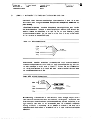
  • 1. Forouzan: Data I II. Physical layer and I 6. Bandwidth Utilization: I I © The McGraw-Hill I Communications and Media Multiplexing and Companies, 2007 Networking, Fourth Edition Spreading 174 CHAPTER 6 BANDWIDTH UTILIZATION: MULTIPLEXING AND SPREADING if data rates are not the same, three strategies, or a combination of them, can be used. We call these three strategies multilevel multiplexing, multiple-slot allocation, and pulse stuffing. Multilevel Multiplexing Multilevel multiplexing is a technique used when the data rate of an input line is a multiple of others. For example, in Figure 6.19, we have two inputs of 20 kbps and three inputs of 40 kbps. The first two input lines can be multi- plexed together to provide a data rate equal to the last three. A second level of multi- plexing can create an output of 160 kbps. Figure 6.19 Multilevel multiplexing 20 kbps 20 kbps 40 kbps 40 kbps 40 kbps 0 kbps 0 kbps V 160 kbps Multiple-Slot Allocation Sometimes it is more efficient to allot more than one slot in a frame to a single input line. For example, we might have an input line that has a data rate that is a multiple of another input. In Figure 6.20, the input line with a 50-kbps data rate can be given two slots in the output. We insert a serial-to-parallel converter in the line to make two inputs out of one. Figure 6.20 Multiple-slot multiplexing 25 kbps 50 kbps • 25 kbps 25 kbps • 25 kbps • 25 kbps The input with a 50-kHz data rate has two slots in each frame. • 125 kbps Pulse Stuffing Sometimes the bit rates of sources are not multiple integers of each other. Therefore, neither of the above two techniques can be applied. One solution is to make the highest input data rate the dominant data rate and then add dummy bits to the input lines with lower rates. This will increase their rates. This technique is called pulse stuffing, bit padding, or bit stuffing. The idea is shown in Figure 6.21. The input with a data rate of 46 is pulse-stuffed to increase the rate to 50 kbps. Now multiplexing can take place.
  • 2. II. Physical Layer and Media 6. Bandwidth Utilization: Multiplexing and Spreading SECTION 6.1 MULTIPLEXING 175 Figure 6.21 Pulse stuffing 50 kbps 50 kbps 46 kbps Frame Synchronizing The implementation of TDM is not as simple as that of FDM. Synchronization between the multiplexer and demultiplexer is a major issue. If the multiplexer and the demulti- plexer are not synchronized, a bit belonging to one channel may be received by the wrong channel. For this reason, one or more synchronization bits are usually added to the beginning of each frame. These bits, called framing bits, follow a pattern, frame to frame, that allows the demultiplexer to synchronize with the incoming stream so that it can separate the time slots accurately. In most cases, this synchronization information consists of 1 bit per frame, alternating between 0 and 1, as shown in Figure 6.22. Figure 6.22 Framing bits 1 o 1 I Synchronization pattern Frame 3 C3 ! B3 ! A3 Frame 2 1 B2 ! A2 • Frame 1 ! CI | i | Al ! B' in Example 6.10 We have four sources, each creating 250 characters per second. If the interleaved unit is a character and 1 synchronizing bit is added to each frame, find (a) the data rate of each source, (b) the duration of each character in each source, (c) the frame rate, (d) the duration of each frame, (e) the number of bits in each frame, and (f) the data rate of the link. Solution We can answer the questions as follows: a. The data rate of each source is 250 x 8 = 2000 bps = 2 kbps. b. Each source sends 250 characters per second; therefore, the duration of a character is 1/250 s, or 4 ms. c. Each frame has one character from each source, which means the link needs to send 250 frames per second to keep the transmission rate of each source. d. The duration of each frame is 1/250 s, or 4 ms. Note that the duration of each frame is the same as the duration of each character coming from each source. e. Each frame carries 4 characters and 1 extra synchronizing bit. This means that each frame is 4 x 8 + 1 = 33 bits.
  • 3. Forouzan: Data I II. Physical Layer and I 6. Bandwidth Utilization: I I © The McGraw-Hill I Communications and Media Multiplexing and Companies, 2007 Networking, Fourth Edition Spreading 176 CHAPTER 6 BANDWIDTH UTILIZATION: MULTIPLEXING AND SPREADING f. The link sends 250 frames per second, and each frame contains 33 bits. This means that the data rate of the link is 250 x 33, or 8250 bps. Note that the bit rate of the link is greater than the combined bit rates of the four channels. If we add the bit rates of four channels, we get 8000 bps. Because 250 frames are traveling per second and each contains 1 extra bit for synchronizing, we need to add 250 to the sum to get 8250 bps. Example 6.11 Two channels, one with a bit rate of 100 kbps and another with a bit rate of 200 kbps, are to be multiplexed. How this can be achieved? What is the frame rate? What is the frame duration? What is the bit rate of the link? Solution We can allocate one slot to thefirstchannel and two slots to the second channel. Each frame car- ries 3 bits. The frame rate is 100,000 frames per second because it carries 1 bit from the first channel. The frame duration is 1/100,000 s, or 10 ms. The bit rate is 100,000 frames/s x 3 bits per frame, or 300 kbps. Note that because each frame carries 1 bit from thefirstchannel, the bit rate for the first channel is preserved. The bit rate for the second channel is also preserved because each frame carries 2 bits from the second channel. Digital Signal Service Telephone companies implement TDM through a hierarchy of digital signals, called digital signal (DS) service or digital hierarchy. Figure 6.23 shows the data rates sup- ported by each level. Figure 6.23 Digital hierarchy • A DS-0 service is a single digital channel of 64 kbps. • DS-1 is a 1.544-Mbps service; 1.544 Mbps is 24 times 64 kbps plus 8 kbps of overhead. It can be used as a single service for 1.544-Mbps transmissions, or it can be used to multiplex 24 DS-0 channels or to carry any other combination desired by the user that can fit within its 1.544-Mbps capacity. • DS-2 is a 6.312-Mbps service; 6.312 Mbps is 96 times 64 kbps plus 168 kbps of overhead. It can be used as a single service for 6.312-Mbps transmissions; or it can
  • 4. Forouzan: Data Communications and Networking, Fourth Edition II. Physical Layer and Media 6. Bandwidth Utilization: Multiplexing and Spreading ©The McGraw-Hill Companies, 2007 SECTION 6.1 MULTIPLEXING 177 be used to multiplex 4 DS-1 channels, 96 DS-0 channels, or a combination of these service types. • DS-3 is a 44.376-Mbps service; 44.376 Mbps is 672 times 64 kbps plus 1.368 Mbps of overhead. It can be used as a single service for 44.376-Mbps transmissions; or it can be used to multiplex 7 DS-2 channels, 28 DS-1 channels, 672 DS-0 channels, or a combination of these service types. • DS-4 is a 274.176-Mbps service; 274.176 is 4032 times 64 kbps plus 16.128 Mbps of overhead. It can be used to multiplex 6 DS-3 channels, 42 DS-2 channels, 168 DS-1 channels, 4032 DS-0 channels, or a combination of these service types. DS-0, DS-1, and so on are the names of services. To implement those services, the tele- phone companies use T lines (T-l to T-4). These are lines with capacities precisely matched to the data rates of the DS-1 to DS-4 services (see Table 6.1). So far only T-l and T-3 lines are commercially available. Table 6.1 DS and T line rates Service Line Rate (Mbps) Voice Channels DS-1 T-l 1.544 24 DS-2 T-2 6.312 96 DS-3 T-3 44.736 672 DS-4 T-4 274.176 4032 The T-l line is used to implement DS-1; T-2 is used to implement DS-2; and so on. As you can see from Table 6.1, DS-0 is not actually offered as a service, but it has been defined as a basis for reference purposes. T Lines for Analog Transmission T lines are digital lines designed for the transmission of digital data, audio, or video. However, they also can be used for analog transmission (regular telephone connec- tions), provided the analog signals are first sampled, then time-division multiplexed. The possibility of using T lines as analog carriers opened up a new generation of services for the telephone companies. Earlier, when an organization wanted 24 separate telephone lines, it needed to run 24 twisted-pair cables from the company to the central exchange. (Remember those old movies showing a busy executive with 10 telephones lined up on his desk? Or the old office telephones with a big fat cable running from them? Those cables contained a bundle of separate lines.) Today, that same organization can combine the 24 lines into one T-l line and run only the T-l line to the exchange. Figure 6.24 shows how 24 voice channels can be multiplexed onto one T-l line. (Refer to Chapter 5 for PCM encoding.) The T-l Frame As noted above, DS-1 requires 8 kbps of overhead. To understand how this overhead is calculated, we must examine the format of a 24-voice-channel frame. The frame used on a T-l line is usually 193 bits divided into 24 slots of 8 bits each plus 1 extra bit for synchronization (24 x 8 + 1 = 193); see Figure 6.25. In other words, T Lines
  • 5. Forouzan: Data I II. Physical Layer and I 6. Bandwidth Utilization: I I © The McGraw-Hill Communications and Media Multiplexing and Companies, 2007 Networking, Fourth Edition Spreading 178 CHAPTER 6 BANDWIDTH UTILIZATION: MULTIPLEXING AND SPREADING Figure 6.24 T-l linefor multiplexing telephone lines /Sampling at 8000 samples/sN V using 8 bits per sample J T-l line 1.544 Mbps 24 x 64 kbps + 8 kbps overhead each slot contains one signal segment from each channel; 24 segments are interleaved in one frame. If a T-l line carries 8000 frames, the data rate is 1.544 Mbps (193 x 8000 = 1.544 Mbps)—the capacity of the line. E Lines Europeans use a version of T lines called E lines. The two systems are conceptually iden- tical, but their capacities differ. Table 6.2 shows the E lines and their capacities.
  • 6. Forouzan: Data I II. Physical Layer and I 6. Bandwidth Utilization: I I © The McGraw-Hill Communications and Media Multiplexing and Companies, 2007 Networking, Fourth Edition Spreading SECTION 6.1 MULTIPLEXING 179 Table 6.2 E line rates Line Rate (Mbps) Voice Channels E-1 2.048 30 E-2 8.448 120 E-3 34.368 480 E-4 139.264 1920 More Synchronous TDM Applications Some second-generation cellular telephone companies use synchronous TDM. For example, the digital version of cellular telephony divides the available bandwidth into 30-kHz bands. For each band, TDM is applied so that six users can share the band. This means that each 30-kHz band is now made of six time slots, and the digitized voice sig- nals of the users are inserted in the slots. Using TDM, the number of telephone users in each area is now 6 times greater. We discuss second-generation cellular telephony in Chapter 16. Statistical Time-Division Multiplexing As we saw in the previous section, in synchronous TDM, each input has a reserved slot in the output frame. This can be inefficient if some input lines have no data to send. In statistical time-division multiplexing, slots are dynamically allocated to improve band- width efficiency. Only when an input line has a slot's worth of data to send is it given a slot in the output frame. In statistical multiplexing, the number of slots in each frame is less than the number of input lines. The multiplexer checks each input line in round- robin fashion; it allocates a slot for an input line if the line has data to send; otherwise, it skips the line and checks the next Line. Figure 6.26 shows a synchronous and a statistical TDM example. In the former, some slots are empty because the corresponding line does not have data to send. In the latter, however, no slot is left empty as long as there are data to be sent by any input line. Addressing Figure 6.26 also shows a major difference between slots in synchronous TDM and statistical TDM. An output slot in synchronous TDM is totally occupied by data; in statistical TDM, a slot needs to carry data as well as the address of the destination. In synchronous TDM, there is no need for addressing; synchronization and preassigned relationships between the inputs and outputs serve as an address. We know, for exam- ple, that input 1 always goes to input 2. If the multiplexer and the demultiplexer are synchronized, this is guaranteed. In statistical multiplexing, there is no fixed relation- ship between the inputs and outputs because there are no preassigned or reserved slots. We need to include the address of the receiver inside each slot to show where it is to be delivered. The addressing in its simplest form can be n bits to define N different output lines with n = log2 N. For example, for eight different output lines, we need a 3-bit address.
  • 7. Forouzan: Data I II. Physical Layer and I 6. Bandwidth Utilization: I I © The McGraw-Hill I Communications and Media Multiplexing and Companies, 2007 Networking, Fourth Edition Spreading 180 CHAPTER 6 BANDWIDTH UTILIZATION: MULTIPLEXING AND SPREADING Figure 6.26 TDM slot comparison a. Synchronous TDM Line A 1 A1 r LineB—I H2 H~~Bl [ Line C Line D —I P2 Line E b. Statistical TDM Slot Size Since a slot carries both data and an address in statistical TDM, the ratio of the data size to address size must be reasonable to make transmission efficient. For example, it would be inefficient to send 1 bit per slot as data when the address is 3 bits. This would mean an overhead of 300 percent. In statistical TDM, a block of data is usually many bytes while the address is just a few bytes. No Synchronization Bit There is another difference between synchronous and statistical TDM, but this time it is at the frame level. The frames in statistical TDM need not be synchronized, so we do not need synchronization bits. Bandwidth In statistical TDM, the capacity of the link is normally less than the sum of the capaci- ties of each channel. The designers of statistical TDM define the capacity of the link based on the statistics of the load for each channel. If on average only x percent of the input slots are filled, the capacity of the link reflects this. Of course, during peak times, some slots need to wait. 6.2 SPREAD SPECTRUM Multiplexing combines signals from several sources to achieve bandwidth efficiency; the available bandwidth of a link is divided between the sources. In spread spectrum (SS), we also combine signals from different sources to fit into a larger bandwidth, but our goals
  • 8. 6. Bandwidth Utilization: Multiplexing and Spreading SECTION 6.2 SPREAD SPECTRUM 181 are somewhat different. Spread spectrum is designed to be used in wireless applications (LANs and WANs). In these types of applications, we have some concerns that outweigh bandwidth efficiency. In wireless applications, all stations use air (or a vacuum) as the medium for communication. Stations must be able to share this medium without intercep- tion by an eavesdropper and without being subject to jamming from a malicious intruder (in military operations, for example). To achieve these goals, spread spectrum techniques add redundancy; they spread the original spectrum needed for each station. If the required bandwidth for each station is B, spread spectrum expands it to B s s , such that B s s » B. The expanded bandwidth allows the source to wrap its message in a protective envelope for a more secure trans- mission. An analogy is the sending of a delicate, expensive gift. We can insert the gift in a special box to prevent it from being damaged during transportation, and we can use a superior delivery service to guarantee the safety of the package. Figure 6.27 shows the idea of spread spectrum. Spread spectrum achieves its goals through two principles: 1. The bandwidth allocated to each station needs to be, by far, larger than what is needed. This allows redundancy. 2. The expanding of the original bandwidth B to the bandwidth Bss must be done by a process that is independent of the original signal. In other words, the spreading process occurs after the signal is created by the source. Figure 6.27 Spread spectrum Spreading Spreading process I Spreading code After the signal is created by the source, the spreading process uses a spreading code and spreads the bandwidth. The figure shows the original bandwidth B and the spreaded bandwidth Bss. The spreading code is a series of numbers that look random, but are actually a pattern. There are two techniques to spread the bandwidth: frequency hopping spread spec- trum (FHSS) and direct sequence spread spectrum (DSSS). Frequency Hopping Spread Spectrum (FHSS) The frequency hopping spread spectrum (FHSS) technique uses M different carrier frequencies that are modulated by the source signal. At one moment, the signal modu- lates one carrier frequency; at the next moment, the signal modulates another carrier
  • 9. Forouzan: Data I II. Physical Layer and I 6. Bandwidth Utilization: I I © The McGraw-Hill I ^ Communications and Media Multiplexing and Companies, 2007 Networking, Fourth Edition Spreading 182 CHAPTER 6 BANDWIDTH UTILIZATION: MULTIPLEXING AND SPREADING frequency. Although the modulation is done using one carrier frequency at a time, M frequencies are used in the long run. The bandwidth occupied by a source after spreading is fipnss > : > Figure 6.28 shows the general layout for FHSS. A pseudorandom code generator, called pseudorandom noise (PN), creates afc-bitpattern for every hopping period T^. The frequency table uses the pattern to find the frequency to be used for this hopping period and passes it to the frequency synthesizer. The frequency synthesizer creates a carrier signal of that frequency, and the source signal modulates the carrier signal. Figure 6.28 Frequency hopping spread spectrum (FHSS) Original signal .2 3' Modulator _ Spread signal Frequency synthesizer Frequency table Suppose we have decided to have eight hopping frequencies. This is extremely low for real applications and is just for illustration. In this case, M is 8 and k is 3. The pseudo- random code generator will create eight different 3-bit patterns. These are mapped to eight different frequencies in the frequency table (see Figure 6.29). Figure 6.29 Frequency selection in FHSS First-hop frequency fe-bit patterns ioi in ooi ooo oio no on 100 First selection it-bit 000 001 010 on 100 -101 110 111 Frequency 200 kH? 300 kHz 400 kHz 500 kHz 600 kHz 700 kHz - 800 kHz 900 kHz Frequency table
  • 10. Forouzan: Data I II. Physical Layer and I 6. Bandwidth Utilization: I I © The McGraw-Hill Communications and Media Multiplexing and Companies, 2007 Networking, Fourth Edition Spreading SECTION 6.2 SPREAD SPECTRUM 183 The pattern for this station is 101, 111, 001, 000, 010, 011, 100. Note that the pat- tern is pseudorandom it is repeated after eight hoppings. This means that at hopping period 1, the pattern is 101. The frequency selected is 700 kHz; the source signal mod- ulates this carrier frequency. The secondfc-bitpattern selected is 111, which selects the 900-kHz carrier; the eighth pattern is 100, the frequency is 600 kHz. After eight hop- pings, the pattern repeats, starting from 101 again. Figure 6.30 shows how the signal hops around from carrier to carrier. We assume the required bandwidth of the original signal is 100 kHz. Figure 6.30 FHSS cycles Carrier frequencies (kHz) 900 800 700 600 500 400 300 200 Cycle 1 ~A IBB • M M * ; - Q - Cycle 2 • • 1 2 3 4 5 6 7 8 9 10 11 12 13 14 15 16 Hop periods It can be shown that this scheme can accomplish the previously mentioned goals. If there are many fc-bit patterns and the hopping period is short, a sender and receiver can have privacy. If an intruder tries to intercept the transmitted signal, she can only access a small piece of data because she does not know the spreading sequence to quickly adapt herself to the next hop. The scheme has also an antijamming effect. A malicious sender may be able to send noise to jam the signal for one hopping period (randomly), but not for the whole period. Bandwidth Sharing If the number of hopping frequencies is M, we can multiplex M channels into one by using the same B s s bandwidth. This is possible because a station uses just one frequency in each hopping period; M - 1 other frequencies can be used by other M - 1 stations. In other words, M different stations can use the same Bss if an appropriate modulation technique such as multiple FSK (MFSK) is used. FHSS is similar to FDM, as shown in Figure 6.31. Figure 6.31 shows an example of four channels using F D M and four channels using FHSS. In FDM, each station uses 1/M of the bandwidth, but the allocation is fixed; in FHSS, each station uses 1/M of the bandwidth, but the allocation changes hop to hop.
  • 11. Forouzan: Data I II. Physical Layer and I 6. Bandwidth Utilization: I I © The McGraw-Hill I Communications and Media Multiplexing and Companies, 2007 Networking, Fourth Edition Spreading 184 CHAPTER 6 BANDWIDTH UTILIZATION: MULTIPLEXING AND SPREADING Figure 6.31 Bandwidth sharing Direct Sequence Spread Spectrum The direct sequence spread spectrum (DSSS) technique also expands the bandwidth of the original signal, but the process is different. In DSSS, we replace each data bit with n bits using a spreading code. In other words, each bit is assigned a code of n bits, called chips, where the chip rate is n times that of the data bit. Figure 6.32 shows the concept of DSSS. Figure 6.32 DSSS Original signal Modulator Spread signal Chips generator As an example, let us consider the sequence used in a wireless LAN, the famous Barker sequence where n is 11. We assume that the original signal and the chips in the chip generator use polar NRZ encoding. Figure 6.33 shows the chips and the result of multiplying the original data by the chips to get the spread signal. In Figure 6.33, the spreading code is 11 chips having the pattern 10110111000 (in this case). If the original signal rate is N, the rate of the spread signal is 1 IN. This means that the required bandwidth for the spread signal is 11 times larger than the bandwidth of the original signal. The spread signal can provide privacy if the intruder does not know the code. It can also provide immunity against interference if each sta- tion uses a different code.
  • 12. 6. Bandwidth Utilization: Multiplexing and Spreading SECTION 6.4 KEY TERMS 185 Figure 6.33 DSSS example Original signal Spreading code Spread signal • 1 1 0 1 1 0 1 1 I " 1 1 — 1 1 0 0 0 j a i i o i i i 1 P I 1 U » 0 1 0 1 1 0 1 1 1 11—11 0 0 0] 1 u u "1 I — 1 1 u • n n u u II II 1 1 1 1 U J II '11', U Li 1 1 Bandwidth Sharing Can we share a bandwidth in DSSS as we did in FHSS? The answer is no and yes. If we use a spreading code that spreads signals (from different stations) that cannot be combined and separated, we cannot share a bandwidth. For example, as we will see in Chapter 14, some wireless LANs use DSSS and the spread bandwidth cannot be shared. However, if we use a special type of sequence code that allows the combining and separating of spread signals, we can share the bandwidth. As we will see in Chapter 16, a special spreading code allows us to use DSSS in cellular telephony and share a bandwidth between several users. 6.3 RECOMMENDED READING For more details about subjects discussed in this chapter, we recommend the following books. The items in brackets [...] refer to the reference list at the end of the text. Books Multiplexing is elegantly discussed in Chapters 19 of [Pea92]. [CouOl] gives excellent coverage of TDM and FDM in Sections 3.9 to 3.11. More advanced materials can be found in [Ber96]. Multiplexing is discussed in Chapter 8 of [Sta04]. A good coverage of spread spectrum can be found in Section 5.13 of [CouOl] and Chapter 9 of [Sta04]. 6.4 KEY TERMS analog hierarchy digital signal (DS) service Barker sequence direct sequence spread spectrum (DSSS) channel E line chip framing bit demultiplexer (DEMUX) frequency hopping spread spectrum dense WDM (DWDM) (FSSS)
  • 13. Forouzan: Data Communications and Networking, Fourth Edition II. Physical Layer and Media 6. Bandwidth Utilization: Multiplexing and Spreading ©The McGraw-Hill Companies, 2007 186 CHAPTER 6 BANDWIDTH UTILIZATION: MULTIPLEXING AND SPREADING • Bandwidth utilization is the use of available bandwidth to achieve specific goals. Efficiency can be achieved by using multiplexing; privacy and antijamming can be achieved by using spreading. • Multiplexing is the set of techniques that allows the simultaneous transmission of multiple signals across a single data link. In a multiplexed system, n lines share the bandwidth of one link. The word link refers to the physical path. The word channel refers to the portion of a link that carries a transmission. • There are three basic multiplexing techniques: frequency-division multiplexing, wavelength-division multiplexing, and time-division multiplexing. The first two are techniques designed for analog signals, the third, for digital signals • Frequency-division multiplexing (FDM) is an analog technique that can be applied when the bandwidth of a link (in hertz) is greater than the combined bandwidths of the signals to be transmitted. • Wavelength-division multiplexing (WDM) is designed to use the high bandwidth capability of fiber-optic cable. WDM is an analog multiplexing technique to com- bine optical signals. • Time-division multiplexing (TDM) is a digital process that allows several connec- tions to share the high bandwidth of a link. TDM is a digital multiplexing technique for combining several low-rate channels into one high-rate one. LI We can divide TDM into two different schemes: synchronous or statistical. In syn- chronous TDM, each input connection has an allotment in the output even if it is not sending data. In statistical TDM, slots are dynamically allocated to improve bandwidth efficiency. • In spread spectrum (SS), we combine signals from different sources to fit into a larger bandwidth. Spread spectrum is designed to be used in wireless applications in which stations must be able to share the medium without interception by an eavesdropper and without being subject to jamming from a malicious intruder. • The frequency hopping spread spectrum (FHSS) technique uses M different carrier frequencies that are modulated by the source signal. At one moment, the signal frequency-division multiplexing (FDM) group guard band hopping period interleaving jumbo group link master group multilevel multiplexing multiple-slot multiplexing multiplexer (MUX) multiplexing pseudorandom code generator pseudorandom noise (PN) pulse stuffing spread spectrum (SS) statistical TDM supergroup synchronous TDM T line time-division multiplexing (TDM) wavelength-division multiplexing (WDM) 6.5 SUMMARY
  • 14. Forouzan: Data Communications and Networking, Fourth Edition II. Physical Layer and Media 6. Bandwidth Utilization: Multiplexing and Spreading ©The McGraw-Hill Ccmpanies, 2007 SECTION 6.6 PRACTICE SET 187 modulates one carrier frequency; at the next moment, the signal modulates another carrier frequency. • The direct sequence spread spectrum (DSSS) technique expands the bandwidth of a signal by replacing each data bit with n bits using a spreading code. In other words, each bit is assigned a code of n bits, called chips. Review Questions 1. Describe the goals of multiplexing. 2. List three main multiplexing techniques mentioned in this chapter. 3. Distinguish between a link and a channel in multiplexing. 4. Which of the three multiplexing techniques is (are) used to combine analog signals? Which of the three multiplexing techniques is (are) used to combine digital signals? 5. Define the analog hierarchy used by telephone companies and list different levels of the hierarchy. 6. Define the digital hierarchy used by telephone companies and list different levels of the hierarchy. 7. Which of the three multiplexing techniques is common for fiber optic links? Explain the reason. 8. Distinguish between multilevel TDM, multiple slot TDM, and pulse-stuffed TDM. 9. Distinguish between synchronous and statistical TDM. 10. Define spread spectrum and its goal. List the two spread spectrum techniques dis- cussed in this chapter. 11. Define FHSS and explain how it achieves bandwidth spreading. 12. Define DSSS and explain how it achieves bandwidth spreading. Exercises 13. Assume that a voice channel occupies a bandwidth of 4 kHz. We need to multiplex 10 voice channels with guard bands of 500 Hz using FDM. Calculate the required bandwidth. 14. We need to transmit 100 digitized voice channels using a pass-band channel of 20 KHz. What should be the ratio of bits/Hz if we use no guard band? 15. In the analog hierarchy of Figure 6.9, find the overhead (extra bandwidth for guard band or control) in each hierarchy level (group, supergroup, master group, and jumbo group). 16. We need to use synchronous TDM and combine 20 digital sources, each of 100 Kbps. Each output slot carries 1 bit from each digital source, but one extra bit is added to each frame for synchronization. Answer the following questions: a. What is the size of an output frame in bits? b. What is the output frame rate? 6.6 PRACTICE SET
  • 15. Forouzan: Data Communications and Networking, Fourth Edition II. Physical Layer and Media 6. Bandwidth Utilization: Multiplexing and Spreading ©The McGraw-Hill Companies, 2007 188 CHAPTER 6 BANDWIDTH UTILIZATION: MULTIPLEXING AND SPREADING c. What is the duration of an output frame? d. What is the output data rate? e. What is the efficiency of the system (ratio of useful bits to the total bits). 17. Repeat Exercise 16 if each output slot carries 2 bits from each source. 1.8. We have 14 sources, each creating 500 8-bit characters per second. Since only some of these sources are active at any moment, we use statistical TDM to combine these sources using character interleaving. Each frame carries 6 slots at a time, but we need to add four-bit addresses to each slot. Answer the following questions: a. What is the size of an output frame in bits? b. What is the output frame rate? c. What is the duration of an output frame? d. What is the output data rate? 19. Ten sources, six with a bit rate of 200 kbps and four with a bit rate of 400 kbps are to be combined using multilevel TDM with no synchronizing bits. Answer the fol- lowing questions about the final stage of the multiplexing: a. What is the size of a frame in bits? b. What is the frame rate? c. What is the duration of a frame? d. What is the data rate? 20. Four channels, two with a bit rate of 200 kbps and two with a bit rate of 150 kbps, are to be multiplexed using multiple slot TDM with no synchronization bits. Answer the following questions: a. What is the size of a frame in bits? b. What is the frame rate? c. What is the duration of a frame? d. What is the data rate? 21. Two channels, one with a bit rate of 190 kbps and another with a bit rate of 180 kbps, are to be multiplexed using pulse stuffing TDM with no synchronization bits. Answer the following questions: a. What is the size of a frame in bits? b. What is the frame rate? c. What is the duration of a frame? d. What is the data rate? 22. Answer the following questions about a T-l line: a. What is the duration of a frame? b. What is the overhead (number of extra bits per second)? 23. Show the contents of the five output frames for a synchronous TDM multiplexer that combines four sources sending the following characters. Note that the characters are sent in the same order that they are typed. The third source is silent. a. Source 1 message: HELLO b. Source 2 message: HI
  • 16. 6. Bandwidth Utilization: Multiplexing and Spreading SECTION 6.6 PRACTICE SET 189 c. Source 3 message: d. Source 4 message: B Y E 24. Figure 6.34 shows a multiplexer in a synchronous TDM system. Each output slot is only 10 bits long (3 bits taken from each input plus 1 framing bit). What is the output stream? The bits arrive at the multiplexer as shown by the arrows. Figure 6.34 Exercise 24 101110111101 11111110000 1010000001111 Frame of 10 bits 25. Figure 6.35 shows a demultiplexer in a synchronous TDM. If the input slot is 16 bits long (no framing bits), what is the bit stream in each output? The bits arrive at the demultiplexer as shown by the arrows. Figure 6.35 Exercise 25 10100000 1010101010100001 0111000001111000 26. Answer the following questions about the digital hierarchy in Figure 6.23: a. What is the overhead (number of extra bits) in the DS-1 service? b. What is the overhead (number of extra bits) in the DS-2 service? c. What is the overhead (number of extra bits) in the DS-3 service? d. What is the overhead (number of extra bits) in the DS-4 service? 27. What is the minimum number of bits in a PN sequence if we use FHSS with a channel bandwidth of B = 4 KHz and B s s = 100 KHz? 28. An FHSS system uses a 4-bit PN sequence. If the bit rate of the PN is 64 bits per second, answer the following questions: a. What is the total number of possible hops? b. What is the time needed to finish a complete cycle of PN?
  • 17. Forouzan: Data Communications and Networking, Fourth Edition II. Physical Layer and Media 6. Bandwidth Utilization: Multiplexing and Spreading © The McGraw-Hill Companies. 2007 190 CHAPTER 6 BANDWIDTH UTILIZATION: MULTIPLEXING AND SPREADING 29. A pseudorandom number generator uses the following formula to create a random series: In which Ns defines the current random number and N i + 1 defines the next random number. The term mod means the value of the remainder when dividing (5 + 7Nj) by 17. 30. We have a digital medium with a data rate of 10 Mbps. How many 64-kbps voice channels can be carried by this medium if we use DSSS with the Barker sequence? N w =(5 + 7Nj)mod 17-1
  • 18. Forouzan: Data Communications and II. Physical Layer and Media 7. Transmission Media © The McGraw-Hill Companies, 2007 Transmission Media We discussed many issues related to the physical layer in/Thapters 3 through 6. In this chapter, discuss transmission media. Transmission media are actually located below the physicaKlayer and are directly controlled by the physical layer. You could say that transmission media belong to layer zero. Figure l.l/hows the position of transmission media in relation to the physical layer. Figure 7.1 Transmissiorhnedium andphysical lAyer Sender Physical layer Physical layer Receiver Trai fission medium Cable* A transmission medium c/n be broadly denied as anything that can carry infor- mation from a source to a destination. For example>tfie transmission medium for two people having a dinner conversation is the air. The aincan also be used to convey the message in a smoke signayor semaphore. For a writterKmessage, the transmission medium might be a mail ramier, a truck, or an airplane. In data communications the definition of the informationSmd the transmission medium is more specific/The transmission medium is usually free sp&re, metallic cable, or fiber-optic cable. The information is usually a signal that is the result Orva conversion of data from another /orm. The use of long-distance communication using electric signals started with the invention of the telegraph by Morse in the 19th century. Communication by telegraph was slow and dependent on a metallic medium. Extending the range of the human voice became possible when the telephone was invented in 1869. Telephone communication at that time also needed a metallic medium to carry the electric signals that were the result of a conversion from the human voice. 191