Linearization technique of nonlinear things

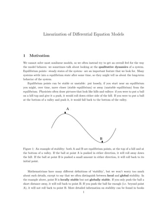
1. Linearization of Differential Equation Models
1 Motivation
We cannot solve most nonlinear models, so we often instead try to get an overall feel for the way
the model behaves: we sometimes talk about looking at the qualitative dynamics of a system.
Equilibrium points– steady states of the system– are an important feature that we look for. Many
systems settle into a equilibrium state after some time, so they might tell us about the long-term
behavior of the system.
Equilibrium points can be stable or unstable: put loosely, if you start near an equilibrium
you might, over time, move closer (stable equilibrium) or away (unstable equilibrium) from the
equilibrium. Physicists often draw pictures that look like hills and valleys: if you were to put a ball
on a hill top and give it a push, it would roll down either side of the hill. If you were to put a ball
at the bottom of a valley and push it, it would fall back to the bottom of the valley.
A
B
Figure 1: An example of stability: both A and B are equilibrium points, at the top of a hill and at
the bottom of a valley. If the ball at point A is pushed in either direction, it will roll away down
the hill. If the ball at point B is pushed a small amount in either direction, it will roll back to its
initial point.
Mathematicians have many different definitions of ‘stability’, but we won’t worry too much
about such details, except to say that we often distinguish between local and global stability. In
the example above, point B is locally stable but not globally stable. If you only push the ball a
short distance away, it will roll back to point B. If you push the ball far enough (i.e. beyond point
A), it will not roll back to point B. More detailed information on stability can be found in books
1

2. on nonlinear differential equations or dynamical systems (for instance S. H. Strogatz’s ‘Nonlinear
Dynamics and Chaos’).
Linearization can be used to give important information about how the system behaves in the
neighborhood of equilibrium points. Typically we learn whether the point is stable or unstable, as
well as something about how the system approaches (or moves away from) the equilibrium point.
The basic idea is that (in most circumstances) one can approximate the nonlinear differential
equations that govern the behavior of the system by linear differential equations. We can solve
the resulting set of linear ODEs, whereas we cannot, in general, solve a set of nonlinear differential
equations.
2 How to Linearize a Model
We shall illustrate the linearization process using the SIR model with births and deaths in a
population of fixed size.
Ṡ = µN − βSI/N − µS (1)
˙
I = βSI/N − (γ + µ)I (2)
Ṙ = γI − µR, (3)
with S + I + R = N. Since we assume that the population is closed, we can always calculate the
value of R if we know S and I. Therefore we need only focus on the first two equations for S and
I.
We denote an equilibrium point by attaching asterisks to the state variables: e.g. an equilibrium
point of the SIR model may be written as (S∗, I∗). Because an equilibrium point means that the
values of S and I (and R) remain constant, this means that dS/dt = dI/dt = 0 when (S, I) =
(S∗, I∗).
If we imagine that both S and I are close to the equilibrium point, then the differences S − S∗,
which we denote by x1, and I − I∗, which we denote by x2, will be small. An important point
is that terms involving products of x1 and x2 (e.g. the quadratic terms x2
1, x2
2 or x1x2) are much
smaller still and so, to a very good approximation, can be ignored.
We can differentiate our expression for x1: dx1/dt = dS/dt − dS∗/dt. Since S∗ is a constant,
we have dx1/dt = dS/dt and, using a similar argument, dx2/dt = dI/dt. So we now have
ẋ1 = µN − βSI/N − µS (4)
ẋ2 = βSI/N − (γ + µ)I. (5)
But these equations are in terms of the original variables, S and I.
There are two ways in which we can then obtain the linearization. One is a calculus-free method,
the other uses the idea of Taylor series from calculus.

3. 2.1 Non-calculus method:
We rewrite the previous equations in terms of x1 and x2 using S = S∗ + x1 and I = I∗ + x2.
ẋ1 = µN − β(S∗
+ x1)(I∗
+ x2)/N − µ(S∗
+ x1) (6)
ẋ2 = β(S∗
+ x1)(I∗
+ x2)/N − (γ + µ)(I∗
+ x2). (7)
If we multiply out the brackets that appear in the infection term, we have
βSI/N = (β/N)(S∗
+ x1)(I∗
+ x2) (8)
= (β/N)(S∗
I∗
+ S∗
x2 + I∗
x1 + x1x2 (9)
≈ (β/N)(S∗
I∗
+ S∗
x2 + I∗
x1). (10)
Where, to reach the last step we made use of the fact that we noted above: the product x1x2 is
very small indeed and so can be ignored.
This leads to the following:
ẋ1 = µN − βS∗
I∗
/N − µS∗
+ β(S∗
x2 + I∗
x1)/N − µx1 (11)
ẋ2 = βS∗
I∗
/N − (γ + µ)I∗
+ β(S∗
x2 + I∗
x1)/N − (γ + µ)x2. (12)
Since (S∗, I∗) is an equilibrium point, the original model equations tell us that µN − βS∗I∗/N −
µS∗ = 0 and βS∗I∗/N − (γ + µ)I∗ = 0. This allows us to cancel some terms in these equations and
we are left with the following linearized equations:
ẋ1 = (β/N)(S∗
x2 + I∗
x1) − µx1 (13)
ẋ2 = (β/N)(S∗
x2 + I∗
x1) − (γ + µ)x2. (14)
2.2 Calculus method:
By using a Taylor series expansion, we can arrive a little more quickly at the linearization.
As a shorthand, we write the right hand side of the dS/dt equation as f(S, I) (e.g. f(S, I) =
µN − βSI/N − µS) and the right hand side of the dI/dt equation as g(S, I). We then expand
about the point (S∗, I∗) to give
dS
dt
= f(S∗
, I∗
) + (S − S∗
)
∂f
∂S
+ (I − I∗
)
∂f
∂I
+ (higher order terms) (15)
dI
dt
= g(S∗
, I∗
) + (S − S∗
)
∂g
∂S
+ (I − I∗
)
∂g
∂I
+ (higher order terms). (16)
Here, both partial derivatives are evaluated at the point (S∗, I∗). (In case you aren’t familiar with
partial derivatives: when you work out ∂f/∂S, you imagine that I is a constant. For the SIR
model, ∂f/∂S = βI/N − µ and ∂f/∂I = βS/N.)
Since (S∗, I∗) is an equilibrium point, we have that f(S∗, I∗) equals zero, since dS/dt = 0 at this
point and g(S∗, I∗) = 0 since dI/dt = 0. Remembering that x1 = S − S∗ and x2 = I − I∗ and that

4. dx1/dt = dS/dt and dx2/dt = dI/dt we have
dx1
dt
= x1
∂f
∂S
+ x2
∂f
∂I
(17)
dx2
dt
= x1
∂g
∂S
+ x2
∂g
∂I
, (18)
where we have again ignored the higher order terms since they are of much smaller size.
For the SIR model, this becomes
ẋ1 = (βI∗
/N − µ)x1 − (βS∗
/N)x2 (19)
ẋ2 = (βI∗
/N)x1 + (βS∗
/N − γ − µ)x2. (20)
These are the same equations that we had before. Once you are familiar with the process, it’s very
easy to obtain the linearized equations in this way.
2.3 Matrix Notation for the Linearization
We can write linearizations in matrix form:
ẋ1
ẋ2
!
=
∂f
∂S
∂f
∂I
∂g
∂S
∂g
∂I
!
x1
x2
!
, (21)
or in shorthand
ẋ = Jx, (22)
where J is the so-called Jacobian matrix, whose entries are the partial derivatives of the right hand
sides of the differential equations describing the model, taken with respect to the different state
variables of the model (e.g. S and I). We often write the entries of J as
J =
a11 a12
a21 a22
!
. (23)
We can do this linearization process for a model with any number of state variables: if there are
n state variables, we get an n-dimensional set of coupled linear differential equations. (Bear in
mind that for the SIR model there are three state variables, S, I and R, but our assumption that
S + I + R = N leads to our only having to consider a two dimensional system.)
3 What do we do with the linearization?
There is a well-developed theory for solving linear differential equations such as (22). We can
only cover the briefest points here: for more information, find a book on differential equations or
an introductory mathematical biology text. (You might start with chapter 5 of S. H. Strogatz’s
‘Nonlinear Dynamics and Chaos’).

5. 3.1 One Dimensional Case
It’s perhaps simplest to start with the corresponding one-dimensional equation:
ẋ = λx. (24)
This equation has solution
x(t) = ceλt
, (25)
where c is the initial value of x (i.e. the value taken by x when t = 0). This equation describes
exponential growth or decay.
If λ is greater than zero, then points move away from x = 0. Remembering that x = 0
corresponds to the equilibrium point, we see that non-zero points move away from the equilibrium
as time passes: the equilibrium is unstable. If λ is less than zero, points move towards x = 0: the
equilibrium is unstable. If λ = 0, points neither move towards nor away from the equilibrium.
The sign of λ tells us about the stability of the equilibrium, and the size of λ tells us something
about how quickly points move away from or towards the equilibrium. When we have a stable
equilibrium, we sometimes talk about the relaxation time, which is defined to be −1/λ. This is
the time taken for the distance between the point and the origin to decrease by a factor 1/e ≈ 0.368.
We can summarize the behaviors in the following figures, in which arrows denote the directions
in which points move.
0 x 0 x
Figure 2: The left panel illustrates an unstable equilibrium, the right panel a stable equilibrium.
3.2 Two Dimensional Case
By analogy with the one dimensional case, we try a solution of the form
x1
x2
!
=
v1
v2
!
eλt
, (26)
where λ, v1 and v2 are constants. In shorthand notation we have
x(t) = veλt
. (27)
If we differentiate x(t) directly, we see that its derivative is given by
ẋ(t) = λveλt
. (28)
But we know that x(t) has to satisfy dx/dt = Jx, so we have
ẋ = J
veλt
. (29)
= (Jv) eλt
. (30)

6. Comparing (28) and (29) we see that v and λ must satisfy
Jv = λv. (31)
In linear algebra, such vectors v are known as eigenvectors of the matrix J and the constants λ
are known as eigenvalues of the matrix. Because these are important properties of matrices, there
is quite a large theory devoted to calculating their values. (If you need to know more, a good place
to start looking is a linear algebra textbook.) In the two dimensional case, the matrix J typically
has two independent eigenvectors and two eigenvalues (although the two eigenvalues can be equal).
Because we have a two dimensional set of linear differential equations, the general solution is, in
most cases 1, given by the sum of two terms of the form (27): x(t) = c1v1eλ1t +c2v2eλ2t. (The fact
that one can add solutions together in this way is a fundamental property of linear systems, and
one which makes them nice to work with.) The constants c1 and c2 are determined by the initial
conditions. Notice that this form of the solution shows that the eigenvectors define two directions
along which there may be exponential growth or decay. We will see this in action later on.
3.2.1 Finding the Eigenvalues and Eigenvectors in the 2D Case
We now need to find the eigenvalues and eigenvectors. Rearranging (31) gives us
(J − λI)v = 0, (32)
where I is the two dimensional identity matrix
I =
1 0
0 1
!
. (33)
Theory from linear algebra shows that such an equation can only have a non-trivial solution (i.e.
one in which v is not equal to zero) if the determinant of the matrix J − λI is equal to zero.
For a 2×2 matrix with entries aij (e.g. as in equation (23)), the determinant of the matrix is given
by the product of the two entries on the leading diagonal minus the product of the two entries on
the other diagonal: a11a22 − a12a21.
Using this definition, we see that in order for λ to be an eigenvalue of the matrix J, it must satisfy
(a11 − λ) (a22 − λ) − a12a21 = 0. (34)
(Notice that the ‘−λ’ terms arise because we have J − λI, and the matrix I has entries equal to
one in the (1,1) and (2,2) positions.)
Equation (34) is a quadratic equation for λ: notice that this gives us (in most cases) two possible
answers, λ1 and λ2. If we had an n-dimensional system, we would get a polynomial of degree n.
When n is anything other than a small number, such equations become difficult (or impossible) to
solve. But in the 2D case we can get an explicit expression for the eigenvalues. At worst, we can
always use the ‘quadratic formula’, but we can do a little better than this.
1
The general solution can be more complex if the matrix J does not have a complete set of linearly independent
eigenvectors. In such cases, the general solution has terms of the form p(t)veλt
, where p(t) is a polynomial in t.

7. Multiplying out (34) gives
λ2
− (a11 + a22) λ + (a11a22 − a12a21) = 0. (35)
We see that the linear term involves a11 + a22, the sum of the entries on the leading diagonal of J.
This sum is called the trace of the matrix J, tr J. The constant term of this quadratic is just the
determinant of the matrix J, det J. So we can rewrite (35) succinctly as
λ2
− tr Jλ + det J = 0. (36)
Since we know that the numbers λ1 and λ2 satisfy the quadratic equation for λ, we know that we
can factor this quadratic in the following way
(λ − λ1) (λ − λ2) = 0. (37)
Multiplying out this equation, we get
λ2
− (λ1 + λ2) λ + λ1λ2 = 0. (38)
Comparing (36) and (38) shows that
λ1 + λ2 = tr J (39)
λ1λ2 = det J. (40)
We can immediately write down the sum of the eigenvalues and their product in terms of the trace
and determinant of J: quantities that we can easily work out from the entries of J.
The formula for the solution of a quadratic equation, applied to (36) gives
λ = −
1
2
tr J ±
1
2
q
(tr J)2
− 4 det J . (41)
Notice that an important difference between the 1D and 2D cases is that we can now have complex
eigenvalues. This happens if the term inside the square root is negative, i.e. if (tr J)2
4 det J.
If we have a complex eigenvalue, which we can write in terms of its real and imaginary parts as
λ1 = ρ + iω, then it is fairly straightforward to show that λ2 = ρ − iω is also an eigenvalue. These
eigenvalues have equal real parts but their imaginary parts have opposite signs: this is called a
complex conjugate pair. There is a standard result that says if you have a polynomial whose
coefficients are real, then complex eigenvalues always come in such complex conjugate pairs. (Notice
that this result applies to our situation: the entries of the Jacobian matrix are real numbers.)
Notice that in the complex eigenvalue case, exp (λt) is of the form exp {(ρ ± iω)t}, which can be
multiplied out to give exp(ρt) exp(±iωt). The magnitude of exp(λt) is given by the term exp(ρt):
the real part of the eigenvalue, ρ, describes whether one has growth or decay. In the decay case,
the relaxation time is equal to −1/ρ. Since one can write
exp(iωt) = cos(ωt) + i sin(ωt), (42)
we see that the term exp(iωt) describes oscillatory behavior with constant amplitude, with (angular)
frequency ω. The period of the oscillation is given by 2π/ω.

8. 3.3 Complete Characterization of Behavior in 2D Case
We now make use of the above analysis of the eigenvalues in 2D to characterize all possible cases.
We make use of the fact that det J = λ1λ2 and tr J = λ1 + λ2 to find the signs of the eigenvalues
(or of their real parts in the complex case), as it is these quantities that determine stability. We
will leave discussion of so-called ‘borderline’ cases until the end: these borderline cases involve ones
in which either both eigenvalues are equal or one (or more) eigenvalues are equal (or have real part
equal) to zero.
• Both eigenvalues are real: (tr J)2
4 det J
• tr J 0
This means that the sum of the eigenvalues is positive.
There are two possible cases:
• det J 0
The product of the eigenvalues is also positive. This means that both λ1 and λ2
must be positive. In terms of the differential equation, we have exponential growth
in the directions represented by both v1 and v2. We call this situation an unstable
node. If we order the eigenvalues so that λ1 λ2 0, then we see that the
growth is faster in the direction defined by v1 and so trajectories starting close to
the equilibrium point tend to move away from the equilibrium in this direction.
• det J 0
The product of the eigenvalues is negative. This means that we must have one
positive (call it λ1) and one negative (λ2) eigenvalue. We have exponential growth
in the direction represented by λ1 but exponential decay in the direction represented
by λ2. This is called a saddle: points move towards the equilibrium in one direction,
but away from the equilibrium in the other.
0
0
v1
v2
0
0
v1
v2
Figure 3: Left panel illustrates a stable node, with λ1 λ2 0. Notice that trajectories leave the
equilibrium in the direction of v1. Right panel illustrates a saddle, with λ1 0 λ2. Notice that
trajectories approach the equilibrium in the direction of v2, but leave in the direction of v2.

9. • tr J 0
This means that the sum of the eigenvalues is negative.
There are two possible cases:
• det J 0
The product of the eigenvalues is positive. This means that both λ1 and λ2 must
be negative. In terms of the differential equation, we have exponential decay in the
directions represented by both v1 and v2. We call this situation a stable node.
If we order the eigenvalues so that λ1 λ2 (i.e. λ2 is more negative), we see that
the contraction in the v2 direction occurs more quickly than in the v1 direction.
This means that trajectories approach the equilibrium along the line defined by the
vector v1.
• det J 0
The product of the eigenvalues is negative. This means that we must have one
positive (call it λ1) and one negative (λ2) eigenvalue. As in the situation above, this
corresponds to a saddle.
0
0
v1
v2
0
0
v1
v2
Figure 4: Left panel illustrates a stable node, with 0 λ1 λ2. Notice that trajectories approach
the equilibrium in the direction of v1. Right panel illustrates a saddle.
• Eigenvalues are Complex: (tr J)2
4 det J
In this case tr J equals the sum of the real parts of the two eigenvalues. But we know that
these eigenvalues occur as a complex conjugate pair and so have equal real parts. The trace
of J tells us whether the real parts of the eigenvalues are positive or negative.
• tr J 0
The eigenvalues have positive real part, so we have exponential growth. Points move
away from the equilibrium point, but do so in an oscillatory manner as discussed above.
We call this an unstable spiral. Notice that the spiral may be elliptical in nature.

10. • tr J 0
The eigenvalues have negative real part, so we have exponential decay. Points move
towards the equilibrium point, but do so in an oscillatory manner as discussed above.
We call this a stable spiral.
0
0
0
0
Figure 5: Stable (left panel) and unstable (right panel) spirals.
3.4 Borderline Cases
As mentioned above, borderline cases involve repeated eigenvalues (in which case we have 4 det J =
(tr J)2 ), situations in which one or more eigenvalues are zero (det J = 0 and tr J ≤ 0) or have zero
real part (det J ≥ 0, tr J = 0).
If one or more eigenvalues is equal to zero, or have real parts equal to zero, then there is no
motion in the direction(s) defined by the corresponding eigenvector(s). An important example is
the center, when there is a pair of eigenvalues that are purely imaginary (recall that the signs of
their imaginary parts must be opposite). The resulting motion involves points moving around on
ellipses: there is no net motion towards or away from the equilibrium.
In the case when there is one zero eigenvalue and one real non-zero eigenvalue, points just
move parallel to the direction defined by the eigenvector corresponding to the non-zero eigenvalue.
They either move towards or away from the line described by the other eigenvector, depending on
whether the sign of the eigenvalue is negative or positive. In this case, there is an entire line of
equilibrium points.
The other borderline cases correspond to repeated eigenvalues, and can be viewed as limiting
cases of nodes. If there are repeated eigenvalues, there may or may not be linearly independent
eigenvectors. If there are, then the resulting equilibrium point is described as a stable star or an
unstable star (depending on the sign of the eigenvalue). This is just like a node, but where the
two rates of contraction or expansion are equal. The second possibility is that there is only one
eigenvector. The resulting equilibrium is then known as a type II node.

11. Figure 6: Borderline cases: the center, the star (stable star shown) and type II node (unstable
shown). These figures were taken from Appendix A of J.D. Murray’s ‘Mathematical Biology’.
4 Relationship Between Nonlinear and Linearized Behavior
Some important results tell us when we can expect the behavior of the linearization to give a
qualitatively correct picture of the behavior of the full nonlinear system in the neighborhood of an
equilibrium point.
Provided that we are not in the borderline cases mentioned above paragraph (i.e. the lineariza-
tion describes a saddle, a node or a spiral) then the picture we get from the linearized model gives
a very good description of the behavior of the nonlinear model, at least in the neighborhood of
the equilibrium. In the borderline cases (e.g. center, star, type II node), the nonlinear terms will
change the picture.
The linearization correctly characterizes the stability of different directions provided that the
corresponding eigenvalue is not zero or has real part equal to zero. In particular, if the eigenvalue
with largest real part is non-zero, our linearized analysis will correctly predict if the equilibrium is
stable or is unstable. Our linearization is uninformative regarding stability if this eigenvalue (the
dominant eigenvalue) has zero real part: in such cases, nonlinear terms determine stability.
Taken together, these statements explain why we didn’t give so much attention to the borderline
cases. For instance, a stable star in the linear picture will correspond to a stable equilibrium in
the nonlinear model, but the nonlinearity will mean that it may exhibit node-like or spiral-like
behavior. A center has neutral stability in the linear picture: nonlinear terms can lead to stable or
unstable behavior.

12. Figure 7: Summary of the two dimensional case: dynamical behavior in terms of the determinant
and trace of the Jacobian matrix. This figure was taken from Appendix A of J.D. Murray’s
‘Mathematical Biology’.