Vol 1-№-38-2019

1. VOL 1, No 38 (2019)
Sciences of Europe
(Praha, Czech Republic)
ISSN 3162-2364
The journal is registered and published in Czech Republic.
Articles in all spheres of sciences are published in the journal.
Journal is published in Czech, English, Polish, Russian, Chinese, German and French.
Articles are accepted each month.
Frequency: 12 issues per year.
Format - A4
All articles are reviewed
Free access to the electronic version of journal
All manuscripts are peer reviewed by experts in the respective field. Authors of the manuscripts bear responsibil-
ity for their content, credibility and reliability.
Editorial board doesn’t expect the manuscripts’ authors to always agree with its opinion.
Chief editor: Petr Bohacek
Managing editor: Michal Hudecek
 Jiří Pospíšil (Organic and Medicinal Chemistry) Zentiva
 Jaroslav Fähnrich (Organic Chemistry) Institute of Organic Chemistry and Biochemistry
Academy of Sciences of the Czech Republic
 Smirnova Oksana K., Doctor of Pedagogical Sciences, Professor, Department of History
(Moscow, Russia);
 Rasa Boháček – Ph.D. člen Česká zemědělská univerzita v Praze
 Naumov Jaroslav S., MD, Ph.D., assistant professor of history of medicine and the social
sciences and humanities. (Kiev, Ukraine)
 Viktor Pour – Ph.D. člen Univerzita Pardubice
 Petrenko Svyatoslav, PhD in geography, lecturer in social and economic geography.
(Kharkov, Ukraine)
 Karel Schwaninger – Ph.D. člen Vysoká škola báňská – Technická univerzita Ostrava
 Kozachenko Artem Leonidovich, Doctor of Pedagogical Sciences, Professor, Department
of History (Moscow, Russia);
 Václav Pittner -Ph.D. člen Technická univerzita v Liberci
 Dudnik Oleg Arturovich, Doctor of Physical and Mathematical Sciences, Professor, De-
partment of Physical and Mathematical management methods. (Chernivtsi, Ukraine)
 Konovalov Artem Nikolaevich, Doctor of Psychology, Professor, Chair of General Psy-
chology and Pedagogy. (Minsk, Belarus)
«Sciences of Europe» -
Editorial office: Křižíkova 384/101 Karlín, 186 00 Praha
E-mail: info@european-science.org
Web: www.european-science.org

2. CONTENT
GEOLOGICAL AND MINERALOGICAL SCIENCES
Toychiev Kh.A., Stelmakh A.G.,
Khusainov Kh.A., Li Qiang
PALEOMAGNETISM OF LOESS-SOIL SEDIMENTS OF
THE KADYRYA SECTION OF THE CHIRCHIK RIVER
BASIN...........................................................................3
PHYSICS AND MATHEMATICS
Danilenko E.L.
GENERALIZATION OF SOME CLASSICAL
INEQUALITIES..............................................................7
Ibragimovic R.
GREAT ASSOCIATION PHYSICAL THEORIES (GRASS):
FIELD THEORY OF ELEMENTARY PARTICLES WITH
VACUUM ELEMENTS. ................................................14
Rysin A.V., Rysin O.V.,
Boykachev V.N., Nikiforov I.K.
PRINCIPLES OF FORMATION OF BALL LIGHTNING
PRINCIPLES OF FORMATION OF BALL LIGHTNING ....25
TECHNICAL SCIENCES
Abubakirov A.B., Baymuratov I.Q.,
Sharipov Muzaffar T., Utemisov A.D.
ENFORCEMENT OF CONTROLLED COMPENSATING
DEVICES IN POWER SYSTEMS....................................41
Malkina I.V.
IMPROVEMENT OF QUALITY OF ASSEMBLY OF
PRODUCTS OF MECHANICAL ENGINEERING.............44
Nikolaev V.A., Vasil´ev A.G.
PARAMETERS OF ASYMMETRICAL ROLLING OF
STRIPES......................................................................50
Semenets D., Semenets M.
NON-EQUILIBRIUM POTENTIAL BRIDGE CHART WITH
THE PROPORTIONAL FEED OF BRANCHES.................63

3. Sciences of Europe # 38, (2019) 3
GEOLOGICAL AND MINERALOGICAL SCIENCES
ПАЛЕОМАГНЕТИЗМ ЛЁССОВО-ПОЧВЕННЫХ ОТЛОЖЕНИЙ РАЗРЕЗА КАДЫРЬЯ
БАССЕЙНА РЕКИ ЧИРЧИК
Тойчиев Х.А.
доктор геолого-минералогических наук, профессор;
Стельмах А.Г.
кандидат геолого-минералогических наук, доцент;
Хусаинов Х.А.
докторант, кафедра геологии;
Ли Цян
магистрант, кафедра геологии,
Национальный Университет Узбекистана им. Мирзо Улугбека, г.Ташкент, Республика Узбекистан
PALEOMAGNETISM OF LOESS-SOIL SEDIMENTS OF THE KADYRYA SECTION OF THE
CHIRCHIK RIVER BASIN
Toychiev Kh.A.
Doctor of geological and mineralogical sciences, Professor;
Stelmakh A.G.
PhD, Associate Professor;
Khusainov Kh.A.
Doctoral Student, department of Geology;
Li Qiang
Master Student, Department of Geology
National University of Uzbekistan named after Mirzo Ulugbek, Tashkent, Republic of Uzbekistan
АННОТАЦИЯ
Проведены палеомагнитные исследования лёссово-почвенных отложений разреза Кадырья (бассейн
реки Чирчик, восточная часть Узбекистана) во временном интервале эоплейстоцен-плейстоцен. Комплек-
сом методов магнетизма горных пород определены направления естественной остаточной намагниченно-
сти и магнитной восприимчивости.
ABSTRACT
Paleomagnetic studies of loess-soil sediments of the Kadirya section (Chirchik river basin, eastern Uzbeki-
stan) were carried out in the Eopleistocene-Pleistocene time interval. The complex of methods of magnetism of
rocks determined the directions of natural residual magnetization and magnetic susceptibility.
Ключевые слова: четвертичный период, лёссы, палеомагнетизм, естественная остаточная намагни-
ченность, магнитная восприимчивость
Keywords: quaternary period, loess, paleomagnetism, natural residual magnetization, magnetic susceptibil-
ity.
В настоящее время палеомагнитные исследо-
вания широко используются в современной страти-
фикации разрезов лёссово-почвенных отложений, а
также при обсуждении фундаментальных проблем
эволюции геомагнитного поля, геодинамики и вза-
имосвязи геомагнитных и геологических событий
четвертичного периода. Значение палеомагнитных
данных в этих построениях во многом определя-
ются точностью и достоверностью магнитополяр-
ной шкалы четвертичного периода 1, 6.
Как известно, четвертичная шкала магнитной
полярности по совокупности статистических харак-
теристик отчетливо подразделяется на два интер-
вала. Верхний, плейстоцен-голоценовый интервал
прямой полярности, обозначается как хрон Брюнес.
Нижний, эоплейстоценовый интервал обратной по-
лярности, выделяется как хрон Матуяма. Предлага-
емая структура магнитостратиграфической шкалы
отражает основные особенности развития магнит-
ного поля Земли четвертичного периода – смену об-
ратной геомагнитной полярности на прямую. При
этом геомагнитная граница Матуяма-Брюнес, про-
слеживаемая в разрезах лёссово-почвенных отло-
жений на уровне 710 тыс.л.н., является “жестким”
репером при установлении границы между отложе-
ниями эоплейстоцена и плейстоцена 2, 5, 6, 9.
При палеомагнитном изучении лёссово-поч-
венных отложений вариации магнитных характери-
стик (естественная остаточная намагниченность,
магнитная восприимчивость, наклонение и склоне-
ние) по шкале времени и в пространстве могут быть
использованы для детального расчленения разре-
зов, местных корреляций, обоснования и уточнения
стратиграфических границ и площадных палеогео-
графических схем четвертичного периода.
На территории Узбекистана широко развиты
мощные лёссово-почвенные четвертичные образо-
вания, залегающие на отложениях различного воз-

4. 4 Sciences of Europe # 38, (2019)
раста. Уже более полувека ведутся хроностратигра-
фические исследования этих отложений, резуль-
таты которых изложены в многочисленных статьях
и монографиях [3, 5]. Однако и сейчас еще много
неясных вопросов, связанных с расчленением и
корреляцией лёссовых разрезов Узбекистана [3, 4,
5].
В данной статье отражены палеомагнитные ис-
следования лёссово-почвенных отложений разреза
Кадырья, расположенного на водоразделе между
реками Чирчик и Келес у п. Кибрай. Основной це-
лью работы являлось установление интервалов пря-
мой и обратной намагниченностью пород и выявле-
ние особенностей палеомагнетизма лёссовых и
почвенных отложений. Для достижения поставлен-
ной цели было необходимо: 1) провести палеомаг-
нитное опробование пород четвертичного периода;
2) изучить компонентный состав естественной
остаточной намагниченности и магнитной воспри-
имчивости отобранных образцов пород; 3) устано-
вить рубеж между отложениями эоплейстоцена и
плейстоцена.
В изученном разрезе граница между лёссово-
почвенной толщей и подстилающими алевроли-
тами различается литологическими, генетическими
и цветовыми особенностями отложений. В обна-
женной части разреза можно выделить верхнюю,
состоящую из лёссово-почвенных образований
мощностью 25,8 м, и нижнюю, состоящую из плот-
ных мергелистых суглинков мощностью 4,5 м.
Вскрыта была не полная мощность отложений.
Рассмотрим литологическое описание разреза,
который сверху вниз представлен следующими от-
ложениями (мощность, м):
1. Современная почва, суглинок, светло-серо-
вато-коричневый, комковатый, сухой, трещинова-
тый, переход четкий (0,25);
2. Погребенная почва (ПГ-1), суглинок,
светло-коричневый, комковатый, с плотной глини-
стыми конкрециями длиной 1,5-3,0 см диаметром
0,5-1,0 см, количество их к середине слоя увеличи-
вается, переход постепенный (2,66);
3. Суглинок, желтовато-коричневый, мелко-
комковатый, пористый, однородный, переход чет-
кий (2,00);
4. Погребенная почва (ПГ-2), суглинок, серо-
вато-коричневый, макропористый, известкови-
стый, с плотными глинистыми конкрециями дли-
ной до 3,0 см, диаметром до 2,0 см, к середине слоя
увеличиваются, переход постепенный (1,40);
5. Суглинок, светло-серовато-коричневый,
мелкопористый, однородный, мелкокомковатый,
известковистый, плотный, переход четкий (4,30);
6. Погребенная почва (ПГ-3), суглинок, серо-
вато-коричневый, макропористый, с плотными гли-
нистыми конкрециями длиной до 3,0 см, диаметром
до 1,0 см, к середине слоя они увеличиваются, ком-
коватый, переход постепенный (4,60);
7. Суглинок, серовато-коричневый, мелкопо-
ристый, однородный, мелкокомковатый, известко-
вистый, полный, переход четкий (5,30);
8. Погребенная почва (ПГ-4), суглинок,ко-
ричневый, макропористый, комковатый, известко-
вистый, с плотными глинистыми конкрециями дли-
ной до 3,0 см, диаметром до 1,0 см, к середине слоя
они увеличиваются, переход постепенный (3,60);
9. Суглинок, серовато-коричневого цвета,
мелкопористый, известковый, однородный, плот-
ный, переход четкий (1,80);
10. Алевролит (шох), коричневый с краснова-
тым оттенком, мелкопористый, известковый, одно-
родный (3,80).
Общая вскрытая мощность разреза составляет
30 м.
Максимальная информация о палеомагнитных
характеристиках четвертичных пород разреза Ка-
дырья была получена на основе комплексного ана-
лиза палеомагнитных полевых и лабораторных ис-
следований. Палеомагнитная методика достаточно
полно разработана и изложена во многих классиче-
ских публикациях 7, 8.
При проведении полевых палеомагнитных ис-
следований, на первом этапе, производился отбор
двух-трёх ориентированных образцов кубической
формы с ребром 5 см со стенки выработки после за-
чистки обнажения разреза. Отбор образцов начат
ниже уровня первого почвенного горизонта. Лёссо-
видные породы разреза опробованы всплошную, а
породы почвенных горизонтов и алевролиты с ин-
тервалами 0,1-0,2 м. Всего отобрано 1450 ориенти-
рованных образцов.
Второй этап работ заключался в проведении
специальных палеомагнитных лабораторных ис-
следований с целью выделения первичной и вто-
ричной намагниченности пород. Все отобранные
образцы прошли полный цикл измерения по мето-
дике А.Н. Храмова 4, в процессе которого опреде-
лены значения составляющих естественной оста-
точной намагниченности и магнитной восприимчи-
вости. Образцы пород коллекции подвергались
временной чистке и методу компенсации вязкой
намагниченности.
Результаты палеомагнитных исследований по-
род разреза показали, что естественная остаточная
намагниченность In вниз по разрезу изменяется не-
равномерно (0,5-24,1)*10-6
СГС, а магнитная вос-
приимчивость в целом выдержана по профилю и
варьирует в пределах (4,0-10,5) *10-6
СГС, при
χср=5,2*10-6
СГС (рис. 1).
Высокие значения In в разрезе приходятся
прямо намагниченным лёссово-почвенным отложе-
ниям, а низкие, плотным прямо и обратно намагни-
ченным суглинкам и алевролитам. Максимально
заниженные значения In пород отмечаются при
смене полярности геомагнитного поля. В разрезе
они приходятся на отметки 15,2 м, 22,3 м и 25,2 м.

5. Sciences of Europe # 38, (2019) 5
Рис. 1. Палеомагнитная характеристика лёссово-почвенные отложения разреза Кадырья.
При таком широком диапазоне вариации зна-
чения In, магнитная восприимчивость выдержана в
целом по разрезу и не коррелируется с изменением
In. Объясняется это тем, что вещественный состав
пород однородный и выдержан по разрезу.
Почвенные отложения, несмотря на постседи-
ментационные преобразования, не подвержены
значительным изменениям. Эти изменения всего
лишь сказались незначительно на магнитной вязко-
сти пород. Вариации In связаны с состоянием гео-
магнитного поля.
Палеомагнитными исследованиями установ-
лено, что лёссовая часть разреза до отметки 15,2 м
намагничена прямо (Dcp=50
; Jcp=580
), с 15,2 до
25,8 м намагничена прямой (Dcp=50
; Jcp=600
) и об-
ратной полярностью (Dсp=1800
; Jcp=-580
). Плотные
мергелистые суглинки разреза с 25,8 до 30,0 м ис-
ключительно намагничены обратно (Dcp=1820
;
Jcp=590
).
При обобщении полученного материала с ин-
формацией других разрезов лёссово-почвенных от-
ложений выявили, что изученный разрез характе-
ризует накопление четвертичных отложений оро-
генной и платформенной областей Узбекистана 2,
4. В этом разрезе в отличие от разрезов платфор-
менной области Узбекистана зафиксировано про-
должение событий геомагнитного поля эоплейсто-
цена. Если в орогенной области событии геомаг-
нитного поля зафиксированы в делювиальных
отложениях, то в разрезе Кадырья установлены в
пролювиальных лёссово-почвенных отложениях.
Дальнейшая запись геомагнитного поля отмечается
в плотных сильно известковистых аллювиальных
мергелях.
В целом, можно отметить, что нижняя часть
разреза Кадырья коррелируется с хроном обратной
полярности Матуяма, а верхняя часть – с хроном
прямой полярности Брюнес 3, 9.

6. 6 Sciences of Europe # 38, (2019)
Список литературы
1. Молостовский Э.А., Храмов А.Н. Магни-
тостратиграфия и ее значение в геологии. Саратов:
Сарат. госуниверситет, 1998. 180 с.
2. Стельмах А.Г., Тойчиев Х.А. Обзор палео-
магнитной изученности ископаемых почв лёссовых
отложений четвертичного периода // Вестник
НУУз, направление естественных наук. № 3/2. Таш-
кент: НУУз, 2017. С. 301-304.
3. Стельмах А.Г., Тойчиев Х.А. Хронострати-
графическая шкалы четвертичной системы Узбеки-
стана в связи с изменением её нижней границы //
Сборник докладов международной научной конфе-
ренции "Геофизические методы решения актуаль-
ных проблем современной сейсмологии", посвя-
щенной 150 летию Ташкентской научно-исследова-
тельской геофизической обсерватории, 15-16
октября 2018 г., г. Ташкент, Узбекистан. Ташкент,
2018. С. 395-398.
4. Тойчиев Х.А., Стельмах А.Г. К вопросу о
стратиграфическом расчленении эоплейстоцено-
вых и плейстоценоых отложений Узбекистана //
Материалы международной научно-технической
конференции “Интеграция науки и практики как
механизм эффективного развития геологической
отрасли Узбекистана” 17 августа 2018 г. Ташкент:
ИМР, 2018. С. 115-117.
5. Тойчиев Х.А., Стельмах А.Г. Стратигра-
фия четвертичных отложений Узбекистана на ос-
нове палеомагнитных исследований // В сб. докла-
дов «Проблемы региональной геологии и поисков
полезных ископаемых»: материалы VII Универси-
тетских геол. чтений, 4-6 апр. 2013 г., Минск, Бела-
русь. Минск, БГУ, 2013. С. 114-115.
6. Харланд У.Б., Кокс А.В., Ллевеллин П.Г.,
Пиктон К.А.Г., Смит А.Г., Уолтерс Р. Шкала геоло-
гического времени. М.: Мир, 1985. 140 c.
7. Храмов А.Н., Шолпо Л.Е. Палеомагнетизм.
Л.: Недра, 1967. 252 с.
8. Шипунов С.В. Элементы палеомагнитоло-
гии. М.: Геологический институт РАН, 1994. 64 с.
9. Cox A.V. Gemagnetic reversals // Science.
1969. Vol.163, P.237-245.

7. Sciences of Europe # 38, (2019) 7
PHYSICS AND MATHEMATICS
ОБОБЩЕНИЕ НЕКОТОРЫХ КЛАССИЧЕСКИХ НЕРАВЕНСТВ
Даниленко Е.Л.
Одесский национальный политехнический университет
Доктор технічних наук, профессор
Профессор кафедры прикладной математики
и информационных технологий
GENERALIZATION OF SOME CLASSICAL INEQUALITIES
Danilenko E.L.
Odessa National Polytechnic University
Doctor of technical sciences, professor,
Professor of the Department of applied mathematics
and information technologies
АННОТАЦИЯ
Неравенство Коши и неравенство Иенсена распространяется на случай, когда разности между пере-
менными ограничены. Аналитически решается задача выпуклого сепарабельного программирования и
приводятся её интерпретации. Расширяется цепочка неравенств Маклорена, что находит широкое приме-
нение в математике. Все эти результаты можно легко обобщить на случай рядов и интегралов.
ABSTRACT
Cauchy inequality and Jensen's inequality extends to the case where the difference between the variables are
limited. The problem is solved analytically separable convex programming results of its interpretation. The chain
of Maclaurin's inequalities is expanding, which is widely used in mathematics. All these results can be easily
generalized to the case of series and integrals.
Ключевые слова: неравенство Коши, неравенство Иенсена, ограничения, сепарабельное программи-
рование, цепочка неравенств Маклорена.
Keywords: Cauchy, Jensen inequality, restrictions, separable programming, Maclaurin's inequality chain.
Общеизвестны классические неравенства, например, описанные в широко известных книгах [1, 2].
Ставится задача распространения этих неравенств на случай, когда разности между переменными ограни-
чены и фиксированно среднее арифметическое, и расширение слева цепочки неравенств Маклорена.
1. Начнём с классического неравенства Коши, согласно которому среднее геометрическое не превос-
ходит среднего арифметического, нашедшее широкое применение в различных разделах математики
[например, 1 - 4]. Введём некоторые ограничения. Пусть 𝑥 = (x1, x2 , … , xn) ∈ Rn
, 𝛿x = (x1, x2 - x1, … , xn –
xn-1) ∈ 𝑅n
, 𝜎𝒙 = ( x1, x2 + x1, … , x1 + … + xn-1 + xn ) ∈ 𝑅n
. Если b ∈ 𝑅1
, то по определению b + x = (b + x1, …
, b + xn) ∈ 𝑅n
. Для любого y = (y1, y2, … , yn) ∈ 𝑅n
неравенство x ≥ y означает, что x – y ∈ 𝑅+
n
. Среднее
арифметическое координат вектора x будем обозначать S(x) = n-1
(x1 + x2 + … + xn). Если x ∈ 𝑅+
n
, то среднее
геометрическое координат вектора x будем обозначать G(x) = √ 𝑥1 𝑥2 … 𝑥 𝑛
𝑛
≥ 0.
Теорема 1. Пусть a ≥ 0 и 𝜺 ∈ 𝑅+
n
фиксированны так, что S(𝜎x) ≤ 𝑎. Если La (𝜺) = { 𝒙 ∶ 𝒙 ∈ 𝑅n
, 𝛿x ≥
𝜺, 𝑆(𝒙) = 𝑎}⊂ 𝑅+
n
, то
10
. x*
= arg max
𝒙∈𝐿 𝒂(𝜺)
𝐺(𝒙) = 𝑎 − 𝑆(𝜎𝜺) + 𝜎𝜺 .
20
. 𝒙∗ = arg min
𝒙∈𝐿 𝒂(𝜺)
𝐺(𝒙) = 𝑛(𝑎 − 𝑆(𝜎𝜺))𝒆 𝑛 + 𝜎𝜺 , где 𝒆 𝑛 = (0, … , 0, 1).
Доказательство. Заметим, что для 𝑛 = 1 теорема очевидна. Пусть выражение 10
верно для 𝑛 = 𝑚. Это
значит, что если 𝜺 ∈ 𝑅+
𝑚
, 𝑆(𝛿𝜺) ≤ 𝑎, то 𝐺(𝑥) ≤ 𝐺(𝑎 − 𝑆(𝛿𝜺) + 𝛿𝜺) для любого 𝒙 ∈ 𝐿 𝑎(𝜺) , причем равенство
имеет место тогда и только тогда, когда 𝑥 = 𝑎 − 𝑆(𝛿𝜺) + 𝛿𝜺.
Убедимся, что выражение 10
верно для 𝑛 = 𝑚 + 1. Пусть 𝜼 = (𝜂1, … , 𝜂 𝑚+1) ∈ 𝑅+
𝑚+1
, 𝑆(𝛿𝜼) ≤ 𝑏. Если
𝒚 = (𝑦1, . . . , 𝑦 𝑚+1) ∈ 𝐿 𝑏(𝜼) ⊂ 𝑅+
𝑚+1
, 𝛿𝒚 ≥ 𝜼 , 𝑆(𝒚) = 𝑏, или 𝑦1 ≥ 𝜂1, 𝑦2 − 𝑦1 ≥ 𝜂2, … , 𝑦 𝑚+1 − 𝑦 𝑚 ≥
𝜂 𝑚+1, 𝑦1 + ⋯ + 𝑦 𝑚+1 ≥ (𝑚 + 1)𝑏 . Поэтому 𝑦 𝑘 ≥ 𝑦1 − 𝜂1 + (𝜂1 + ⋯ + 𝜂 𝑘), 𝑘 = 1, 𝑚 + 1. Сложив эти нера-
венства, получим (𝑚 + 1)𝑏 = 𝑦1 + ⋯ + 𝑦 𝑚+1 ≥ (𝑚 + 1)(𝑦1 − 𝜂1) + (𝑚 + 1)𝑆(𝛿𝜼) или 𝑦1 ≤ 𝑏 − 𝑆(𝛿𝜼) +
𝜂1, что вместе с неравенством 𝑦1 ≥ 𝜂1 дает
𝑦1 ∈ 𝐼 = [𝜂1, 𝑏 − 𝑆(𝛿𝜼) + 𝜂1]. (1)
Зафиксируем 𝑦1 и положим z = (𝑦2, … , 𝑦 𝑚+1) ∈ 𝑅+
𝑚
, 𝜽(𝑦1) = (𝑦1 + 𝜂2, 𝜂3, … , 𝜂 𝑚+1) ∈ 𝑅+
𝑚
, 𝝂 = (𝜂1 +
𝜂2, 𝜂1 + 𝜂2 + 𝜂3, … , 𝜂1 + 𝜂2 + ⋯ + 𝜂 𝑚+1) ∈ 𝑅+
𝑚
. Так как 𝛿𝒛 ≥ 𝜽(𝑦1),

8. 8 Sciences of Europe # 38, (2019)
𝑆(𝒛) =
(𝑚 + 1)𝑏 − 𝑦1
𝑚
и
S(𝜎 𝜽(𝑦1)) = 𝑚−1
((𝑦1 + 𝜂2) + [( 𝑦1 + 𝜂2) + 𝜂3] + ⋯ + [(𝑦1 + 𝜂2) + 𝜂3 + ⋯ + 𝜂 𝑚+1]) = 𝑦1 −
𝜂1 + 𝑚−1
((𝑚 + 1)𝑆(𝜎𝜼) − 𝜂1) ≤ (𝑏 − 𝑆(𝜎𝜼) + 𝜂1) − 𝜂1 + 𝑆(𝜎𝜼) − 𝑚−1
((𝜂1 − 𝑆(𝜎𝜼)) = 𝑏 −
𝑚−1
(𝜂1 − 𝑆(𝜎𝜼)) ≤ 𝑏 − 𝑚−1(𝑦1 − 𝑏) = 𝑚−1((𝑚 + 1)𝑏 − 𝑦1),
то 𝒛 ∈ 𝐿 𝑚−1((𝑚+1)𝑏− 𝑦1) (𝜽(𝑦1)).
Поскольку по предположению для n = m теорема верна, то
G(z) ≤ G(𝑚−1((𝑚 + 1)𝑏 − 𝑚−1
𝑦1 − 𝑆(𝜎 𝜽(𝑦1)) + 𝜎 𝜽(𝑦1)), (2)
причем равенство будет иметь место лишь тогда, когда
𝒛 = 𝑚−1(𝑚 + 1)𝑏 − 𝑚−1
𝑦1 − 𝑆(𝜎 𝜽(𝑦1)) + 𝜎 𝜽(𝑦1). (3)
Очевидно, что 𝐺 𝑚+1
(z) = 𝑦1 𝐺 𝑚
(z). Поэтому (см. (2))
𝐺 𝑚+1
(y) ≤ 𝑦1 𝐺 𝑚
(𝑚−1(𝑚 + 1)𝑏 − 𝑚−1
𝑦1 − 𝑆(𝜎 𝜽(𝑦1)) + 𝜎 𝜽(𝑦1)), (4)
причем неравенство переходит в равенство лишь тогда, когда имеет место равенство (3).
Обозначим правую часть неравенства (4) через P(𝑦1).Так как
𝜎 𝜽(𝑦1) = 𝑦1 − 𝜂1 + 𝝂, 𝑆(𝜎 𝜽(𝑦1)) = 𝑦1 − 𝜂1 + 𝑚−1
((𝑚 + 1)𝑆(𝜎𝜼) − 𝑚−1
𝜂1, то 𝑚−1
((𝑚 + 1)𝑏 −
𝑚−1
𝑦1 - 𝑆(𝜎 𝜽(𝑦1)) + 𝜎 𝜽(𝑦1) = 𝑚−1
(𝜂1 + 𝑚𝝂 + (𝑚 + 1)(𝑏 − 𝑆(𝜎𝜼)) − 𝑦1.
Поэтому
P(𝑦1) = 𝑚−𝑚
𝑦1 ∏ [𝑚
𝑘=1 𝜂1 + m∑ 𝜂𝑖
𝑘+1
𝑖=1 + (𝑚 + 1)(𝑏 − 𝑆(𝜎𝜼)) − 𝑦1].
Напомним, что 𝑦1 ∈ 𝐼 (см. (1)). Так как P(𝑦1) ≥ 0 и
𝑚 𝑚
𝑃′
( 𝑦1)
𝑃( 𝑦1)
=
1
𝑦1
− ∑[𝜂1 + 𝑚 ∑ 𝜂𝑖
𝑘+1
𝑖=1
+ (𝑚 + 1)(𝑏 − 𝑆(𝜎𝜼)) − 𝑦1]−1
𝑚
𝑘=1
≥ (𝑏 − 𝑆(𝜎𝜼)) + 𝜂1)−1
− ∑[𝜂1 + 𝑚 ∑ 𝜂𝑖
𝑘+1
𝑖=1
+ (𝑚 + 1)(𝑏 − 𝑆(𝜎𝜼)) − (𝑏 − 𝑆(𝜎𝜼)) + 𝜂1]−1
𝑚
𝑘=1
= (𝑏 − 𝑆(𝜎𝜼)) + 𝜂1)−1
𝑚−1
∑ (𝑏 − 𝑆(𝜎𝜼)
𝑚
𝑘=1
+ ∑ 𝜂𝑖
𝑘+1
𝑖=1
)−1
≥ 0, то 𝑃′( 𝑦1) ≥ 0.
Поэтому многочлен 𝑃( 𝑦1) монотонно возрастает на интервале I.
Значит
𝑦1 𝐺 𝑚
(
( 𝑚+1)𝑏 − 𝑦1
𝑚
− 𝑆(𝜎 𝜽(𝑦1)) + 𝜎 𝜽(𝑦1)) ≤ P(𝑏 − 𝑆(𝜎𝜼) + 𝜂1)
или
𝑦1 𝐺 𝑚
(
( 𝑚+1)𝑏 − 𝑦1
𝑚
− 𝑆(𝜎 𝜽(𝑦1)) + 𝜎 𝜽(𝑦1)) ≤ 𝐺 𝑚+1
(𝑏 − 𝑆(𝜎𝜼) + 𝜎𝜼), (5)
при этом равенство в (5) будет иметь место тогда и только тогда, когда
𝑦1 = 𝑏 − 𝑆(𝜎𝜼) + 𝜂1. (6)
Из неравенств (4) и (5) следует, что для любого y ∈ 𝐿 𝒃(𝜼)
𝐺 𝑚+1
(𝒚) ≤ 𝐺 𝑚+1
(𝑏 − 𝑆(𝜎𝜼) + 𝜎𝜼),
причем неравенство переходит в равенство, если имеют место равенства (3) и (6). Обозначим через
вектор 𝒚∗
= (𝑦1
∗
, … , 𝑦 𝑚+1
∗ ), удовлетворяющий этим соотношениям. Тогда
𝑦1
∗
= 𝑏 − 𝑆(𝜎𝜼) + 𝜂1, (6*
)
а
z*
= (𝑦2
∗
, … , 𝑦 𝑚+1
∗ ) =
(𝑚+1)𝑏− 𝑦1
∗
𝑚
− 𝑆(𝜎 𝜽(𝑦1
∗)) + 𝜎 𝜽(𝑦1
∗) = 𝑏 − 𝑆(𝜎𝜼) + 𝝂,
что вместе с (6*) дает
𝒚∗
= 𝑏 − 𝑆(𝜎𝜼) + 𝜎𝜼. (8)
Объединяя выражения (7) и (8), имеем
max
𝒚∈𝐿 𝒂(𝜺)
𝐺(𝒚) = 𝐺(𝑏 − S(𝜎𝜼) + 𝜎𝜼) .
Причем максимум достигается только на векторе y = y*
. Значит значение максимума 10
в теореме 1
верно для n = m + 1, откуда по индукции следует справедливость при любых n.
Аналогично доказывается выражение 20
в теореме 1.
Из теоремы 1 следуют частные случаи для n = 2, 3. Имеем
√𝜀1(2 − 𝜀1 ≤ √ 𝑥1 𝑥2 ≤ √ 𝒶2 −
𝜀2
2
4
⁄ , 𝑥1 ≥ 𝜀1 ≥ 0, 𝑥2 − 𝑥1 ≥ 𝜀2 ≥ 0,
𝑥1 + 𝑥2 = 2𝒶;
√𝜀1(𝜀1 + 𝜀2)(3𝒶 + 𝜀2 + 𝜀3)3
≤ √ 𝑥1 𝑥2 𝑥3 ≤

9. Sciences of Europe # 38, (2019) 9
≤ √(𝒶 −
2
3
𝜀2 −
1
3
𝜀3) (𝒶 +
1
3
𝜀2 −
1
3
𝜀3) (𝒶 +
1
3
𝜀2 +
2
3
𝜀3)
3
,
𝑥1 ≥ 𝜀1 ≥ 0, 𝑥2 − 𝑥1 ≥ 𝜀2 ≥ 0, 𝑥3 − 𝑥2 ≥ 𝜀3 ≥ 0, 𝑥1 + 𝑥2 + 𝑥3 = 3𝒶.
2. Рассмотрим неравенство Иенсена [1, 2] 𝑛−1 ∑ 𝜑(𝑥 𝑘)𝑛
𝑘=1 ≥ 𝜑(𝑛−1 ∑ 𝑥 𝑘)𝑛
𝑘=1 , непосредственно свя-
занное с выпуклым программированием [4, 6]. Здесь x ∈ X ⊂ R, 𝜑(x) – дифференцируемая и выпуклая вниз
функция на промежутке (c - d, c + d). Ввиду симметричной зависимости правой и левой части неравенства
Иенсена от 𝑥 𝑘, не ограничивая общности, можно считать 𝑥1 ≤ 𝑥2 ≤ ⋯ ≤ 𝑥 𝑛 . Набор всех таких моно-
тонных последовательностей, каждый член которых принадлежит области определения функции 𝜑(x),
обозначим через 𝑅 𝜑 = {𝒙}, 𝝋(x)=( 𝜑(𝑥1), 𝜑(𝑥2), … , 𝜑(𝑥 𝑛)). Тогда в указанных обозначениях неравенство
Иенсена запишется в виде
S(𝝋(x)) ≥ 𝜑(S(x)).
Условимся, что неравенства между векторами – покоординатные неравенства. Тогда
𝛿(𝜎𝒙) = 𝜎(𝛿𝒙) = 𝒙, 𝛿𝒙 ≥ 𝜺, x ≥ 𝜎𝜺.
А для того, чтобы область La(𝜺) = { 𝒙 ∈ 𝑅 𝜑: 𝛿x ≥ 𝜺, S(𝒙) = 𝑎} ≠ ∅ необходимо выполнение условия
𝑎 ≥ S(𝜎𝜺 ). В этой области исследуем функцию Φ(𝒙) = ∑ 𝜑(𝑥 𝑘)𝑛
𝑘=1 на минимум и максимум. Легко ви-
деть, что функция Φ(𝑥) дифференцируемая выпуклая вниз на промежутке (c - d, c + d). Поскольку целевая
функция и ограничения, описывающие допустимую область, записаны сепарабельными функциями [4],
задача нахождения экстремума функции Φ(𝒙) в области 𝐿 𝑎(𝜺) является задачей выпуклого сепарабель-
ного программирования [7], локальный экстремум которой совпадает с глобальным экстремумом. Дока-
зана [6, 7] следующая основная теорема, аналогичная теореме 1.
Теорема 2. Если Φ(𝒙) дифференцируемая и выпуклая вниз функция, то
10
. 𝒙∗ = arg min
𝒙∈𝐿 𝒂(𝜺)
Φ(𝒙) = 𝑎 − S(𝜎𝜺) + 𝜎𝜺 .
20
. 𝒙∗
= arg max
𝒙∈𝐿 𝒂(𝜺)
Φ(𝒙) = 𝑛(𝑎 − S(𝜎𝜺))𝒆 𝑛 + 𝜎𝜺 , где 𝒆 𝑛 = (0, … , 0, 1).
Доказательство. Докажем единственность вектора10
. Заметим, что для n = 1 это очевидно. Пусть это
верно для n = m. Это значит, что если S(𝜎𝜺) ≤ 𝑎, 𝜎𝜺 ≥ 0, то для любого вектора 𝒙 ∈ 𝐿 𝑎(𝜺) ∩ 𝑅+
𝑚
имеет
место неравенство
Φ(𝒙) ≥ Φ(𝑎 − S(𝜎𝜺) + 𝜎𝜺 ),
причем равенство имеет место тогда и только тогда, когда x = 𝑎 − S(𝜎𝜺) + 𝜎𝜺.
Убедимся, что вектор 10
имеет место для n = m + 1. Пусть y = (x, 𝑥1 , … , 𝑥 𝑚), 𝜼 = (𝜀, 𝜀1, … , 𝜀 𝑚), 𝜎𝜼 ≥
0, S (𝜎𝜼) ≤ 𝑏. Рассмотрим функцию Φ(𝒚) = 𝜑(x) + ∑ 𝜑(𝑥 𝑘)𝑚
𝑘=1 и область Lb(𝜼) = {𝒚: 𝒚 ∈ 𝑅 𝜑 ⊂ 𝑅m+1
, 𝛿𝒚
≥ 𝜼, S(𝒚) = 𝑏}. Прежде всего выясним интервал I = [min x, max x] изменения x. Поскольку 𝑥 ≥ 𝜀, min x =
𝜀. Для того, чтобы достигался max x, числа x, 𝑥1, … , 𝑥 𝑚 должны принимать наименьшие значения 𝑥1= x +
𝜀1, 𝑥2 = x + 𝜀1+ 𝜀2, …. , 𝑥 𝑚= x + 𝜀1+ … + 𝜀 𝑚. Дополнив эту совокупность равенством x = x и складывая все
равенства, получаем max x = 𝑏 − S(𝜎𝜼) + 𝜀. Тогда 𝑥 ∈ 𝐼 = [ 𝜀, 𝑏 − S (𝜎𝜼) + 𝜀 ]. Зафиксируем 𝑥 и рассмот-
рим область 𝐿 𝑎(𝑥) 𝜺(𝑥), где 𝑎(𝑥) = 𝑚−1
((m + 1)b - x ), 𝜺(𝑥) = (x + 𝜀1, 𝜀2, , … , 𝜀 𝑚). Проверим что 𝐿 𝑎(𝑥) 𝜺(𝑥) ≠
∅. Для этого убедимся в правильности неравенства 𝑎(𝑥) ≥ S(𝜎𝜺(𝑥)). После подстановки в это неравенство
вместо 𝑥 правого конца интервала I получаем
(m + 1)b ≥ (m + 1)(b – S(𝜎𝜼) + 𝜀) + m𝜀1 + (𝑚 − 1)𝜀2 + ⋯ + 𝜀 𝑚, (𝑚 + 1)𝑏 ≥ (𝑚 + 1)𝑏 −
(𝑚 + 1)𝜀 − (𝑚𝜀1 + (𝑚 − 1)𝜀2 + ⋯ + 𝜀 𝑚) + (𝑚 + 1)𝜀 + 𝑚𝜀1 + (𝑚 − 1)𝜀2 + ⋯ + 𝜀 𝑚, 0 ≥ 0.
Согласно предположению индукции при фиксированном 𝑥 ≥ 0 можно утверждать, что для любого
вектора x(x) ∈ 𝐿 𝑎(𝑥) 𝜺(𝑥) ∩ 𝑅+
𝑚
имеет место неравенство
Φ(𝒙(𝑥)) ≥ Φ(𝑎(𝑥) − S(𝜎𝜺(𝑥)) + 𝜎𝜺(𝑥)),
причем равенство будет лишь тогда, когда 𝒙(𝑥) = 𝒙∗( 𝑥) = 𝑎(𝑥) − S(𝜎𝜺(𝑥)) + 𝜎𝜺(𝑥).
Покажем, что
Φ′
(𝒙(𝑥: 𝑥 = (𝑏 − S(𝜎𝜼) + 𝜀)) ≤ 0.
Найдём
Φ(𝒙∗( 𝑥)) = ∑ 𝜑(𝑚−1
(( 𝑚 + 1)𝑏 − 𝑚−1
𝑥 + 𝑚−1(𝑚 + 1)( 𝜀 − S(𝜎𝜼) + 𝜀1 + ⋯ + 𝜀 𝑘).
𝑚
𝑘=1
Тогда
𝜀𝜑′( 𝑥 ) − ∑ 𝜑(𝑚−1
((𝑚 + 1)𝑏 − 𝑚−1
𝑥 + 𝑚−1(𝑚 + 1)( 𝜀 − S(𝜎𝜼) + 𝜀1 + ⋯ + 𝜀 𝑘) ≤ 0,𝑚
𝑘=1
mx ≤ (𝑚 + 1)𝑏 – x, x ≤ 𝑏 − S(𝜎𝜼) + 𝜀
(последнее неравенство правильно по предположению). Следовательно, функция достигает мини-
мума на правом конце интервала .
Точка минимума 𝒚∗ ∈ 𝑅 𝜑 ⊂ 𝑅+
𝑚+1
может быть записана, как 𝒚∗ = (𝑏 − S(𝜎𝜼) + 𝜀, 𝒙∗( 𝑏 − S(𝜎𝜼) +
𝜀)). Осталось убедиться, что 𝒚∗ = 𝑏 − S(𝜎𝜼) + 𝜎𝜼. Проверим это равенство хотя бы для второго члена.
Учитывая 𝑎(𝑥) и 𝜎𝜺(𝑥) получаем

10. 10 Sciences of Europe # 38, (2019)
𝑎(𝑥) − S(𝜎𝜺(𝑥)) + 𝑥 + 𝜀1 = 𝑚−1
(( 𝑚 + 1)𝑏 − 𝑏 + S(𝜎𝜼) − 𝜀 + (𝑚 + 1)𝜀 − ( 𝑚 + 1)S(𝜎𝜼) +
𝑚𝜀1 = 𝑏 − S(𝜎𝜼) + 𝜀 + 𝜀1.
Таким образом, выражение 10
правильно для n = m + 1, откуда по методу математической индукции
делаем вывод правильности при любых n.
Аналогично этому доказательству докажем выражение 20
теоремы 2. Убеждаемся, что S(𝒙∗) = a.
На интервале x ∈ I исследуем функцию 𝜑(x) + ∑ 𝜑(𝑥 + 𝜀1 + ⋯ + 𝜀 𝑘)𝑚−1
𝑘=1 + + 𝜑(( 𝑚 + 1)(𝑏 − 𝑥 −
S(𝜎𝜼) + 𝜀) + 𝑥 + 𝜀1 + ⋯ + 𝜀 𝑚). Производная этой функции
𝜑′
(x) + ∑ 𝜑′(𝑥 + 𝜀1 + ⋯ + 𝜀 𝑘)𝑚−1
𝑘=1 - m𝜑′
(( 𝑚 + 1)(𝑏 − 𝑥 − S(𝜎𝜼) + 𝜀) + 𝑥 + 𝜀1 + ⋯ + 𝜀 𝑚)
в точке левого конца min x = 𝜀 ≥ 0 интервала I не положительна, так как x ≤ 𝑏 − S(𝜎𝜼) + 𝜀 =
max 𝑥 , 𝑏 − 𝑥 − S(𝜎𝜼) ≥ 0 . Таким образом, исследуемая функция в точке левого конца min x = 𝜀 ≥ 0 до-
стигает своего максимума.
Подставим в точку (x, m(a(x) - S(𝜎𝜺(𝑥))𝒆 𝑚 + 𝜎𝜺(𝑥)) значение x = 𝜀 и покажем, что координаты этой
точки будут равны координатам вектора ( 𝑚 + 1)(𝑏 − S(𝜎𝜼))𝒆 𝑚+1 + 𝜎𝜼) из предположения индукции
(x, m (a(x) - S(𝜎𝜺(𝑥))𝒆 𝑚 + 𝜎𝜺(𝑥)) = (𝜀, ( 𝑚 + 1)(𝑏 − S(𝜎𝜼))𝒆 𝑚 + (𝜀 + 𝜀1, … , 𝜀 + 𝜀1 + ⋯ + 𝜀 𝑚)) =
(𝜀, 𝜀 + 𝜀1, … , 𝜀 + 𝜀1 + ⋯ + 𝜀 𝑚−1, ( 𝑚 + 1)(𝑏 − S(𝜎𝜼)) + 𝜀 + 𝜀1 + ⋯ + 𝜀 𝑚) = ( 𝑚 + 1)(𝑏 −
S(𝜎𝜼))𝒆 𝑚+1 + 𝜎𝜼).
Теорема доказана.
Проинтерпретируем задачу поиска максимума в теореме 2. В экономике под переменными 𝒙 подра-
зумеваем последовательные капитальные вложения в плановых периодах, 𝜺 - ограничения капитальных
вложений, a - среднее арифметическое капитальных вложений за весь перид времени, 𝜑(𝑥) - функция эф-
фективности капитальных вложений. Тогда задача состоит в поиске распределения капитальных вложений
𝒙∗
при их максимальной эффективности. В биологии рассматривается некоторая популяция и под пере-
менными 𝒙 подразумеваются последовательные затраты на её содержание. Ставится задача максималь-
ного роста популяции, заданной функцией 𝜑(𝑥) роста при ограничениях затрат 𝜺 и заданной средней за-
трат a за весь период и нахождение этих оптимальных затрат 𝒙∗
.
Запишем условия Куна – Такера для задачи поиска максимума в теореме 2. Тогда
𝒙∗
∈ 𝐿 𝑎(𝜺) ∩ 𝑅+
n
;
𝜕𝝋(𝒙∗)
𝜕𝒙
– (𝝀∗
)T 𝜕𝒈( 𝒙∗)
𝜕𝒙
≤ 0, 𝝀∗
∈ 𝑅+
n+2
, 𝒈T(𝒙∗) = [
𝜕( δ𝒙∗)
𝜕𝒙
,
𝜕S( 𝒙∗)
𝜕𝒙
, −
𝜕S( 𝒙∗)
𝜕𝒙
];
(
𝜕𝝋(𝒙∗)
𝜕𝒙
– (𝝀∗
)T 𝜕𝒈( 𝒙∗)
𝜕𝒙
)T
𝒙∗
= 0,
(𝝀∗
)T
𝒃 = 0, 𝒃T
= [ δ𝒙∗
− 𝜺, 𝑎 − S(𝒙∗), S(𝒙∗) − 𝑎].
Проверим удовлетворяет ли выражение 20
из теоремы 2 этим соотношениям. Первое условие оче-
видно. Чтобы имело место третье условие положим
{
𝜑′(𝑥 𝑘
∗
) + 𝜆 𝑘
∗
− 𝜆 𝑘+1
∗
− 𝜆 𝑛+1
∗
− 𝜆 𝑛+2
∗
= 0, 𝑘 = 1, 𝑛 − 1̅̅̅̅̅̅̅̅̅̅,
𝜑′(𝑥 𝑛
∗ ) − 𝜆 𝑛
∗
− 𝜆 𝑛+1
∗
+ 𝜆 𝑛+2
∗
= 0,
откуда получаем
{
𝜆1
∗
= 𝑛(𝜆 𝑛+1
∗
− 𝜆 𝑛+2
∗ ) − ∑ 𝜑′(𝑥 𝑘
∗
),
𝑛
𝑘=1
𝜆2
∗
= (𝑛 − 1)(𝜆 𝑛+1
∗
− 𝜆 𝑛+2
∗ ) − ∑ 𝜑′(𝑥 𝑘
∗
),
𝑛−1
𝑘=1
. . . . . . . . . . . . . . . . . . . . . . . . . . . . . . . . . . . . . . . . . . . . . . . . . .
𝜆 𝑛−1
∗
= 2(𝜆 𝑛+1
∗
− 𝜆 𝑛+2
∗ ) − 𝜑′(𝑥 𝑛−1
∗ ) − 𝜑′(𝑥 𝑛
∗),
𝜆 𝑛
∗
= (𝜆 𝑛+1
∗
− 𝜆 𝑛+2
∗ ) − 𝜑′(𝑥 𝑛
∗ ).
И из этих выражений видим, что значения 𝜆 𝑛+1
∗
и 𝜆 𝑛+2
∗
, а также вид функции 𝜑(x) определяют 𝜆1
∗
, 𝜆2
∗
,
… , 𝜆 𝑛
∗
.
Второе условие из условий Куна – Такера преобразуем к виду
{
𝜆1
∗
≤ 𝑛(𝜆 𝑛+1
∗
− 𝜆 𝑛+2
∗ ) − ∑ 𝜑′(𝑥 𝑘
∗
),
𝑛
𝑘=1
𝜆2
∗
≤ (𝑛 − 1)(𝜆 𝑛+1
∗
− 𝜆 𝑛+2
∗ ) − ∑ 𝜑′(𝑥 𝑘
∗
),
𝑛−1
𝑘=1
. . . . . . . . . . . . . . . . . . . . . . . . . . . . . . . . . . . . . . . . . . . . . . . . . . . . .
𝜆 𝑛−1
∗
≤ 2(𝜆 𝑛+1
∗
− 𝜆 𝑛+2
∗ ) − 𝜑′(𝑥 𝑛−1
∗ ) − 𝜑′(𝑥 𝑛
∗ ),
𝜆 𝑛
∗
≤ (𝜆 𝑛+1
∗
− 𝜆 𝑛+2
∗ ) − 𝜑′(𝑥 𝑛
∗ ).
Из сопоставления второго и третьего условия видим, что множество, определяемое третьим условием,
является подмножеством множества, опредеделяемое вторым условием. Следовательно, при любых чис-
лах 𝑥 𝑘
∗
, 𝑘 = 1, 𝑛̅̅̅̅̅ и любой функции 𝜑(x) всегда можно выбрать такие 𝜆𝑖
∗
, i = 1, 𝑛 + 1̅̅̅̅̅̅̅̅̅̅, чтобы второе и третье
условие выполнялись.

11. Sciences of Europe # 38, (2019) 11
Подставим соотношение 20
в четвёртое условие, тогда
(𝝀∗
)T
[ 𝑛(𝑎 − S (𝜎𝜺))𝒆 𝑛, 0, 0 ] = 0, 𝜆 𝑛
∗
𝑛(𝑎 − S (𝜎𝜺)) = 0.
Если принять 𝜆 𝑛
∗
= 0, то это не повлияет на выполнение второго и третьего условий.
Аналогично проверяется условие Куна – Такера для выражения 10
теоремы 2.
Запишем для задачи поиска максимума в теореме 2, аппроксимирующую задачу в 𝜆 − форме [4, 5],
оптимальное решение которой получается решением её как задачи линейного программирования (без
учёта дополнительных ограничений на выбор базиса)
𝜆𝑖
∗
= arg max
𝝀∈𝐿̌̂
𝒂(𝜺)∩ 𝑅+
n
∑ ∑ 𝜆𝑖 𝜑( 𝑥 𝑘𝑖), 𝑖 = 0, 𝑟𝑟
𝑖=0
𝑛
𝑘=1 ,
𝐿̌̂
𝒂(𝜺) =
{
∑ (𝜆𝑖 𝑥1𝑖) ≥ 𝜀1,
𝑟
𝑖=0
∑ 𝜆𝑖(𝑥2𝑖 − 𝑥1𝑖 ) ≥ 𝜀2,
𝑟
𝑖=0
. . . . . . . . . . . . . . . . . . . . . . . . . . . .
∑ 𝜆𝑖(𝑥 𝑛𝑖 − 𝑥(𝑛−1)𝑖 ) ≥ 𝜀 𝑛,
𝑟
𝑖=0
𝑛−1
∑ ∑ 𝜆𝑖 𝑥 𝑘𝑖 = 𝑎,
𝑟
𝑖=0
𝑛
𝑘=1
∑ 𝜆𝑖 = 1,
𝑟
𝑖=0
𝜆𝑖 ≥ 0, 𝑖 = 0, 𝑟.
Координаты приближенного решения исходной задачи вычисляются по формуле
𝑥 𝑘
∗
≈ ∑ 𝜆𝑖
∗
𝑥 𝑘𝑖
𝑟
𝑖=0 , 𝑘 = 1, 𝑛̅̅̅̅̅.
Проводилось сравнение приближенного решения с помощью решения задачи линейного программи-
рования и аналитического решения (теорема 2) при различных и достаточно больших числах n и r, которое
показало хорошее соответствие результатов. Следует отметить, что затраты машинного времени при при-
ближенных расчётах в 1000 – 10000 раз превышали аналитические [9, 10, 11].
Все эти результаты обобщаются на случай рядов и интегралов. Особенно интересен случай оптималь-
ного управления.
3. Положим
𝜎𝑘(𝑥1 , … , 𝑥 𝑛 ) = ∑ 𝑥𝑖1 ⋯
1≤ 𝑖1 < ⋯ < 𝑖 𝑘 ≤ 𝑛
𝑥𝑖 𝑘
, 𝑘 = 1, 𝑛̅̅̅̅̅ ;
𝜎0(𝑥1 , … , 𝑥 𝑛 ) = 1 ; 𝜎 𝑛+1(𝑥1 , … , 𝑥 𝑛 ) = 0 ;
𝜇 𝑘(𝑥1 , … , 𝑥 𝑛 ) = (𝜎𝑘(𝑥1 , … , 𝑥 𝑛 )/𝐶 𝑛
𝑘
)
1
𝑘 , 𝑘 = 1, 𝑛̅̅̅̅̅ ;
𝜋 𝑟(𝑥1 , … , 𝑥 𝑛 ) = ∑ 𝑥1
𝛼1
⋯
∝1 + ⋯ +∝ 𝑛 = 𝑟
𝑥 𝑛
𝛼 𝑛 ( 𝜋0(𝑥1 , … , 𝑥 𝑛 ) ≡ 1 ;
𝜋 𝑟(𝑖1 … 𝑖 𝑘)(𝑥1 , … , 𝑥 𝑛 ) = ∑ 𝑥1
𝛼1
⋯
∝1 + ⋯ +∝ 𝑛 = 𝑟
𝛼 𝑖1
=⋯=𝛼 𝑖 𝑘
=0
𝑥 𝑛
𝛼 𝑛, 𝑖1, … , 𝑖 𝑘 = 1, 𝑛̅̅̅̅̅ ;
𝛼𝑖 ∈ {0, 1, 2, … }, 𝑥𝑖 > 0, 𝑖 = 1, 𝑛̅̅̅̅̅.
В дальнейшем, чтобы сделать запись компактной, зависимость величин
𝜇, 𝜋 и 𝜒 от переменных 𝑥1, 𝑥2, … , 𝑥 𝑛 иногда указывать не будем.
Известна классическая цепочка неравенств Маклорена
𝑛−1 ∑ 𝑥𝑖
𝑛
𝑖=1 = 𝜇1 ≥ 𝜇2 ≥ … ≥ 𝜇 𝑛 = (∏ 𝑥𝑖)𝑛
𝑖=1
1
𝑛⁄
. (9)
Исследуем монотонность последовательности средних 𝜒1, 𝜒2, … , что позволяет расширить эту це-
почку неравенств
… ≥ 𝜒3 ≥ 𝜒2 ≥ 𝜒1 = 𝜇1 = 𝑛−1 ∑ 𝑥𝑖
𝑛
𝑖=1 ≥ 𝜇2 ≥ … ≥ 𝜇 𝑛 = (∏ 𝑥𝑖)𝑛
𝑖=1
1
𝑛⁄
. (10) [8]
Такие неравенства имеют широкое приложение в различных разделах математики.
Лемма 1.
𝜋 𝑟(𝑥1 , … , 𝑥 𝑛 ) = 𝑥𝑖 𝜋 𝑟−1(𝑥1 , … , 𝑥 𝑛 ) + 𝜋 𝑟(𝑖)(𝑥1 , … , 𝑥 𝑛 ) ; (11)
𝜕𝜋 𝑟(𝑥1 ,… ,𝑥 𝑛 )
𝜕𝑥 𝑖
= ∑ 𝑥𝑖
𝑘𝑟−1
𝑘=0 𝜋 𝑟−𝑘−1(𝑥1 , … , 𝑥 𝑛 ), 𝑖 = 1, 𝑛̅̅̅̅̅. (12)
Доказательство. Соотношение (11) очевидно, так как имеет место
𝜋 𝑟(𝑥1 , … , 𝑥 𝑛 ) = 𝑥𝑖 ∑ 𝑥1
𝛼1
⋯
∝1 + ⋯ +𝛼 𝑖−1+ …+ ∝ 𝑛 = 𝑟−1
𝛼 𝑖 ≠ 0
𝑥 𝑛
𝛼 𝑛
+ 𝜋 𝑟(𝑖)(𝑥1 , … , 𝑥 𝑛 ), 𝑖 = 1, 𝑛̅̅̅̅̅.
Методом математической индукции доказываем верность соотношения
𝜕𝜋 𝑟
𝜕𝑥 𝑖
= ∑ 𝑥𝑖
𝑘𝑙−1
𝑘=0 𝜋 𝑟−𝑘−1 +
𝜕𝜋 𝑟−𝑙
𝜕𝑥 𝑖
, 𝑙 = 1, 𝑟 − 1̅̅̅̅̅̅̅̅̅̅, 𝑖 = 1, 𝑛̅̅̅̅̅. (13)

12. 12 Sciences of Europe # 38, (2019)
При l = r - 1 соотношение (13) запишется в виде
𝜕𝜋 𝑟
𝜕𝑥 𝑖
= ∑ 𝑥𝑖
𝑘𝑟−2
𝑘=0 𝜋 𝑟−𝑘−1 + 𝑥𝑖
𝑟−1 𝜕𝜋1
𝜕𝑥 𝑖
, 𝑖 = 1, 𝑛̅̅̅̅̅. (14)
В связи с тем, что
𝜋1 = ∑ 𝑥𝑖
𝑛
𝑖=1
;
𝜕𝜋1
𝜕𝑥𝑖
= 1, 𝑖 = 1, 𝑛̅̅̅̅̅ ; 𝜋0 = 1,
соотношение (14) примет вид соотношения (12).
Лемма 2. Для любых k и j таких, что 0 ≤ 𝑘 ≤ 𝑗 ≤ 𝑟, имеют место неравенства ( 𝑛 ≥ 2)
𝜋𝑗(𝑥1 , … , 𝑥 𝑛 ) 𝜋𝑗−𝑘(1)(𝑥1 , … , 𝑥 𝑛 ) > 𝜋𝑗+1(1)(𝑥1 , … , 𝑥 𝑛 ) 𝜋𝑗−𝑘−1(𝑥1 , … , 𝑥 𝑛 ); (15)
𝜋𝑗(𝑥1 , … , 𝑥 𝑛 ) 𝜋𝑗−𝑘(𝑥1 , … , 𝑥 𝑛 ) > 𝜋𝑗+1(𝑥1 , … , 𝑥 𝑛 ) 𝜋𝑗−𝑘−1(𝑥1 , … , 𝑥 𝑛 ) ; (16)
Доказательство.
1. Пусть n = j = 2. При k = 0 k = 1 неравенство (15) очевидно, так как
𝑥𝑖 > 0, 𝑖 = 1, 𝑛̅̅̅̅̅.
2. Пусть 𝑗 = 2, 𝑛 > 2. Докажем неравенство (15).
а) при k = 0 нужно доказать, что
𝜋2(𝑥1 , … , 𝑥 𝑛 ) 𝜋2(1)(𝑥1 , … , 𝑥 𝑛 ) > 𝜋3(𝑥1 , … , 𝑥 𝑛 ) 𝜋1(𝑥1 , … , 𝑥 𝑛 ). (17)
Применим метод математической индукции. Справедливость неравенства (17) при n = 2 доказана в п.
1. Предположим, что неравенство (17) верно для n = 1 и докажем его для n.
Воспользовавшись равеством (11) получаем
𝜋2 𝜋2(1)= 𝑥1 𝑥2 𝜋1 𝜋1(1)+ 𝑥1 𝜋1 𝜋2(12) + 𝑥2 𝜋1(1) 𝜋2(1) + 𝜋2(1) 𝜋2(12);
𝜋3(1) 𝜋1= 𝑥1 𝑥2 𝜋2(1)+ 𝑥1 𝜋3(12) + 𝑥2 𝜋1(1) 𝜋2(1) + 𝜋1(1) 𝜋3(12). (18)
Из предположений индукции
𝜋2(1) 𝜋2(12) > 𝜋1(1) 𝜋3(12). (19)
Докажем неравенства
𝜋1 𝜋1(1) > 𝜋2(1); 𝜋1 𝜋2(12) > 𝜋3(12). (20)
Заметим, что
𝜋1 𝜋1(1) = 𝜋1(1) ∑ (𝑥𝑖 + 𝜋1(1) 𝑥𝑖)𝑛
𝑖=2 ; 𝜋2(1) = ∑ 𝑥𝑖 𝜋𝑖(12 … 𝑖−1)
𝑛
𝑖=2 ,
а так как
𝜋1(1) ≥ 𝜋𝑖(12 … 𝑖−1), 𝑖 = 2, 𝑛̅̅̅̅̅,
то первое из неравенств (20) верно (доказательство второго неравенства аналогично).
Соотношения (18) – (20) доказывают неравенство (17).
б) при k = 0 нужно доказать, что
𝜋2(𝑥1 , … , 𝑥 𝑛 ) 𝜋1(1)(𝑥1 , … , 𝑥 𝑛 ) > 𝜋3(1)(𝑥1 , … , 𝑥 𝑛 ). (21)
Найдём
𝜋2 𝜋1(1) = 𝑥1(1) ∑ 𝑥𝑖 + 𝜋2(1) ∑ 𝑥𝑖
𝑛
𝑖=2
𝑛
𝑖=2 ; 𝜋3(1) = ∑ 𝑥𝑖 𝜋2(12 … 𝑖−1)
𝑛
𝑖=2 .
Очевидно, что 𝜋2(1) ≥ 𝜋2(12 … 𝑖−1), 𝑖 = 2, 𝑛̅̅̅̅̅ , поэтому выполняется неравенство (21).
3. Пусть 0 ≤ 𝑘 ≤ 𝑗 ≤ 𝑟; 𝑛 = 2. Докажем неравенство (15):
𝑥2
𝑗−𝑘
∑ 𝑥1
𝛼
𝛼+𝛽=1 𝑥2
𝛽
> 𝑥2
𝑗+1
∑ 𝑥1
𝛼
𝛼+𝛽=𝐽−𝑘−1 𝑥2
𝛽
, 𝛼, 𝛽 ∈ 𝑁;
∑ 𝑥1
𝑙
𝑗
𝑙=0
𝑥2
𝑗−𝑙
> 𝑥2
𝑘+1
∑ 𝑥1
𝑙
𝑗−𝑘−1
𝑙
𝑥2
𝑗−𝑘−𝑙−1
= ∑ 𝑥1
𝑙
𝑥2
𝑗−𝑙
.
𝑗−𝑘−1
𝑙=0
4. Предположим, что неравенство (15) доказано для j – 1 и 𝑘 < 𝑗 − 1 при любом 𝑛 >
2, а также для 𝑛 − 1 > 1 при любых 𝑗 и 𝑘 < 𝑗. Доказываем его в общем случае ( при любых
𝑘 и 𝑗 таких, что 0 ≤ 𝑘 < 𝑗 ≤ 𝑟 и любом 𝑛 ≥ 2).
Используя равенство (11), получаем
𝜋𝑗 𝜋𝑗−𝑘(1)= 𝑥1 𝑥2 𝜋𝑗−1 𝜋𝑗−𝑘−1(1)+ 𝑥1 𝜋𝑗−1 𝜋𝑗−𝑘(12) + 𝑥2 𝜋𝑗(1) 𝜋𝑗−𝑘−1(1) + 𝜋𝑗(1) 𝜋𝑗−𝑘(12); 𝜋𝑗+1(1) 𝜋𝑗−𝑘−1=
𝑥1 𝑥2 𝜋𝑗(1) 𝜋𝑗−𝑘−2+𝑥2 𝜋𝑗−𝑘−2 𝜋𝑗+1(12) + 𝑥2 𝜋𝑗(1) 𝜋𝑗−𝑘−1(1) + 𝜋𝑗−𝑘−1 𝜋𝑗+1(12). (22)
Из предположений индукции
𝜋𝑗−1 𝜋2𝑗−𝑘−1(1) > 𝜋𝑗(1) 𝜋𝑗−𝑘−2; 𝜋𝑗(1) 𝜋𝑗−𝑘(12) > 𝜋𝑗−𝑘−1(1) 𝜋𝑗+1(12). (23)
Докажем неравенство
𝜋𝑗−1 𝜋𝑗−𝑘(12) > 𝜋𝑗−𝑘−2 𝜋𝑗+1(12), (24)
для чего запишем его в виде
𝜋 𝑗−1 𝜋 𝑗(1) 𝜋 𝑗−𝑘(12)− 𝜋 𝑗+1(12) 𝜋 𝑗(1) 𝜋 𝑗−𝑘−2
𝜋 𝑗(1)
> 0, (25)
а так как 𝜋𝑗−1 𝜋𝑗(1) 𝜋𝑗−𝑘(12) > 𝜋𝑗−1 𝜋𝑗−𝑘−1(1) 𝜋𝑗+1(12), то левая часть
неравенства (25) больше левой части неравества 𝜋𝑗+1(12)(𝜋𝑗−1 𝜋𝑗−𝑘−1(1) − 𝜋𝑗(1) 𝜋𝑗−𝑘−2 ) /𝜋 𝑗(1) > 0 , ко-
торое верно по индукции.
Для окончательного доказательства неравенства (11) осталось рассмотреть случай, когда 𝑘 = 𝑗 − 1 ,
то есть

13. Sciences of Europe # 38, (2019) 13
𝜋𝑗 𝜋1(1) > 𝜋𝑗+1(1). (26)
Поскольку
𝜋𝑗 𝜋1(1) = 𝜋𝑗 ∑ 𝑥𝑖
𝑛
𝑖=2
, 𝜋𝑗+1(1) = ∑ 𝑥𝑖
𝑛
𝑖=2
𝜋𝑗(12…𝑖−1) , 𝑖 = 2, 𝑛̅̅̅̅̅,
то неравенство (26) верно.
Неравенство (15) доказано, так как выполняются соотношения (22) - (26).
5. Доказательство неравенства (16) осуществляется преобразованием его к неравеству (15) на основе
равенств (11). Поскольку 𝜋𝑗−𝑘= 𝑥1 𝜋𝑗−𝑘−1+ 𝜋𝑗−𝑘(1); 𝜋𝑗+𝑘= 𝑥1 𝜋𝑗+ 𝜋𝑗+1(1), то неравенство (16) примет вид
𝑥1 𝜋𝑗 𝜋𝑗−𝑘+1 + 𝜋𝑗 𝜋𝑗−𝑘(1) > 𝑥1 𝜋𝑗 𝜋𝑗−𝑘−1 + 𝜋𝑗+1(1) 𝜋𝑗−𝑘−1.
Лемма 3.
𝜕𝜋 𝑟
𝜕𝑥 𝑖
∙
𝜕𝜋 𝑟
𝜕𝑥 𝑛
> 𝜋 𝑟 ∑ 𝜋 𝑟−𝑘−1
𝑟−1
𝑘=1 ∑ 𝑥𝑖
𝑘−𝑙−1𝑘−1
𝑙=0 𝑥 𝑛
𝑙
, 𝑖 = 1, 𝑛̅̅̅̅̅. (27)
Доказательство. Воспользуемся равенствами (12):
𝜕𝜋 𝑟
𝜕𝑥 𝑖
∙
𝜕𝜋 𝑟
𝜕𝑥 𝑛
= = ∑ ∑ 𝑥𝑖
𝑚
𝑥 𝑛
𝑙
𝜋 𝑟−𝑚−1 𝜋 𝑟−𝑙−1 =𝑟−1
𝑖=0
𝑟−1
𝑚=0
= ∑ ∑ 𝑥𝑖
𝑚
𝑥 𝑛
𝑘−𝑙
𝜋 𝑟−𝑘−𝑙 𝜋 𝑟−𝑙−1,𝑘−1
𝑙=0
𝑟−1
𝑘=1 𝑖 = 1, 𝑛̅̅̅̅̅.
На основе леммы 2 запишем цепочку неравенств
𝜋 𝑟−𝑙−1 𝜋 𝑟−𝑘+𝑙 > 𝜋 𝑟−𝑙 𝜋 𝑟−𝑘+𝑙−1 > … > 𝜋 𝑟 𝜋𝑗−𝑘−1,
а поскольку справедливо неравенство
𝑥𝑖
𝑘−𝑙
𝑥 𝑛
𝑙
≥ 𝑥𝑖
𝑘−𝑙−1
𝑥 𝑛
𝑙
, 0 ≤ 𝑙 ≤ 𝑘 − 1, 𝑘 = 1, 𝑟 − 1̅̅̅̅̅̅̅̅̅̅,
то неравенство (27) очевидно.
Теорема 3. Последовательность 𝜒1(𝑥1 , … , 𝑥 𝑛 ), 𝜒2(𝑥1 , … , 𝑥 𝑛 ), 𝜒3(𝑥1 , … , 𝑥 𝑛 ), … не убывает и
𝜒 𝑟+1(𝑥1 , … , 𝑥 𝑛 ) = 𝜒 𝑟(𝑥1 , … , 𝑥 𝑛 ), 𝑟 ∈ 𝑁 тогда и только тогда,когда 𝑥𝑖 = 𝑥𝑗 ( 𝑖 = 1, 𝑛̅̅̅̅̅ ; 𝑗 = 1, 𝑛̅̅̅̅̅ ).
Доказательство. Теорема очевидна при n = 1, поэтому предположим, что n ≥ 2.
Рассмотрим при фиксированном 𝑟 ∈ 𝑁 функцию
𝜑(𝑥1 , … , 𝑥 𝑛 ) = (∁ 𝑟+𝑛−1
𝑛−1
) 𝑟+1
𝜋 𝑟+1
𝑟 (𝑥1 , … , 𝑥 𝑛 ) − (∁ 𝑟+𝑛
𝑛−1) 𝑟
𝜋 𝑟
𝑟+1(𝑥1 , … , 𝑥 𝑛 ).
Покажем, что функция 𝜑(𝑥1 , … , 𝑥 𝑛 ) имеет единственный экстремум при 𝑥𝑖 = 𝑥𝑗 = 𝑥0 ( 𝑖 = 1, 𝑛̅̅̅̅̅ ; 𝑗 =
1, 𝑛̅̅̅̅̅ ) и этот экстремум – минимум (𝜑(𝑥1 , … , 𝑥 𝑛 ) = 0), что доказывает теорему.
Найдём частные производные
𝜕𝜑(𝑥1 ,… ,𝑥 𝑛 )
𝜕𝑥 𝑖
, 𝑖 = 1, 𝑛̅̅̅̅̅, и приравняв к нулю, разделив i – е уравнение (𝑖 =
1, 𝑛 − 1̅̅̅̅̅̅̅̅̅̅) на 𝑛 − е, получим
𝜕𝜋 𝑟+1
𝜕𝑥 𝑖
𝜕𝜋 𝑟+1
𝜕𝑥 𝑛
-
𝜕𝜋 𝑟
𝜕𝑥 𝑖
𝜕𝜋 𝑟
𝜕𝑥 𝑛
= 0, 𝑖 = 1, 𝑛 − 1̅̅̅̅̅̅̅̅̅̅;
𝑟(∁ 𝑟+𝑘−1
𝑛−1
) 𝑟+1
𝜋 𝑟+1
𝑟−1 𝜕𝜋 𝑟+1
𝜕𝑥 𝑛
− (𝑟 + 1)(∁ 𝑟+𝑛
𝑛−1) 𝑟
𝜋 𝑟
𝑟 𝜕𝜋 𝑟
𝜕𝑥 𝑛
= 0. (28)
Учитывая, что 𝜋 𝑟 > 0,
𝜕𝜋 𝑟
𝜕𝑥 𝑖
> 0, 𝑖 = 1, 𝑛̅̅̅̅̅, первые n - 1 уравнений системы (28) можно записать в виде
𝜕𝜋 𝑟+1
𝜕𝑥 𝑖
𝜕𝜋 𝑟
𝜕𝑥 𝑖
-
𝜕𝜋 𝑟+1
𝜕𝑥 𝑛
𝜕𝜋 𝑟
𝜕𝑥 𝑛
= 0, 𝑖 = 1, 𝑛 − 1̅̅̅̅̅̅̅̅̅̅.
Используя равенство
𝜕𝜋 𝑟
𝜕𝑥 𝑖
= 𝜋 𝑟−1 + 𝑥𝑖
𝜕𝜋 𝑟−1
𝜕𝑥 𝑖
, 𝑖 = 1, 𝑛̅̅̅̅̅, получаем
𝜕𝜋 𝑟
𝜕𝑥 𝑖
𝜕𝜋 𝑟
𝜕𝑥 𝑛
(𝑥1 − 𝑥 𝑛 ) − 𝜋 𝑟(
𝜕𝜋 𝑟
𝜕𝑥 𝑖
−
𝜕𝜋 𝑟
𝜕𝑥 𝑛
) = 0, 𝑖 = 1, 𝑛 − 1̅̅̅̅̅̅̅̅̅̅. (29)
C учётом леммы 1 и уравнений (29) система уравнений (28) записывается в виде
(𝑥1 − 𝑥 𝑛 )(
𝜕𝜋 𝑟
𝜕𝑥 𝑖
𝜕𝜋 𝑟
𝜕𝑥 𝑛
− 𝜋 𝑟 ∑ 𝜋 𝑟−𝑘−1 ∑ 𝑥 𝑛
𝑙
𝑥𝑖
𝑘−𝑙−1
)𝑘−1
𝑙=0
𝑟−1
𝑘=1 = 0, 𝑖 = 1, 𝑛 − 1̅̅̅̅̅̅̅̅̅̅;
𝑟(∁ 𝑟+𝑛−1
𝑛−1
) 𝑟+1
𝜋 𝑟+1
𝑟−1 𝜕𝜋 𝑟+1
𝜕𝑥 𝑛
− (𝑟 + 1)(∁ 𝑟+𝑛
𝑛−1) 𝑟
𝜋 𝑟
𝑟 𝜕𝜋 𝑟
𝜕𝑥 𝑛
= 0. (30)
На основании леммы 3 первые уравнений системы (30) обращаются в равенства тогда и только тогда,
когда 𝑥𝑖 = 𝑥𝑗 = 0 ( 𝑖 = 1, 𝑛̅̅̅̅̅ ; 𝑗 = 1, 𝑛̅̅̅̅̅ ). Непосредственной проверкой показывается, что и последнее урав-
нение системы уравнений (30) также обращается в равенство, когда 𝑥𝑖 = 𝑥𝑗 = 0 ( 𝑖 = 1, 𝑛̅̅̅̅̅ ; 𝑗 = 1, 𝑛̅̅̅̅̅ ).
Таким образом, точка (𝑥0 , … , 𝑥о ) является единственной стационарной точкой. Функция
𝜑(𝑥1 , … , 𝑥 𝑛 )в этой точке принимает минимальное значениравное нулю. Тот факт, что точка
(𝑥0 , … , 𝑥о ) является точкой минимума функции
𝜑(𝑥1 , … , 𝑥 𝑛 ), показывается неросредственным вычислением при фиксиро −
ванных числах 𝑛, 𝑟. Например, если
𝑟 = 1 , то 𝜑(𝑥1 , 𝑥2 ) = (𝑥1 − 𝑥2)2
≥ 0; 𝜑(𝑥1 , 𝑥2 , 𝑥 𝑛 ) = 3(𝑥1
2
+ 𝑥2
2
+ 𝑥3
2
− 𝑥1 𝑥2 − 𝑥1 𝑥3 − 𝑥2 𝑥3) ≥ 0.

14. 14 Sciences of Europe # 38, (2019)
Литература
1. Харди Г. Неравенства. Пер. с англ. // Г.
Харди , Д. Литтльвуд , Г. Полиа — М., - 1948.—456
с. ( Изд.3. - 2008).
2. Беккенбах Э. Неравенства // Э. Беккенбах ,
Р. Беллман -М., - 1965.—276 с.
3. Даффин Р. Геометрическое программирова-
ние // Р. Даффин , Э. Петерсон , К. Зенер — М.,
1972.—318с.
4. Хедли Дж. Нелинейное и динамическое про-
граммирование // Дж. Хедли - М.,1967. - 506 с.
5. Даниленко Е. Л. Неравенство Коши при
ограничениях на переменные / Е. Л. Даниленко, И.
И. Ежов //Известия вузов. Математика - 1982. - №
1- С. 6–9.
6. Даниленко Е.Л. Обобщение неравенства
Иенсена / Е. Л. Даниленко, И. И. Ежов. // Исследо-
вание операций и АСУ. Вып. 17. К.: Вища школа. -
1981. - С. 111-120.
7. Даниленко Е.Л., Об одной задаче выпуклого
сепарабельного программирования. Вычислитель-
ная и прикладная математика. Вып. 48. К.: Вища
школа. - 1982. - С. 128 – 133.
8. Даниленко Е.Л. Расширение цепочки нера-
венств Маклорена.
// Вычислительная и прикладная математика.
Вып. 49. К.: Вища школа. - 1983. - С. 138 – 143.
9. Даниленко Е.Л. Некоторые классические не-
равенства при ограничениях. Сборник научных
публикаций НИЦ «Знание» по материалам VIII
международной конференции “Развитие науки в
XXI веке”(академический уровень). Харьков: НИЦ.
– 2015. С. 5 - 8.
10. Даниленко Е.Л. Некоторые классические
неравенства при ограничениях на переменные. //
East European Scientific Journal – 2016. - № 8, pp.
132-135.
11. Danilenko Е.L. Some classical inequalities
and their role in optimization // Развитие науки в XXI
веке – Харьков, 2017. С. 80 – 88. (на англ.языке)
ВЕЛИКОЕ ОБЪЕДИНЕНИЕ ФИЗИЧЕСКИХ ТЕОРИЙ: ТЕОРИЯ ПОЛЯ ЭЛЕМЕНТАРНЫХ
ЧАСТИЦ И ЭЛЕМЕНТЫ ВАКУУМА
Ибрагимов Р.
Virtual Astrophysical Observatory,
motleys mountains, Alma-Ata, 2019
Казахстан, г. Алматы,
GREAT ASSOCIATION PHYSICAL THEORIES (GRASS): FIELD THEORY OF ELEMENTARY
PARTICLES WITH VACUUM ELEMENTS.
Ibragimovic R.
Virtual Astrophysical Observatory,
motleys mountains, Alma-Ata, 2019
Kazakhstan, Almaty,
АННОТАЦИЯ
Некоторые из предложенных физиками - теоретиками расширений Стандартной модели предсказы-
вают существование сверхлёгких бозонов, к классу которому относятся, для примера, фотоны. Эти гипо-
тетические бозоны намного легче, чем любые известные частицы с ненулевой массой. Не менее интересны
и расширения в классе фермионов – нейтральные электроны и нейтральные мюоны. При этом, обнаружить
эти расширения крайне сложно, поскольку они слабо и нестандартно взаимодействуют с обычным веще-
ством. К этим расширениям необходимо добавить и установленное конечное время жизни фотонов, с рас-
падом в конце истории на массив гравитонов Ω MeeV, (сверхлёгкие бозоны) в области равновесного мик-
роволновой излучения. И если к этому прибавить представление нейтрино как излучение, с переводом в
класс бозонов, то в итоге: стандартная модель преобразуется уже в полевую теорию элементарных ча-
стиц.
ABSTRACT
Some of the extensions of the Standard Model proposed by theoretical physicists predict the existence of
ultra-light bosons, which, for example, belong to the class of photons. These hypothetical bosons are much easier
than any known non-zero-mass particles. No less interesting are the extensions in the fermion class — neutral
electrons and neutral muons. At the same time, it is extremely difficult to detect these extensions, since they inter-
act poorly and non-standardly with ordinary matter. To these extensions, it is necessary to add the established
finite lifetime of photons, with the decay at the end of history into an array of Ω MeeV gravitons, in the region of
equilibrium microwave radiation. And if we add to this the representation of the neutrino as radiation, with trans-
lation into the class of bosons, then in the end: the standard model is already transformed into the field theory of
elementary particles.
Ключевые слова: Вселенная, вакуум, фотон, гравитон, время, резонансы, частицы стабильные, гра-
витация, тяготение, красное и фиолетовое смещение.
Keywords: Universe, vacuum, photon, graviton, time, resonances, particles stable, gravity, agitation, red-
shift, violet shift.

15. Sciences of Europe # 38, (2019) 15
«Now, theorists do not un-
derstand at all
how to unite the physics of
the interaction
of elementary particles with
gravity and
aggression. Second Einstein, we all really
need you!” I'm not him, but call me simple,
Rafael!
§1. Theory of graviton.
1.1. Wave (Ev = k) and corpuscular Ek =
(h* paradigm.
From the accessible side, any information about
the Universe can be obtained in the only correct way -
this is by detecting and exploring EMR packets from
observable material bodies. The main property of the
corpuscles and waves lies in their quantum nature, and
therefore, time and space - is a consequence of the fre-
quencies - energies, wavelengths and radiation speeds
of Cosmos waves. The final result of the detection is
the magnitude of the transformation of these parame-
ters in 4-dimensional hyperspace - the time of the Eu-
clidean – Poincaré Universe [5]!
1.2. Physical Vacuum is “nothing”, from which
“something” arises, moreover, in such a diversity that
we ask the question - does “nothing” exist? The estab-
lishment of the properties of the physical vacuum is
available primarily by studying the transformations of
photons of electromagnetic radiation in intergalactic
space. The study of the phenomenon of the red shift of
the photon energy from distant stellar objects superno-
vae and quasar led to the calculation of the vacuum con-
stant - the minimum element of vacuum energy [1]:
Ω MeeV ≡ (h*H0
) & (Ho), (1)
where Ho
= c*Ho, and h*c. Indeed, if, when
analyzing data on Sn1a or quasars, the energy loss by
photons e over the distance R is divided by the total
number of pulsations of the electromagnetic radiation,
this will lead to a constant Ω = 1.5629E-33 eV and it
turned out that there is a coincidence Ω ≡ (h*H0
) &
(Ho) which binds the fundamental vacuum constants
- Ω (Rafæl), the micro world - h,  (Planck) and the
macro world – H0
= c*Ho (Hubble). And the red extra-
galactic EMR energy shift is the sum of the energy loss
- Ω for each pulsation by the photons, and the magni-
tude of the loss does not depend on its initial energy or
on the distance, and this is the dissipative energy loss
by the photons. We come to the conclusion that Ω is the
minimum energy element and if we represent it as a
wave, then comparing with the formula for the photon
energy e = h* we have the value of its frequency H0
= 2.3E−18 Hz! And the time value T=1,336E+ 10 ly is
equal to the age of the Universe, from the moment of
its birth on the path L=1.264E+35 nm. Mysteriously,
but interesting because you can’t call these numbers an
accident! And indeed, it can be assumed that the funda-
mental element of energy Ω was born in the era of the
hot birth of the universe together with the photons of
electromagnetic radiation is a kind of string from the
event in space and time. These results allowed us to for-
mulate the law of dissipative energy loss Ω MeeV,
namely: “With each pulsation of photons of the
EMP, the energy loss is -1 Ω MeeV, there is a red
dissipative energy displacement for the perfor-
mance of the pulsation work and as a result”.
And as shown by in-depth reviews of the Hubble
telescope in the outer space, myriads of young galaxies
are observed, but there are no single stars! These facts
allow us to state that the birth of the Universe was a
three-dimensional explosion in many centers, which is
more acceptable from the point of view of the redistri-
bution of impulse and energy. But on the other hand,
these facts obscure ideas about the expansion of the uni-
verse and the presence in space of dark matter, as a con-
sequence of even its accelerated expansion [1]!
Well, as a cherry on a cake - the UNIVERSE does
NOT EXPAND, but simply the photons from the star
objects grow old, losing energy and disintegrating in a
vacuum at the end of their path and this is in the field
of equilibrium radiation!
1.3. Quantum hypothesis.
A stable elementary particle is represented as a
pulsating quanta which is “glued” by a charge q. There-
fore, with each pulsation, the quantum loses the mini-
mum element of vacuum energy Ω (fundamental prop-
erty of electromagnetic radiation) and, by the stability
property, this loss is compensated for by the charge q
that determines the electrical properties of an electron
or positron, and the flow of energy elements Ω in the
direction of the center of mass creates field of aggres-
sion! If the architecture of a particle - resonance does
not allow the replenishment of the elements of the en-
ergy Ω, then it disintegrates into stable particles or into
radiation.
A direct consequence is the representation of a
particle as a pulsating energy quanta (photon), in the
charge-bound state and the dissipative energy loss rule
Ω by photons leads to the Law of the binding energy
defect, namely, if the flow MeeV in the direction of the
particle the particle is stable, if the flow MeeV is from
the particle, that is,  then it is unstable and decays
into stable elements in a time proportional to the coef-
ficient -Log (k * E), where E is the total energy com-
posite particle. This relationship is derived from the
analysis of data on the lifetime and energy of reso-
nances of elementary particles [3].
1.4. Graviton.
The proposed model of elementary particles al-
lows the development, namely: the rule of dissipative
energy loss by photons of electromagnetic radiation im-
plies a loss of 1 Ω MeeV for each pulsation of 
quanta of leptons. But on the other hand, the particles
are stable and therefore this loss of energy must be re-
plenished from the vacuum, which forms the flow of
energy, now gravitons Ω. The calculation of the ratio of
the energy flow per second to the total energy is equal
to k = E/mc2
= 3.78E-19 times, which indicates the
minimum contribution of the gravity process to the en-
ergy balance! And this means, again, that the annihila-
tion energy is determined by the Coulomb energy of
separation (fusion) of charges and in the first approxi-
mation is not related to the mass of the particle and its
rest energy, and, accordingly, has a purely electrody-
namic origin. Further, the analysis of large arrays of

16. 16 Sciences of Europe # 38, (2019)
EMP photon energy displacements from various clas-
ses of stellar objects led to a hypothesis: when the pho-
ton leaves the field, the photon energy is lost (redshift),
and when entering the field, it increases (violet dis-
placement), i.e. antigraviton thesis ℧, just to maintain
symmetry [4]!
On the other hand, of interest is the hypothesis of
the Theory of Tron [3] about the existence of a linear
gravity field of the Universe upon overcoming, of
which the photon energy is lost and, as a result, the lin-
ear law Z = H*r!
But how to direct photons into the Universe at
which the violet shift of its energy will be observed?
But this fact has been established - in the vicinity of the
Sun more than 700 stars are located whose spectrum
has a purple shift! And if you follow the logic of the
Hubble law, then these stars have been flying towards
us with ever increasing speed for several billion light
years, but they are not there and therefore, we conclude
that these flights are virtual [5]!
1.5. Theory of gravity.
The nature of gravity and the formation of fields
of material bodies is a mysterious topic with its sim-
plicity, which is key to the knowledge of the world and
therefore relevant in the construction of a unified field
theory. And the myth of the apple that fell on Newton’s
head, which gave rise to the theory of the truth, is ½ of
the truth, and the full picture is the answer to the ques-
tion - why do not other apples fall? The fact that they
fall is the work of the field of the earth, but they do not
fall - this is the work against the field of the earth!
Whence it follows that by holding the body alone in the
field of weathe work is done! But, in classical mechan-
ics there is no work without movement - this statement
is the main delusion as a consequence of Newton's clas-
sical three-dimensional mechanics.
Hyper mechanical Law N1 [1]: “the transfor-
mation of the energy of motion into the energy of a
potential, or in the opposite direction, is accompa-
nied by the performance of work. This statement is
true when countering the transformation of energy'!
The law N2 is also established: “the orbits of the
planets of the solar system and the periods of their
rotation do not depend on the mass and volume of
the planets themselves, but are properties of the
field of the Sun” [5].
§2. Rationing offsets of photon parameters
EMP.
2.1. We have the original radiation: co≡ and
measured on the detectors: c≡and therefore: 
= (co/c)/(), (-1+1) = (co/c-1 + 1)/-1 + 1)
in total:
(1 + Z) = (1 + Z)*(1 + Zc), (2)
where Z-1, Z-1 and Zc=co/c-1.
Note that with a red shift  and c is always pos-
itive, and with a purple shift and and here
c > 0, that is, a decrease in the speed of light takes
place in any variant, ! And the options are
when  is a redshift, and at  is a violet.
2.2. Transformation of the dynamic parame-
ters of photons.
Distance: The distance quantization algorithm of
the wavelength n [2] allows you to calculate the dis-
tance to a stellar object with precise accuracy, namely:
Dn = ⅀n =0 (1 + n*Ho* = 0 [1+ Ho
*n*(1+ n)/2], (3)
where n = n)/Ω is the number of photon pulsations. To calculate the distance, it is enough to set the
initial wavelength and measure the final frequency.
Partial speed: The quantization algorithm for the
distance wavelength n allows you to calculate the par-
tial speed of photons (5):
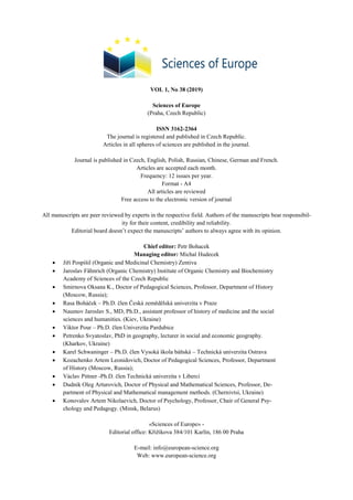
Сn =n*n= (1+n*Ho*c – n*H0. (4)
Analysis of the functional dependence of the ve-
locity leads to the establishment of a small deceleration
followed by a sharp peak by the deceleration of the pho-
ton associated with the decay into myriads MeeV Ω
(gravitons).
We come to the conclusion that the speed and the
loss of energy by photons are slowing down with each
pulsation, and then disintegrating into an array of grav-
itons!
2.3. Lifetime photons of course.
To define it, it suffices to specify in (3) the condi-
tion Сn ≡ 0, which leads
to such a connection the number of pulsations and
the initial wavelength of the photon, its the sort coordi-
0
50000
100000
150000
200000
250000
300000
350000
0 5 10 15 20 25 30 35 40
velositykm/s
distancy log n
Photon partial velocity km/s

17. Sciences of Europe # 38, (2019) 17
nates of the decay are c0/H0 = n*. And then calcu-
late the time photon life by the formula Tn = Dn/cn.
From the graphical dependence there is a parabola: Zc
= (n/nmax)/2, where nmax = a number of pul-
sations n = (eo – e)/Ω = ( where the depend-
ence on the initial photon energy eo (,555 nm) is dis-
covered. The current photon energy has a limit e ≤ er in
the field of relic photons! Analysis of the functional de-
pendence of the velocity leads to the establishment of a
small deceleration followed by a sharp peak by the de-
celeration
of the photon associated with the decay into myri-
ads MeeV Ω (gravitons).
We come to the conclusion that the speed and the
loss of energy by photons are slowing down with each
pulsation, and then disintegrating into an array of grav-
itons!
2.4. Dissolving ultra-cold radio waves in vac-
uum!
The radio waves include electromagnetic waves
with frequencies from 0.03 Hz to 3 THz, which corre-
sponds to a wavelength of 10 million km. up to 0.1 mm.
And the wavelength Ω is possible up to the boundary of
the Universe, and that is ~ 4.09E + 04 mpc! The ques-
tion is - what happens to the emission of photons of
long radio waves? From the analysis of the dependence
of the deceleration of photons on its energy Zc = [Ze/(1
+ Ze)]2
, the maximum value Zc ≤ 1 follows, and this is
possible at a speed c ≤, 5 * c from the initial one. And
then the photons are scattered on the elements of vac-
uum energy Ω with a wavelength to the size of the Uni-
verse! The speed of Ω varies from C to absorption by
thrones! The distribution of Ω over the velocities is
given by the offset - Zc = (n/nmax)2
, where nmax = eo/Ω
=  from the following considerations: at the time
of the photon’s decay, the energy elements Ω have
speed C and momentum p = Ω/c. And the spectrum of
radiation energy of primary photons, with a volumetric
explosion of quasars or galactic nuclei, determines the
superposition of the spectrum of already relic photons,
therefore the spectrum of pulses P (Ω) = Ω/C is also
equilibrium.
Why? And this is how the physical vacuum and
the structure of pulsating photons are arranged and re-
ally: Zc = (n/nmax)2
- this parabola sets the structure of
the star field and is essentially probabilistic in nature
because it generalizes huge arrays of experimental
facts! A decrease in the photon velocity is associated
with the loss of energy Ω with each pulsation!
2.5. Photon energy as a function of speed loss:
Using n = (eo–e)/Ω = (иnmax = eo/Ω =
 and nmax= eo/Ω =  we have as a result:
Zc = [Ze / (1 + Ze)]2
 (5)
Further, in connection with the establishment of a
finite lifetime of photons and a slowing down of their
propagation speed followed by their dissolution in a
vacuum environment, problems arise [1]! They had
been before, but they were not advertised, but simply
measured the displacement along the wavelength and
according to the Doppler effect, a road to nowhere! But
the changes in the energy or frequency of the radiation
somehow disfigured, well, they did not like to use it.
And the reason for this is that this feature is Z → 10
or more, but ≠  And then how to deal with the
identity Z≡ when Zc = 0, as required by the pos-
tulate of the constancy of the speed of light? The exist-
ence of the problem was also indicated by the fact that
the maxima of the equilibrium relict radiation curves
measured in the energy spectrum and the wavelengths
did not correspond — and this was indicated by Max
Planck! And as it turned out, there is a connection be-
tween the wavelength shifts and energy in this form:
Z = (1+(Ze/(1+Ze))2
)/(1+Ze) – 1. (6)
The main conclusion is that the inequality is al-
ways valid: Z>Ze and therefore Zс≠0! And the exper-
imental dependence of the thermodynamic temperature
of the background radiation on the wavelength is al-
most a straight line. The radiation spectrum of an abso-
lutely black body on such a graph seems to be straight,
parallel to the abscissa axis, and it turned out to meas-
ure the temperature of the CMB radiation. This fact
leads to the conclusion that there is an equilibrium
between the processes of natural increase in the con-
centration of relic photons and the processes of their
dissolution in vacuum.
§3. Resonances and Elementary Particles
-8
-7
-6
-5
-4
-3
-2
-1
0
1
32 33 34 35 36 37
LogZ
Log n - number of pulsation
Z - photon deceleration offset

18. 18 Sciences of Europe # 38, (2019)
3.1. Fundamental Law of the Defect of Communi-
cation Energy - DES.
The negation of the physical nature of a vacuum
had negative consequences for the physics of elemen-
tary particles. In the study of the -decay of the neu-
tron, n → p + e- + , it was found that the energy con-
servation law was violated by and Pauli put forward the
idea, in the absence of a vacuum environment, that this
energy is carried away by an unknown particle, the neu-
trino. And then with the discovery of new elementary
particles followed by the discovery of dozens of neu-
trino and antineutrino varieties, and naturally, with
such a mass of particles, no standard model, up to the
present time, is able to cope. And with the detection of
neutrinos, the great difficulties associated with the vir-
tually zero probability of its being captured by the at-
oms of the detectors, and the problem here is a misin-
terpretation of the process of violation of the energy
conservation law. As established [5], a neutrino is not a
particle, but a spherical G is a wave or a phantom, the
source of which is a deficit of binding energy (energy
elements) arising in the reactions of transformation of
elementary particles.
3.2. The hypothetically elusive neutrino parti-
cle is a phantom.
In the concept of the theory of thrones, problems
related to neutrinos are easily solved! The mass defect
is the binding energy and in transformation reactions it
is carried away with the emission of phantoms, which
have ultralow frequencies and, moreover, the pulsation
frequency during its capture, which occurs at the source
and target resonance during the transfer of n quanta
(garland) of radiant energy. And the process of energy
transfer takes place according to the pulsation tact, as
in the children's counting point “back and forth, you
and I are pleased,” and for the entire period between the
source and the detector, a connection has been estab-
lished with the Ariadne thread! And this connection can
neither be screened nor broken! And experiments with
a flat pendulum establish the existence of such electro-
magnetic radiation in the ultra-cold region in units of
hertz.
§4. What does the GRASS theory offer!
4.1. What did astronomers measure by displace-
ment ZH * r> 1 ... 10, from distant star objects?
Nothing valuable, because the partial speed of photons
slows down, which leads to a nonlinear increase in the
wavelength, as well as to energy loss, followed by dis-
solution in vacuum, to achieve its lifetime! And ignor-
ing the dissipative mechanism of energy loss by pho-
tons led to a misconception about the Universe with fic-
titious extensions, swelling and other attributes when
trying to explain the unfamiliar and save the postulate
of the constancy of the speed of light!
A feature was noted if we enter the intermediate
parameter n = (eo – e)/Ωthe number of pulsations, then
the main parameters, displacements and distances are
represented by linear functions n. And then, by (2, 3)
the nonlinear from n distance, group photon velocity,
and vacuum refractive index are calculated. For more
detailed analysis, you can use the functional depend-
ences Zc (Ze) and ZZe) given in (5.6).
4.2. As a consequence, the properties of the hy-
perspace [4] lead to the identity: Zt ≡ Zc, that is, the
uniform flow of world time is identical to the slow-
ing down of the speed of light. But the following state-
ment is also true: “the acceleration of deceleration of
the speed of light is identical to the slowing down of the
flow of world time”, which is the case for distant star
worlds this is when Z ≥1 and the equivalence of
Z≡ is violated! We conclude that when these con-
ditions are violated, the speed of light from distant stel-
lar objects slows down, which in turn slows down the
passage of time and increases the distance to them
[3,4]!
4.3. Equilibrium microwave radiation and relic
photons.
Suppose that a cavity with ideally reflecting walls
instead of a cube with an edge L has the shape of a
sphere with radius R. The reflecting walls fulfill the
boundary of the sphere with a stream of photons
through which it is outwards equal to the flow inward.
The dissipative process of photon energy loss Ω, for

19. Sciences of Europe # 38, (2019) 19
each pulsation, replenishes the process of multiple col-
lisions, and the mass model of the centers of birth of the
Universe provides a spherical isotropy of radiation. The
rest of the model of the equilibrium radiation of relic
photons according to Planck
Paradox. It is known that Planck proposed two
variants of the equilibrium radiation formula - for the
frequency scale and for the wavelength scale.
Amazingly, these two options, describing the spectrum
of the same radiation, give inconsistent positions of the
maximum of the spectral curve. If we compare these
two maxima on the scale of wavelengths, they differ
almost twice. Elementary logic suggests that both such
different positions of the maximum cannot be
confirmed by experiment. And, indeed, measurements
confirm only one version of Planck’s formula — for the
wavelength scale. Theorists prefer to work with the
frequency variant of the Planck formula, which
contradicts experience. But this paradox is solved
simply - to illustrate, we will use experimental data
from measurements of equilibrium microwave
radiation with maximum coordinates: wavelength
=1.9 mm and frequencies  = 160.4 GHz and
therefore, the partial speed of photons Cf = 304513.1
km/s And now an interesting question arises - why does
the partial velocity of photons in the region of the
maximum of the equilibrium radiation increase, while
the GRASS theory predicts its constant deceleration!
Without going into details of the conclusions of the
equilibrium radiation formulas, we note the following:
the formula for the energy spectrum has a complex non-
linear formula and therefore, even a small deviation
from the law C0 = 300000 km/s leads to a shift of
maxima, but not the fact that real partial speed Cp > c0!
§5. Phantom and the refractive index of vac-
uum!
5.1. Using the hyperspace interval in the form -
Sc = R ± i*c*t and the photon energy value - e = h* ±
i*(k), as well as the procedure for quantizing the dis-
tance by photons of electromagnetic radiation r = n *,
we find the value work on the transfer of quantum elec-
tromagnetic energy in the hyperspace of full dimension,
which leads to an invariant [1]:
An = (Sc*e) = n**(1+(с/с`= ))/2, (7)
where  is the refractive index of the vacuum
and if ≡ с/с`≈1 is the wave constant is the work of
moving the photon with the cost of Ω per pulsation!
Further, n is the quantum number of the distance,
but another interpretation is possible which determines
the state of the discrete package of electromagnetic ra-
diation, namely: for n = 1, equation (4) describes a
known quantum of energy - a photon; with n >> 2, 3 ...
N we have a more complex formation - a phantom, per-
haps a neutrino.
Experiments with a flat pendulum showed that
there are low-frequency emissions, but very high ener-
gies, which, in addition to the frequency (energy), also
have a pulsation frequency, and a propagation velocity
of electromagnetic radiation. Moreover, the ultra-low
frequency and long wavelength allows the phantom to
penetrate significant distances.
As an example: the observed collective or syn-
chronous radiation of many centers, which is recorded
at the birth of the alpha resonance effect of the planet
Earth and other solid-state planets of the solar system!
The impact is possible, both by processes in the planet
itself (earthquake), and by external causes - cataclysms
on the Sun or in outer space! The existence of such
states of phantoms, photon garlands, and predicts a
quantum equation for the work of An.
5.2. Solar neutrino history.
Neutrinos are, in fact, ultra cold photons and,
therefore, their lifetime is, of course, which is one of
the reasons for their elusiveness! Secondly, there are
problems in detecting ultra cold photons with high pen-
etrating power. For these reasons, solar neutrinos or de-
cay into an array of gravitons before reaching the Earth
or other planets (due to the neutrino energy discrete-
ness) and therefore skip the detectors! Actually, putting
Cn ≡ 0, we obtain the coordinates of the photon decay
and the relation from n → cn =
n*H0nn*H0
or:
R = n*= с0/H0
= 1,26281E+24 км =
4,09E+04 mpc. (8)
which leads to such a value of pulsations n =
1.21E+17*E (ev). On the other hand, the number of
pulsations n = n)/Ω and excluding n, we obtain
the value of the displacement of the energy of ultra cold
photons Ze = Ω*1.21E+17=1.89E-16, which is far be-
yond possibilities of measurement, but does not ex-
clude the probability of truth, provided that the photon
frequency is ≈ 160.4 GHz!
§6. The Rule of the Triad, Tron.
6.1. The triad cluster axiom: assuming the exist-
ence of both positively and negatively charged parti-
cles, there certainly exists a neutral particle of this clus-
ter. This rule holds for all clusters of elementary parti-
cles, with the exception of muon and electron.
Therefore, from the existence of an electron e-
, and a
positron e+
, it follows hypothetically the existence of a
very neutral particle of the throne - e0, which, for this
reason, has not been identified until now! And during
the annihilation reaction e+
+ e-
→ e0 (Tr) + 2, the
pseudo-neutralization of the elementary charges q + +
q- = Tr (e0) takes place. By the law of conservation of
elementary charges, they do not disappear, but are in a
bound state in the pulsation mode and this region is Tr!
And the energy state of the throne level determines a
quantum integer n of the number Ω [5]!
6.2. So there is a throne or Tr ≡ e0 → e-
+ e + 2*
To estimate the energy Tr, we use the approxima-
tion of the quantum harmonic oscillator: Em = ± (m +
½)*h*. ( throne oscillation frequency). From the
solution for the energy Em, it follows that the energy of
the quantum oscillator — the throne — has both a pos-
itive and a negative value and changes only in portions
and is quantized. Moreover, the positive energy is
bounded below by the minimum value E0 = ½*h*0 =
Ω - vacuum fluctuations, white noise, the energy of
zero-point oscillations is a direct consequence of the
uncertainty relation. This means that the throne energy
cannot be at the bottom of a potential well, but, in the
case of its negative value, there is no “bottom” of such